Abstract
In this paper, we propose a battery management algorithm to maximize the lifetime of a parallel-series connected battery pack with heterogeneous states of health in a battery energy storage system. The growth of retired lithium-ion batteries from electric vehicles increases the applications for battery energy storage systems, which typically group multiple individual batteries with heterogeneous states of health in parallel and series to achieve the required voltage and capacity. However, previous work has primarily focused on either parallel or series connections of batteries due to the complexity of managing diverse battery states, such as state of charge and state of health. To address the scheduling in parallel-series connections, we propose a cooperative multi-agent deep Q network framework that leverages multi-agent deep reinforcement learning to observe multiple states within the battery energy storage system and optimize the scheduling of cells and modules in a parallel-series connected battery pack. Our approach not only balances the states of health across the cells and modules but also enhances the overall lifetime of the battery pack. Through simulation, we demonstrate that our algorithm extends the battery pack’s lifetime by up to 16.27% compared to previous work and exhibits robustness in adapting to various power demand conditions.
1. Introduction
Lithium-ion batteries used in electric vehicles (EVs) have a finite lifetime, and for safety reasons must be replaced when their capacity drops to 80% or below [1]. However, these batteries can still be repurposed for other applications, where the remaining capacity is sufficient for less demanding tasks. Figure 1 illustrates the life cycle of lithium-ion batteries, where a battery energy storage system (BESS) can effectively utilize retired batteries when their state of health (SOH) is between 80% and 60% [2,3]. The BESS comprises one or more battery packs, each of which uses a group of battery cells connected in parallel and in series [4], to store electrical energy as backup power for households, data centers, charging stations, etc. [5]. Battery cells in a battery pack can be connected in one of two architectures shown in Figure 2: (a) a module groups the batteries in series, and then the modules are connected in parallel (denoted S-P), which is useful for high voltage applications; and (b) a module groups batteries in parallel, and then the modules are connected in series (denoted P-S) for applications requiring high capacity. In the past few years, many projects around the world have implemented a BESS by repurposing EV batteries. In the Netherlands, a 2.8 MWh BESS was installed for Johan Cruijff Arena in 2018 by reusing Nissan LEAF battery packs, each consisting of 192 cells, in an S-P connection [6]. In Finland, a 2.6 MWh BESS was built in 2021 as a backup power resource for the power grid by repurposing Tesla Model S battery packs, each consisting of 7104 cells, in a P-S connection [7]. Table 1 summarizes recent projects that repurposed EV batteries for a BESS. By leveraging a BESS, the demand for new batteries can be significantly reduced, thereby lessening the environmental impact associated with battery production. However, a BESS that reuses retired lithium-ion batteries from EVs still has some limitations when implemented.
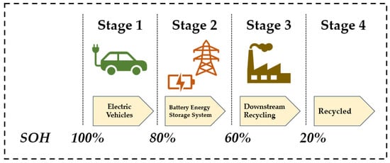
Figure 1.
Full life cycle of lithium-ion batteries.
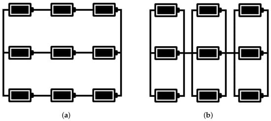
Figure 2.
Connections in a battery pack: (a) series-parallel (S-P), and (b) parallel-series (P-S).
One significant challenge in implementing a BESS is the varying capacity levels of the repurposed batteries connected in parallel and in series, indicating heterogeneous SOHs. The cells within a retired battery pack that exhibits heterogeneous SOHs can result in capacity and voltage imbalances, leading to inefficient energy storage and distribution [8]. This discrepancy in capacity can cause weaker cells to discharge faster or to overheat, potentially shortening the lifetime of the entire battery pack and posing safety risks. Furthermore, the varying SOHs among the cells complicates the task of maintaining balanced charging or discharging across the battery pack, making it difficult to achieve an optimal performance and lifetime [9]. As a result, the cells and modules need to be appropriately connected or bypassed (known as scheduling) to mitigate these issues and ensure the reliable operation of a BESS that reuses EV batteries.

Table 1.
Projects around the world that reused batteries from EVs.
Table 1.
Projects around the world that reused batteries from EVs.
| Name’s Project | Applications | Capacity | EV Model | Battery Pack Configuration |
|---|---|---|---|---|
| Johan Cruijff Arena (Netherlands) [6] | PV power supply, emergency supply | 2.8 MWh | 590 Nissan LEAF battery packs | 96S-2P 1 (192 cells) |
| Former coal-fired power plant in Elverlingsen (Germany) [7] | Energy storage system for households | 3.0 MWh | 72 Renault Zoe battery packs | 96S-2P (192 cells) |
| Cactos One Energy Storages (Finland) [10] | Energy storage system for households | 2.6 MWh | Tesla Model S battery packs | 74P-96S 2 (1704 cells) |
| EUREF Campus (Germany) [11] | Multi-use storage unit compensates for fluctuations in the grid | 1.9 MWh | Audi battery packs | 4P-108S (432 cells) |
| TGN Energy battery energy storage (Norway) [12] | Increased self-consumption | 216 kWh | Mercedes-Benz battery packs | NA |
| Landafors hydropower plant (Sweden) [13] | Offers fast frequency reserve regulation to the power markets | 250 kWh | 48 Volvo plug-in hybrid battery packs | NA |
1 Ninety-six series-connected batteries in a module, then two modules are connected in parallel. 2 Seventy-four parallel-connected batteries in a module, then 96 modules are connected in series.
In the BESS, switches are integrated to schedule cells and modules by connecting or bypassing them [14]. These switches enable scheduling to selectively isolate degraded cells or modules, thereby extending the battery pack’s useful lifetime [15]. By dynamically adjusting the connections between cells and modules, it is possible to balance the load effectively and mitigate the impact of lower capacity cells and modules. Scheduling not only improves the reliability and efficiency of the BESS, but also reduces the need for new batteries by maximizing the utilization of existing battery resources. To achieve this, scheduling requires all the states in the BESS including the state of charge (SOC) and the SOH of the cells and modules, the terminal voltage and output current of the battery pack, the power demand (e.g., from households), and the available power supply (e.g., from solar energy) [16,17,18]. The SOC of a battery indicates the current charge level as a percentage of its maximum capacity, whereas the SOH represents the ratio of the battery’s current maximum capacity to its original rated capacity. The required power demand and available power supply, collectively known as external systems information, refer to the amount of power the BESS needs to discharge and recharge. Incorporating BESS states into scheduling policy protects the battery pack by preventing excessive charging or discharging, and helps connect or bypass cells and modules appropriately. Furthermore, scheduling balances the SOC and SOH across cells and modules, ensuring that no single cell or module is overloaded [19]. In particular, SOH balancing through scheduling reduces the difference between SOHs among cells by utilizing the cells with higher SOHs and bypassing the cells with the lowest SOHs. In this way, the rate of degradation of cells or modules with lower SOHs is minimized. This balance helps to distribute the load more evenly, further protecting the battery pack and extending its useful lifetime.
Scheduling for battery packs in a BESS has been explored in the literature. In [20], an adaptive control algorithm was proposed to balance the SOCs for a series-connected battery pack. However, this approach overlooked the SOH and did not address parallel connections, limiting its effectiveness in comprehensive battery management. In [21], a controller was focused on balancing the SOCs in parallel-connected batteries to prevent overcharge or overdischarge, but failed to consider SOHs and series connections. An approach was presented in [15], where SOC balancing in parallel-series connections was proposed for automatic configuration according to the dynamic load, the storage demand, and the condition of each cell (i.e., SOC and current), yet it ignored SOH, which impacts a BESS lifetime. Other methods proposed in [18,22] were aimed at balancing SOHs by adjusting the charge and discharge durations for cells with weaker SOHs, but they ignored SOC and external systems information. Traditional methods like those presented in [15,18,20,21,22] are limited when they do not consider both SOC and SOH, because ignoring one can lead to suboptimal performance and reduced battery lifetime [19].
Deep reinforcement learning (DRL) has become a promising direction for battery pack scheduling with its ability to observe multiple states in a BESS and develop appropriate scheduling policies to optimize problem formulation. The combination of neural networks with reinforcement learning in DRL has proven to be a significant breakthrough, enabling the development of more scalable and efficient battery management strategies [23]. Unlike traditional reinforcement learning, which struggles with high-dimensional state spaces, DRL can leverage neural networks to approximate value functions and policies more effectively [24], allowing it to manage a larger number of cells and modules while responding in real time to critical factors such as SOC, SOH, and external systems information. In [17], an SOH balancing framework was proposed based on DRL in a series-connected battery pack to minimize the SOH imbalance among battery cells by observing the cell SOCs and SOHs. However, this approach lacked the observation of factors like power demand, terminal voltage, and output current, which are essential for effective switch scheduling and battery pack longevity. In [16], the authors proposed a DRL-based battery management algorithm to maximize the lifetime of retired batteries with varying SOHs in a parallel-connected battery pack, but they ignored scheduling for series-connected modules, so the approach was limited to applications requiring higher voltages. Moreover, the computational complexity in [16,17] was relatively high due to the extensive state space considered, and the proposals were limited to the use of a single agent, which can lead to a struggle with scalability when there is a large number of cells and modules. In [25], a multi-agent DRL-based method was proposed to reduce the SOC and SOH imbalance among battery cells, but overlooked external systems information, which directly affects battery pack lifetime by preventing overcharging or discharging, especially for cells or modules with lower SOHs. Table 2 shows the classification among battery scheduling algorithms.
Table 2.
Classification of battery scheduling algorithms.
In this study, we propose a battery management algorithm to maximize the BESS lifetime in a parallel-series connected battery pack with heterogeneous SOHs. To carry this out, the proposed algorithm first estimates the SOC and SOH of all cells jointly online. Then, based on the SOCs and SOHs of the cells and modules, a cooperative multi-agent deep Q network framework is implemented to schedule switches in the parallel-series connected battery pack by connecting or bypassing battery cells and modules. The proposed algorithm maximizes the battery pack lifetime and reduces the SOH imbalance among cells and modules. The algorithm also adapts to changes in external systems (i.e., power demand and available power supply). We demonstrate the effectiveness of our proposed algorithm via simulation using real, measured data compared to previous work.
The rest of this paper is organized as follows: Section 2 explores the proposed parallel-series connected battery pack and the associated scheduling challenges. Section 3 formulates the optimization problem by minimizing the reduction in SOH in the battery pack. Section 4 presents the framework of the proposed algorithm. Section 5 details the simulation setup, results, and the algorithm’s impact. Finally, Section 6 provides the conclusion of this work.
2. System Model
In this paper, we consider a parallel-series connected BESS [15] with a power supply (e.g., a solar energy generator) and a load (e.g., a household), as shown in Figure 3. The BESS comprises a parallel-series connected battery pack and a battery management system (BMS) that controls charging and discharging. We consider a discrete-time model with time slot t () and durations of .
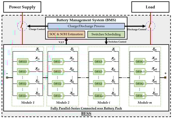
Figure 3.
An example of a parallel-series connected BESS.
2.1. Parallel-Series Connected Battery Pack Model
The battery pack consists of battery cells, where m battery modules are connected in series to increase voltage at the battery pack terminals, and n battery cells are connected in parallel to form a battery module to provide a higher current (or capacity), as shown in Figure 3. To schedule modules and cells in the battery pack, we consider controllable switches. Specifically, at time slot t, switch (, ) expresses connecting or disconnecting battery cell j of module i, denoted as cell , and switch is used to express connecting or bypassing module i in the battery pack. Switch for cell at time slot t is defined as
Switch for module i at time slot t is defined as
Switch is turned ON (1) if all n cells in module i are disconnected (0) to ensure that the battery pack charging or discharging process is not interrupted, which means module i is bypassed from the power supply or load at time slot t. Otherwise, switch is turned OFF (0) if any cell in module i is connected (1), which means that module i can be charged or discharged at time slot t.
Each battery cell is modeled according to a second-order Thévenin equivalent model [26] based on the material structure of the lithium-ion battery [25], as shown in Figure 4. Battery cell , which represents the jth cell in module i, has electrochemical impedance spectroscopy (EIS) parameters including open-circuit voltage , internal resistance , and two polarization RC pairs connected in series; each RC pair includes a resistor and a capacitor connected in parallel, i.e., (,) and (,). The terminal voltage of cell at time t, , is calculated by
where is the measured current of cell at time slot t; and , respectively, are the polarization voltages of RC pairs (,) and (,) in cell at time slot t, and are calculated by using the EIS parameters at the previous time slot as [26]
and
Based on measurement data (terminal voltage, current) and EIS parameters, the BMS estimates the SOC and SOH of each cell in order to schedule switches in the battery pack. Details are explained in the following subsection.
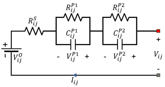
Figure 4.
Battery cell model.
2.2. Battery Management System
The BMS schedules the switches in the battery pack and external systems (i.e., the power supply or load demand) according to SOC and SOH estimation, as shown in Figure 3. To estimate SOC and SOH, the BMS monitors the voltage, current, and temperature of each battery cell. We define the SOC of cell at time t as the level of charge at time t relative to the maximum battery capacity by [18]
where is the estimated capacity level of cell at time slot t, and is the Coulombic efficiencies of the discharging and charging processes. We set the measured current to positive when discharged and negative when charged, to simplify Equation (6).
Module i, in which cells are connected in parallel, ensures that all cells share the same voltage while their individual currents add up, resulting in a cumulative increase in the total capacity of the module [27]. Therefore, capacity of module i in parallel connection is the sum of the capacities of the individual cells based on Kirchhoff’s law as [28]
We define the SOC of module i at time slot t as the ratio of the total charge level of all cells in module i to the total capacity of module i by [18]
The SOH of cell at time t, which is the ratio of the maximum battery capacity at time t to its rated capacity [29], is defined as
where is the initial capacity of new cell ; in this paper, we consider all battery cells to be the same type and have the same initial capacity as [30,31]. The BESS exhibits heterogeneous SOHs between individual cells. From Equation (7), capacity of module i at time slot t is the capacity summation of parallel-connected cells in the given module. Therefore, combining Equation (9), the SOH of module i at time slot t, , is defined as the SOH average of all parallel-connected cells in module i by
where is the SOH of cell j in module i at time slot t.
The SOH of individual aging cells is not uniform, leading to SOH inconsistencies between modules. The battery pack, in which modules are connected in series, decreases the terminal voltage, limiting the fulfillment of demand with lower SOH modules [32]. Therefore, we define the SOH of the battery pack, , as the lowest SOH of series-connected modules by [30,32]
where is the SOH of module i at time slot t. The SOH of the battery pack , which represents battery pack aging, is a non-increasing function until the end of its life cycle. In this paper, we define the lifetime of the battery pack, , as the first time slot after the battery pack reaches a threshold, denoted as , which is assumed to be 60% of SOH as seen in Figure 1, by
The BMS protects battery cells from overcharge, overdischarge, overheating, and excess current by controlling the BESS to fulfill demand when discharging to the load, then recharging from the power supply to recover power based on the SOC and SOH information. Note that the load and power supply change continuously under actual conditions, where and represent the power demand and available power supply, respectively, at time slot t and are constrained as [16]
which means the battery pack only charges, discharges, or is idle at the given time slot. We define the first time slot of a discharge process if and . Similarly, the first time slot of a charge process, , is defined if and . When discharging, the BMS considers the amount of discharged power, , and the maximum dischargeable power, , of the battery pack at time slot t as [33]
and
where indicates the lower bound of the SOC to prevent overdischarge, and is the first time slot of the discharge process containing t. When charging, the BMS considers the amount of charged power, , and the maximum chargeable power, , of the battery pack at time slot t as [33]
and
where indicates the upper bound of the SOC to prevent overcharging, and is the first time slot of the charge process containing t.
The BMS controls the battery pack discharge if and , or charge if and . Otherwise, the battery pack returns to idle for the remainder of the discharge or charge process. To that end, after estimating SOCs and SOHs, and controlling the charging or discharging process of the battery pack, the BMS schedules all switches in the battery pack in order to extend the lifetime and to reduce the SOH imbalance among the cells and modules.
3. Problem Formulation
The aim of this paper is to extend the lifetime of the battery pack in the BESS. To maximize the battery pack lifetime, we formulate the lifetime maximization of the battery pack as
where and represent the discharge current and charge current thresholds to limit the discharging and charging rates, respectively; and represent the lower and upper limits of the SOC, respectively, which are necessary to prevent overdischarging and overcharging; and represent the discharged and charged power, respectively, until time slot t; and , respectively, indicate the maximum power load of the battery pack when discharging and charging. Maximizing battery pack lifetime means maximizing the number of time slots in this second life cycle (Stage 2 in Figure 1). To carry this out, we minimize the rate of battery pack aging (i.e., the SOH reduction in the battery pack). We first define the SOH reduction in the battery pack at time slot t as
where and denote the SOH of the battery pack, respectively, at time slots and t. is a non-increasing function, so we constrain it with
To achieve this, the problem is framed to minimize the reduction in SOH of the battery pack, which is mathematically expressed as
4. The Proposed Algorithm
To enhance the lifetime of the battery pack in the BESS, we propose a battery management algorithm to minimize SOH reduction in the battery pack. The overall flow of the proposed algorithm is shown in Algorithm 1. At each time slot, the algorithm first gathers measurement data, including the terminal voltage, current, and temperature of each cell. It then estimates the SOC and SOH (Algorithm 2) and manages the BESS charging or discharging process based on the dynamic power demand (Algorithm 3). After updating the states in the BESS, the proposed algorithm schedules all switches in the battery pack to prolong its second lifetime based on the cooperative multi-agent deep Q network (Algorithm 4). The following subsections provide a detailed discussion of each component of the proposed algorithm.
| Algorithm 1 BESS Scheduling Algorithm |
|
| Algorithm 2 EKF-based SOC and SOH estimation |
|
| Algorithm 3 Charge, Discharge, and Idle Controlling |
|
| Algorithm 4 Switch Scheduling |
|
4.1. SOC and SOH Estimation
To observe the states of the battery pack, the proposed algorithm estimates the SOC and SOH of each battery cell by gathering its terminal voltage, current, and temperature. To carry this out, the algorithm first uses a fourth-order extended Kalman filter (EKF) to estimate the SOC and SOH of each battery cell, and then updates the SOC and SOH information of each battery module and the battery pack.
For each cell , we define the corrected state vector of cell at time , denoted as , by
Based on measured current and the modeled EIS parameters at the previous time slot, the algorithm estimates state vector and error covariance as
and
where is the correct state vector of cell at time ; and denote the transition matrix and the input matrix, respectively. Matrices and are defined as
and
where is the measured current of cell at . EIS parameters , , , , and are functions of and . Specifically, the EIS parameters are exponential functions of , such as
where , , and are real numbers, depending on the SOH of each cell . A dataset [34] is used to construct look-up tables of each EIS parameter , , , , or based on the above exponential functions. The algorithm estimates terminal voltage using state vector and Jacobian matrices and as
where is the measured current of cell at time slot t. Matrices and are, respectively, defined as
and
Open-circuit voltage is defined as the ath-order polynomial function of by
where is a real number depending on . The algorithm calculates Kalman gain to consider the error of the estimated value as
Using the measured terminal voltage of cell , , the algorithm corrects state vector and error covariance as
and
From corrected state vector , and maximum capacity of cell at time slot t are updated. The estimation algorithm updates the SOH of cell at time slot t by averaging it after completing a charge or a discharge process in the battery pack, as the SOH does not degrade immediately after single or multiple time slots [35], as
where and are the first time slots of the discharging and charging processes containing t. To that end, the estimation algorithm updates the SOC and SOH of modules () using Equations (8) and (10). of the battery pack is also updated using Equation (11). Algorithm 2 summarizes the EKF-based combined SOC and SOH estimation.
4.2. Charge, Discharge, and Idle Controlling
The proposed algorithm controls the charging and discharging processes of the battery pack to prevent overcharging and overdischarging in the BESS. By comparing loaded power (, and ), maximum power load (, and ), power demand (), and available power supply (), the algorithm determines whether the status of the BESS is discharging, charging, or idle in order to control it accordingly.
On the one hand, if the battery pack is discharging, i.e., , we calculate the amount of power discharged and maximum dischargeable power using Equations (14) and (15). If reaches power demand , the algorithm converts the BESS status from discharging to charging. When reaches the maximum power load of the battery pack when discharging , the algorithm lets the battery pack go idle. Otherwise, the discharge process continues.
On the other hand, if the battery pack is charging, i.e., , we calculate the amount of power charged and maximum chargeable power by using Equations (16) and (17). If reaches , the algorithm converts the BESS status from charging to discharging. When reaches the maximum power load of the battery pack at time slot t when charging , the algorithm lets the battery pack go idle. Otherwise, it continues charging. The process of the battery pack charging and discharging controlling is summarized in Algorithm 3.
4.3. Cooperative Multi-Agent Deep Reinforcement Learning-Based Battery Switch Scheduling
A cooperative multi-agent deep Q network (CM-DQN) scheduling algorithm is proposed to control switches in order to minimize the SOH reduction in the battery pack. The algorithm uses agents in which agent collectively evaluates the battery pack and comes up with module switch scheduling for serial connections, while m agents (1 to m) correspond to m modules for scheduling cell switches in parallel networks. While agents 1 to m optimize the local reward (i.e., minimize the SOH reduction in each module) by sharing policies, agent obtains global states (from modules and the BESS) to minimize the SOH reduction in the battery pack in the second life cycle. The proposed algorithm perceives environment state based on the estimation algorithm (Algorithm 2) and the charge and discharge control algorithm (Algorithm 3), and chooses a joint action by achieving a cumulative reward . The proposed switch scheduling algorithm first monitors the current environmental state of the battery pack and then derives state vectors for each agent, respectively, as
where and represent sets of the SOCs and SOHs of m series-connected modules, respectively; and are value sets of the SOCs and SOHs of n parallel-connected cells in module i, respectively; and represent the measured terminal voltage and the measured current of the battery pack at time slot t; and and are the load demand and available power supply at time slot t, respectively. Action with controls switches in the battery pack and is defined as
All agents continuously interact with each other by sharing states and policies so the training is synchronous and accurate.
To minimize SOH reduction in the battery pack in accordance with the obtained state, the algorithm utilizes acquired knowledge that includes a replay buffer to store in the form of with an experience in each time slot. For each agent , the algorithm constructs a main network , and a target network with the same structure and random weights , where approximates the action-value function at time slot t, and computes the target action value .
To utilize the past experiences, the proposed algorithm looks at acquired knowledge to determine whether state is in or not. If state belongs to , the algorithm chooses action using an -greedy policy [36]. Specifically, it either chooses a random action with probability or opts for the action with the highest with probability , by
In the case in which state is not in , scheduling action is performed at random. We determine which modules are bypassed at time slot t, and then limit scheduling action in each agent of cell switch scheduling (agent 1 to m). If module i is bypassed, we limit action by turning OFF all cells in module i. Otherwise, the algorithm continues to assess the acquired knowledge to determine whether state is included in . If state is in , the algorithm selects action according to an -greedy policy as specified in Equation (38). In the case in which state is not in , scheduling action is chosen randomly. After all actions are chosen, a joint action is executed.
For agent i of module i corresponding to cell switch scheduling, the algorithm evaluates the local immediate reward as
where is the SOH reduction in module i at time slot t, and is defined as a non-increasing function by
The algorithm evaluates the local cumulative reward through interactions with the environment and seeks an optimal policy to maximize it as
To that end, the algorithm computes the global cumulative reward to minimize SOH reduction in the battery pack as
where is the global immediate reward and is computed by
By executing joint action , the algorithm updates new state , then stores sample into accquired knowledge . Target action value is computed by
where is the discount factor that determines the emphasis on future rewards. The CM-DQN updates the acquired knowledge by minimizing the loss function through gradient descent. The loss function is defined as
Weight is updated by the loss function as
where is the learning factor. After computing the loss for an action, the target network updates its weights to match those of the main network , i.e., after P time slots to ensure algorithm stability [36]. Loss function is minimized so that action value has the same value as target action value , which also means that the SOH reduction in the battery pack is minimized. The proposed switch scheduling algorithm is summarized in Algorithm 4. The training process in the CM-DQN is shown in Figure 5.
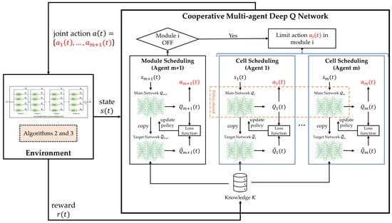
Figure 5.
The training process in the cooperative multi-agent deep Q network.
5. Performance Evaluation
5.1. Simulation Environment
The BESS was performed via simulation using a lithium-ion battery pack model and was implemented in MATLAB and Simulink 2023b. To assess the performance of the proposed algorithm, we designed a parallel-series connected battery pack [15], listed in Table 3, including 24 lithium-ion batteries with heterogeneous SOHs. The battery cell was modeled as a second-order Thévenin equivalent battery model with reductions in SOHs by utilizing a NASA dataset [34]. That dataset includes 28 lithium-ion cobalt oxide 18,650 cells with a nominal voltage of 3.7 V and nominal capacity of 2.2 Ah with a maximum current of 4 A, encompassing real-time measurements of terminal voltage, current, cell temperature, discharging capacity, and EIS impedance readings. We identified the EIS parameters, including , , , , , and , in the 90% to 60% SOH range by using the dataset. A dynamic power demand condition was used to evaluate the effectiveness of the algorithm. The power demand was obtained by generating values from a uniform distribution within 60 Wh to 100 Wh, while the terminal voltage was obtained by generating values from a uniform distribution ranging from 13.75 V to 16.25 V (at least four series-connected modules ON at a given time because the nominal voltage of each cell is 3.7 V). We set the load current for both discharging and charging the battery pack to 8 A (at least two parallel-connected batteries ON at a given time because the maximum output current of one battery is 4 A).
Table 3.
Initial SOHs of the cells and modules.
Two deep Q network architectures were constructed for cell scheduling and module scheduling, each including one input layer, two hidden layers, and one output layer. The number of hidden layers and the number of neurons in each hidden layer can be selected by trial and error [37]. To determine the optimal network size, including the number of hidden layers and the number of neurons in each layer, two approaches are commonly used: the constructive approach and the destructive approach [38]. We used a constructive approach to network sizing [39]. We started with a small network and gradually added neurons or hidden layers to improve the performance of the network, where the number of hidden layer neurons varied among 64, 128, and 256, and the number of hidden layers started from 1. Both deep Q network architectures with two 128-dimension hidden layers had the maximum cumulative reward with minimum episodes. For cell scheduling, the input layer included 11 neurons corresponding to the number of dimensions in state of module i with four parallel-connected cells. The output layer consisted of 12 neurons corresponding to possible actions, , for cell switch scheduling. For module scheduling, the input layer included 15 neurons corresponding to the number of dimensions in state of the battery pack with six series-connected modules. The output layer consisted of 15 neurons corresponding to possible actions, , for module switch scheduling. During learning, we set the learning rate to 0.001, which helped reduce the loss function episodes and balance the speed of learning with the stability of the training process. We set the discount factor to 0.99 to effectively balance prioritizing long-term cumulative rewards, i.e., minimizing SOH reduction in the battery pack, while avoiding slowing down the convergence process. Other simulation parameters are summarized in Table 4.
Table 4.
Simulation parameters.
For the performance evaluation, we first investigated the effect of the proposed algorithm on SOH balancing to enhance the lifetime of the battery pack. Then, we evaluated the impact of the proposed algorithm on dynamic power demand. To validate the performance of the proposed cooperative multi-agent deep Q network (denoted as CM-DQN) algorithm, we compare it with previous works, including a self-X multicell battery algorithm [15] denoted as Self-X, a multilayer SOH equalizer [22] denoted as M-SOH, a DOD-SOH balancing algorithm [17] denoted as DOD-SOH, and a multi-actor–critic scheduling algorithm [25] denoted as M-A2C.
5.2. Capacity Balancing and Battery Pack Lifetime
We evaluated the performance of the proposed algorithm on balancing the SOH of modules, as shown in Figure 6. The SOH balancing of modules in the battery pack in all the algorithms is shown in Figure 6a–e. The proposed algorithm (CM-DQN) achieved more SOH balancing than previous work. During learning, the CM-DQN framework determines the optimal actions known as switches to connect or bypass cells and modules by observing BESS states such as the SOCs and SOHs of cells and modules, power demand , or available power supply . CM-DQN ensures that no single module degrades significantly faster than the others by fully observing the states in the BESS (including SOC, SOH of modules and cells, charging and discharging states, and the power demand). Figure 6f compares the standard deviation in SOHs among the modules over time for each algorithm. CM-DQN exhibited the lowest standard deviation (close to zero), compared to previous work, further affirming its ability to maintain SOH balance among modules. Self-X showed an SOH imbalance that was almost unchanged without considering SOHs. Other methods (M-SOH, DOD-SOH, and M-A2C), which considered SOHs, reduced the SOH imbalance but, without observations of the states in the BESS, the standard deviation was still higher than CM-DQN, indicating that SOHs between modules were not balanced until the end of the lifetime. With heterogeneous SOHs in the battery pack, CM-DQN offered better performance than other algorithms by balancing SOHs among the modules.
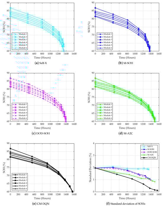
Figure 6.
SOH balancing with different methods.
The performance of the proposed algorithm on battery pack lifetime, measured by minimizing SOH reduction, was evaluated and is shown in Figure 7. By balancing the SOHs among the modules in the battery pack, the proposed algorithm (CM-DQN) achieved the lowest SOH reduction in the battery pack compared to the other algorithms by minimizing the SOH reduction for each time slot, as shown in Figure 7a. The reduction in SOH under Self-X and M-SOH increased rapidly after 1200 h, compared to the other algorithms, due to the lack of consideration of both SOC and SOH. M-A2C had the closest performance to CM-DQN, but ignoring external systems information caused the SOH reduction, , to increase faster as the battery lifetime weakened after 1250 h. The SOH reduction in the battery pack was minimized with CM-DQN, resulting in an extended battery pack lifetime, as shown in Figure 7b. The proposed algorithm CM-DQN achieved a longer battery pack lifetime compared to previous work. The SOH of the battery pack under CM-DQN reached 60% (the end of its second life) after a working time of 1558 h. By not observing the states in the BESS, all other work finished the second lifetimes significantly faster than CM-DQN. Table 5 shows that the battery pack lifetime improvement of the proposed algorithm (CM-DQN) compared to previous work was up to 16.27%. Hence, the proposed algorithm can efficiently schedule switches in the battery pack to maximize the BESS lifetime and balance the SOHs among the modules and cells.
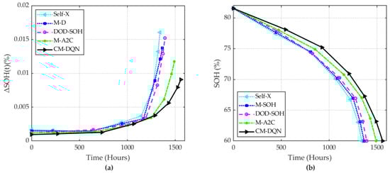
Figure 7.
Extending lifetime of the battery pack with (a) SOH reduction per time slot, and (b) maximum lifetime of the battery pack until reaching 60% of SOH.
Table 5.
Battery pack lifetime improvement of the proposed algorithm compared with previous work.
To show the impact of SOC balancing on the lifetime of the battery pack, the standard deviations of the SOCs in a battery pack under different algorithms are shown in Figure 8. Self-X, which only focused on SOCs, had better SOC balancing than other algorithms but stopped decreasing after some time and had a worse battery pack lifetime, as shown in Figure 7b. CM-DQN had a continuously decreasing standard deviation over time and it was lower than that of Self-X after 1130 h. Although the proposed algorithm (CM-DQN) focused on only balancing the SOHs of cells by observing SOCs, it also decreased the SOC imbalance among the cells in a battery pack and achieved a longer lifetime. As a result, scheduling cells and modules in a battery pack for SOH balancing is more important to extend the lifetime of the battery pack, as shown in Figure 6f, Figure 7 and Figure 8.
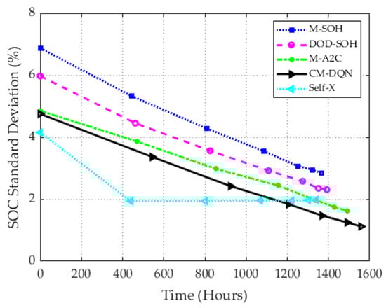
Figure 8.
Standard deviation of SOCs among modules.
5.3. Performance of the Proposed Algorithm on Varied Demands
We studied the performance of the proposed algorithm in scenarios with different power demands, as shown in Table 6. We considered various conditions in Scenario 1 with the same mean (80 Wh) and incremental variance (from 8.33 to 533.33), as shown in Figure 9a, and in Scenario 2 with the same variance (133.33) and incremental mean (from 60 Wh to 100 Wh), as shown in Figure 9b. Understanding the impact of demand variance is essential for evaluating the robustness and adaptability of battery management algorithms in real-world applications.
Table 6.
Different energy demand conditions.
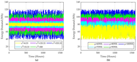
Figure 9.
Energy demand profiles with (a) Scenario 1, and (b) Scenario 2.
Figure 10 illustrates the impact of different load demand conditions, characterized by varying demand variance (), on the lifetime of algorithms under the same mean demand. In Figure 10a, it is observed that, as the demand variance increased from 8.33 to 533.33, the standard deviation for all algorithms also increased. The proposed algorithm minimizes the SOH reduction in the battery pack at each time slot by balancing the SOHs of the battery modules. The charge and discharge control algorithm (Algorithm 3) and observation of dynamic demands (shown in state vectors in (36)) helped CM-DQN consistently achieve the lowest standard deviation, indicating robustness against fluctuations in demand. In contrast, the previous algorithms showed an increasing standard deviation proportional to the variation in power demand, indicating a lack of adaptation to demand dynamics. Figure 10b examines the lifetime obtained by the algorithms. The proposed algorithm (CM-DQN) demonstrated a significantly longer lifetime than the others, maintaining a robust performance in SOH balancing and extending lifetime even as demand variance increased. This suggests the proposed algorithm is more adaptive and effective in extending a battery’s operational lifetime under varying demand conditions. In summary, the proposed CM-DQN algorithm outperformed the others in robustness (lower standard deviation and longer lifetime) when subjected to increasing demand variance.
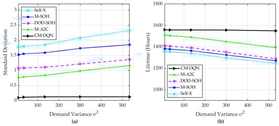
Figure 10.
Performance of the scheduling algorithms under dynamic power demand in Scenario 1: (a) standard deviations in SOHs among the modules and (b) operation times of the battery pack until the SOH reached 60%.
Figure 11 presents the performance of the algorithms under different mean demand conditions () while keeping the variance constant. Figure 11a shows the standard deviation of the algorithms’ performance as the demand mean increased from 60 Wh to 100 Wh. The CM-DQN algorithm consistently achieved the lowest standard deviation, indicating its robustness against variations in the demand mean. Figure 11b illustrates the lifetimes of the algorithms as the demand mean increased. The proposed CM-DQN algorithm exhibited the longest lifetime across all mean demand levels, demonstrating its efficiency in extending the battery lifetime under varying power demands. Overall, CM-DQN minimized the SOH reduction in the battery pack in handling different demand mean conditions, providing an extended battery lifetime and an SOH balancing among the modules.
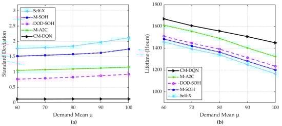
Figure 11.
Performance of the scheduling algorithms under dynamic power demand in Scenario 2: (a) standard deviation in SOHs among the modules and (b) operation time of the battery pack until the SOH reached 60%.
6. Conclusions
In this paper, we proposed a battery management algorithm using a cooperative multi-agent deep Q network to maximize battery lifetimes for the battery pack in a BESS. The BESS consisted of a battery pack in which retired batteries with heterogeneous SOHs are connected in parallel and series. The proposed algorithm scheduled switches in the battery pack by connecting or bypassing battery cells and modules. The algorithm maximized the battery pack lifetime by reducing the SOH imbalance among cells and adapting to varied power demands. Via simulation, we showed that the proposed algorithm outperformed the other algorithms by attaining a more extended battery pack lifetime and reduced SOH imbalance among the cells and modules. The proposed algorithm extended the lifetime of the battery pack by up to 16.27% compared to the other algorithms.
Author Contributions
Conceptualization, N.Q.D., S.M.S. and S.K.; methodology, N.Q.D., S.M.S., S.-J.C. and S.K.; software, N.Q.D.; validation, S.M.S., T.M.D., S.-J.C. and S.K.; formal analysis, N.Q.D., S.M.S., T.M.D. and S.K.; investigation, N.Q.D., S.M.S., T.M.D. and S.K.; writing—original draft preparation, N.Q.D., S.M.S. and T.M.D.; supervision, S.K. All authors have read and agreed to the published version of the manuscript.
Funding
This work was supported by the Basic Science Research Program through the National Research Foundation of Korea (NRF), funded by the Ministry of Education (NRF-2021R1I1A3A04037415) and the Korea Hydro and Nuclear Power Co. (2023).
Data Availability Statement
Publicly available datasets were analyzed in this study. These data can be found here: https://www.nasa.gov/intelligent-systems-division/discovery-and-systems-health/pcoe/pcoe-data-set-repository/ (accessed on 22 July 2024).
Conflicts of Interest
The funding sponsors had no role in the design of the study; in the collection, analyses, or interpretation of data; in the writing of the manuscript, or in the decision to publish the results.
References
- Hunt, G. USABC Electric Vehicle Battery Test Procedures Manual; Revision 2; United States Department of Energy: Washington, DC, USA, 1996.
- Examples for Reuse of Power Batteries. In Reuse and Recycling of Lithium-Ion Power Batteries; John Wiley & Sons, Ltd.: Hoboken, NJ, USA, 2017; Chapter 3; pp. 261–334.
- Canals Casals, L.; García, B.; Aguesse, F.; Iturrondobeitia, A. Second life of electric vehicle batteries: Relation between materials degradation and environmental impact. Int. J. Life Cycle Assess. 2015, 22, 82–93. [Google Scholar] [CrossRef]
- Wang, L.; Yusheng, S.; Wang, X.; Wang, Z.; Zhao, X. Reliability Modeling Method for Lithium-ion Battery Packs Considering the Dependency of Cell Degradations Based on a Regression Model and Copulas. Materials 2019, 12, 1054. [Google Scholar] [CrossRef] [PubMed]
- Martinez-Laserna, E.; Gandiaga, I.; Sarasketa-Zabala, E.; Badeda, J.; Stroe, D.I.; Swierczynski, M.; Goikoetxea, A. Battery second life: Hype, hope or reality? A critical review of the state of the art. Renew. Sustain. Energy Rev. 2018, 93, 701–718. [Google Scholar] [CrossRef]
- Europe’s Largest Energy Storage System Now Live at the Johan Cruijff Arena. Available online: https://global.nissannews.com/en/releases/europes-largest-energy-storage-system-now-live-at-the-johan-cruijff-arena/ (accessed on 22 July 2024).
- Second Life for a Coal Power Plant in Germany. Available online: https://www.electrive.com/2020/11/24/second-life-for-a-coal-power-plant-in-germany/ (accessed on 22 July 2024).
- Nováková, K.; Pražanová, A.; Stroe, D.I.; Knap, V. Second-Life of Lithium-Ion Batteries from Electric Vehicles: Concept, Aging, Testing, and Applications. Energies 2023, 16, 2345. [Google Scholar] [CrossRef]
- Rouholamini, M.; Wang, C.; Nehrir, H.; Hu, X.; Hu, Z.; Aki, H.; Zhao, B.; Miao, Z.; Strunz, K. A Review of Modeling, Management, and Applications of Grid-Connected Li-Ion Battery Storage Systems. IEEE Trans. Smart Grid 2022, 13, 4505–4524. [Google Scholar] [CrossRef]
- Cactos One Energy Storages. Available online: https://www.cactos.fi/en/product/ (accessed on 22 July 2024).
- Audi Opens Battery Storage Unit on Berlin EUREF Campus. Available online: https://www.mobilityhouse.com/media/productattachments/files/en20190524_Audi_opens_battery_storage_unit.pdf (accessed on 22 July 2024).
- A. Market-Intelligence-Report-December-2022. Available online: https://projectcobra.eu/wp-content/uploads/2022/12/Market-Intelligence-Report-December-2022.pdf (accessed on 22 July 2024).
- Fortum Installs Innovative Battery Solution at Landafors Hydropower Plant in Sweden. Available online: https://www.fortum.com/media/2021/04/fortum-installs-innovative-battery-solution-landafors-hydropower-plant-sweden (accessed on 22 July 2024).
- Why CellSwitch™ Is Revolutionary for Batteries. Available online: https://www.relectrify.com/technology/cellswitch/ (accessed on 22 July 2024).
- Kim, T.; Qiao, W.; Qu, L. Power Electronics-Enabled Self-X Multicell Batteries: A Design toward Smart Batteries. IEEE Trans. Power Electron. 2012, 27, 4723–4733. [Google Scholar]
- Doan, N.Q.; Shahid, S.M.; Choi, S.J.; Kwon, S. Deep Reinforcement Learning-Based Battery Management Algorithm for Retired Electric Vehicle Batteries with a Heterogeneous State of Health in BESSs. Energies 2024, 17, 79. [Google Scholar] [CrossRef]
- Yang, X.; Liu, P.; Liu, F.; Liu, Z.; Wang, D.; Zhu, J.; Wei, T. A DOD-SOH balancing control method for dynamic reconfigurable battery systems based on DQN algorithm. Front. Energy Res. 2023, 11, 1333147. [Google Scholar] [CrossRef]
- Ma, Z.; Gao, F.; Gu, X.; Li, N.; Wu, Q.; Wang, X.; Wang, X. Multilayer SOH Equalization Scheme for MMC Battery Energy Storage System. IEEE Trans. Power Electron. 2020, 35, 13514–13527. [Google Scholar] [CrossRef]
- Shen, L.; Li, J.; Meng, L.; Zhu, L.; Shen, H.T. Transfer Learning-Based State of Charge and State of Health Estimation for Li-Ion Batteries: A Review. IEEE Trans. Transp. Electrif. 2024, 10, 1465–1481. [Google Scholar] [CrossRef]
- Chowdhury, S.; Shaheed, M.N.B.; Sozer, Y. State-of-Charge Balancing Control for Modular Battery System with Output DC Bus Regulation. IEEE Trans. Transp. Electrif. 2021, 7, 2181–2193. [Google Scholar] [CrossRef]
- Abdalla, A.A.; Moursi, M.S.E.; El-Fouly, T.H.M.; Hosani, K.H.A. Reliant Monotonic Charging Controllers for Parallel-Connected Battery Storage Units to Reduce PV Power Ramp Rate and Battery Aging. IEEE Trans. Smart Grid 2023, 14, 4424–4438. [Google Scholar] [CrossRef]
- Li, N.; Gao, F.; Hao, T.; Ma, Z.; Zhang, C. SOH Balancing Control Method for the MMC Battery Energy Storage System. IEEE Trans. Ind. Electron. 2018, 65, 6581–6591. [Google Scholar] [CrossRef]
- Wang, X.; Wang, S.; Liang, X.; Zhao, D.; Huang, J.; Xu, X.; Dai, B.; Miao, Q. Deep Reinforcement Learning: A Survey. IEEE Trans. Neural Networks Learn. Syst. 2024, 35, 5064–5078. [Google Scholar] [CrossRef] [PubMed]
- Wu, L.; Lyu, Z.; Huang, Z.; Zhang, C.; Wei, C. Physics-based battery SOC estimation methods: Recent advances and future perspectives. J. Energy Chem. 2024, 89, 27–40. [Google Scholar] [CrossRef]
- Sui, Y.; Song, S. A Multi-Agent Reinforcement Learning Framework for Lithium-ion Battery Scheduling Problems. Energies 2020, 13, 1982. [Google Scholar] [CrossRef]
- Hu, X.; Li, S.; Peng, H. A comparative study of equivalent circuit models for Li-ion batteries. J. Power Sources 2012, 198, 359–367. [Google Scholar] [CrossRef]
- BU-302: Series and Parallel Battery Configurations. Available online: https://batteryuniversity.com/article/bu-302-series-and-parallel-battery-configurations# (accessed on 22 July 2024).
- von Bülow, F.; Meisen, T. A review on methods for state of health forecasting of lithium-ion batteries applicable in real-world operational conditions. J. Energy Storage 2023, 57, 105978. [Google Scholar] [CrossRef]
- Lipu, M.H.; Hannan, M.; Hussain, A.; Hoque, M.; Ker, P.J.; Saad, M.; Ayob, A. A review of state of health and remaining useful life estimation methods for lithium-ion battery in electric vehicles: Challenges and recommendations. J. Clean. Prod. 2018, 205, 115–133. [Google Scholar] [CrossRef]
- Hua, Y.; Cordoba-Arenas, A.; Warner, N.; Rizzoni, G. A multi time-scale state-of-charge and state-of-health estimation framework using nonlinear predictive filter for lithium-ion battery pack with passive balance control. J. Power Sources 2015, 280, 293–312. [Google Scholar] [CrossRef]
- Chang, C.Y.; Tulpule, P.; Rizzoni, G.; Zhang, W.; Du, X. A probabilistic approach for prognosis of battery pack aging. J. Power Sources 2017, 347, 57–68. [Google Scholar] [CrossRef]
- Jeng, S.L.; Tan, C.M.; Chen, P.C. Statistical distribution of Lithium-ion batteries useful life and its application for battery pack reliability. J. Energy Storage 2022, 51, 104399. [Google Scholar] [CrossRef]
- Lucaferri, V.; Quercio, M.; Laudani, A.; Riganti Fulginei, F. A Review on Battery Model-Based and Data-Driven Methods for Battery Management Systems. Energies 2023, 16, 7807. [Google Scholar] [CrossRef]
- Bole, B.; Kulkarni, C.; Daigle, M. Randomized Battery Usage Data Set. In NASA Prognostics Data Repository; NASA Ames Research Center: Moffett Field, CA, USA, 2009. [Google Scholar]
- Liu, X.; Li, J.; Yao, Z.; Wang, Z.; Si, R.; Diao, Y. Research on battery SOH estimation algorithm of energy storage frequency modulation system. Energy Rep. 2022, 8, 217–223. [Google Scholar] [CrossRef]
- Sutton, R.S.; Barto, A.G. Reinforcement Learning: An Introduction; A Bradford Book: Cambridge, MA, USA, 2018. [Google Scholar]
- Basheer, I.; Hajmeer, M. Artificial neural networks: Fundamentals, computing, design, and application. J. Microbiol. Methods 2000, 43, 3–31. [Google Scholar] [CrossRef]
- Alpaydin, E. Introduction to Machine Learning; MIT Press: Cambridge, MA, USA, 2020. [Google Scholar]
- Shahid, S.M.; Ko, S.; Kwon, S. Real-Time Classification of Diesel Marine Engine Loads Using Machine Learning. Sensors 2019, 19, 3172. [Google Scholar] [CrossRef]
Disclaimer/Publisher’s Note: The statements, opinions and data contained in all publications are solely those of the individual author(s) and contributor(s) and not of MDPI and/or the editor(s). MDPI and/or the editor(s) disclaim responsibility for any injury to people or property resulting from any ideas, methods, instructions or products referred to in the content. |
© 2024 by the authors. Licensee MDPI, Basel, Switzerland. This article is an open access article distributed under the terms and conditions of the Creative Commons Attribution (CC BY) license (https://creativecommons.org/licenses/by/4.0/).