Research on Optimal Scheduling Strategy of Differentiated Resource Microgrid with Carbon Trading Mechanism Considering Uncertainty of Wind Power and Photovoltaic

Abstract

Accelerating the green transformation of the power system is the inevitable path of the energy revolution; the increasing installed capacity of new energy and the penetration rate of electricity, uncertainty regarding new energy output, and the rising proportion of distributed power supply access have led to the threat against the safe and stable operation of the current power system. With the increasing uncertainty on both sides of power supply and demand, the microgrid (MG) is needed to effectually aggregate, coordinate, and optimize resources, such as adjustable resources, distributed power supply, and distributed energy storage in a certain area on the demand side. Therefore, in this paper, the uncertainty of wind power and PV is first dealt with by Latin hypercube sampling (LHS). Secondly, differentiated resources in the MG region can be divided into adjustable resources, distributed power supply, and energy storage. Adjustable resources are classified according to demand response characteristics. At the same time, the MG operating cost and carbon trading mechanism (CTM) are comprehensively considered. Finally, a low-carbon economy optimal scheduling strategy with the lowest total cost as the optimization goal is formed. Then, in order to verify the effectiveness of the proposed algorithm, three different scenarios are established for comparison. The total operating cost of the proposed algorithm is reduced by about 30%, and the total amount of carbon trading in 24 h can reach nearly 600 kg, bringing economic and social benefits to the MG.

1. Introduction

As the climate issue has gradually become a global consensus and countries have taken measures to control carbon emissions, a large number of new energy units represented by wind and solar energy have emerged in the new power system. However, the volatility of wind and solar power output weakens the stability foundation of the grid system and increases the imbalance of the power system, making it impossible to ensure the consumption of new energy while taking into account reliability and economy [1,2,3,4].

Microgrid (MG) optimal dispatch is one of the crucial methods to achieve efficient utilization and local consumption of distributed generation (DG) sources, including renewable energy units [5]. It optimizes the allocation of distributed resources, such as wind power and photovoltaic systems, intelligently adjusts the balance between supply and demand, and increases the proportion of renewable energy output, thereby reducing the economic costs of the microgrid. Most renewable energy units rely on weather-sensitive sources, like wind and solar energy, for power generation, resulting in complex and variable scenarios with significant intra-period fluctuations and making accurate forecasting and dispatching challenging. Additionally, the primary focus is often on economic benefits, with limited attention given to green indicators such as carbon emissions, which hinders the achievement of “green, low-carbon and economical” goals. The introduction of a carbon emissions trading market mechanism can address this issue.

Currently, scholars both domestically and internationally have conducted extensive research on microgrid optimal dispatch strategies. In the realm of microgrid optimal dispatch research, improvements to the particle swarm optimization (PSO) algorithm are frequently employed to tackle nonlinear multi-objective optimization problems. For instance, reference [6] proposes an optimization method based on the multi-agent chaotic particle swarm optimization (MACPSO) algorithm for large-scale electric vehicles participating in microgrid operation management, which mitigates the impact of microgrids on the main grid and enhances overall economic efficiency. In [7], the authors introduce an improved multi-objective particle swarm optimization (MOPSO) algorithm by incorporating linearly decreasing differential weights and mutation strategies, achieving cost reduction and efficiency enhancement in microgrid operation. In [8], the authors construct a day-ahead and intra-day coordinated optimal dispatch model for microgrids using a data-driven multi-discrete scenario robust approach, ensuring safe and economical microgrid operation. In [9], the authors employ phasor particle swarm optimization (PPSO) to solve the optimal dispatch problem of microgrids incorporating renewable energy sources. Additionally, with technological advancements, new-generation technologies, such as deep reinforcement learning (DRL) [10], have also entered the field of microgrid optimal dispatch. In [11], the authors suggest applying DRL algorithms to power grids with distributed flexible resources, demonstrating good scalability and transferability and thereby enhancing the overall performance of microgrids. However, most of these studies focus on relatively simple scenarios and fail to consider the “double-high” characteristics of today’s distribution systems, namely “high proportions of renewable energy sources such as wind and solar power” and “high proportions of power electronic devices”. This makes it difficult to address the uncertainties in optimization dispatch strategies caused by the volatility of renewable energy sources, like wind and solar power. While optimization algorithms such as particle swarm optimization (PSO) can achieve good results for large datasets, for some small microgrids, the excessive complexity of the models can lead to issues like long computation times and overfitting.

In addressing the uncertainty of wind and solar power, many scholars have researched wind and photovoltaic forecasting algorithms, incorporating numerous weather features to ensure the validity of the output curves. However, in many regions of microgrid operations, only a small number of renewable energy generation devices exist, and it suffices to ensure the output’s effectiveness within a certain error range, with other generation devices compensating for the electricity load demand. For instance, reference [12] addresses the uncertainty of wind and solar output by combining Monte Carlo sampling to simulate wind and solar output scenarios, then utilizing scenario reduction techniques to obtain the most probable wind and solar output data of a typical scenario. In comparison with the wind and solar output results from this reference, the algorithm presented in this paper demonstrates superior advantages. Reference [13] proposes a hybrid energy storage allocation strategy based on empirical mode decomposition (EMD) technology and a two-stage robust approach, reducing wind power fluctuations and enhancing the energy efficiency and sustainability of data centers. Reference [14] introduces an improved dynamic group cooperation optimization algorithm to predict the output of wind–solar hybrid power stations. While these methods address the uncertainty of wind and solar output, they not only increase model complexity but also fail to consider the economic costs and carbon emission levels of operating equipment. Therefore, integration with emerging mechanisms, such as carbon emissions trading markets, can effectively balance economic and environmental concerns.

In the study of carbon trading markets, reference [15] proposes a stepped carbon trading mechanism that enhances the emissions reduction incentives of power supply systems compared to traditional carbon trading mechanisms. Reference [16] introduces a rolling settlement mechanism for the electricity–carbon joint market, which considers the unit load rate–carbon emissions intensity curve and a centralized carbon trading mechanism. This mechanism aims to maximize the benefits of both carbon pricing and the joint market while saving time costs.

Based on this background, this paper intends to solve the problem, and its main contributions are as follows: (1) In order to solve the uncertainty of the wind landscape output, the Latin hypercube sampling method is adopted in this paper, as it is more effective in removing the uncertainty problem than the popular Monte Carlo method [17]. (2) The carbon trading market, which is vigorously developed at present, has to consider the cost of carbon emissions and the use of the market to create income; so, this paper includes the carbon trading mechanism in the optimization of microgrid scheduling. (3) In order to improve the utilization rate of the distributed power supply and reduce the users’ power cost, this paper integrates flexible electrical and thermal loads to participate in scheduling through demand response.

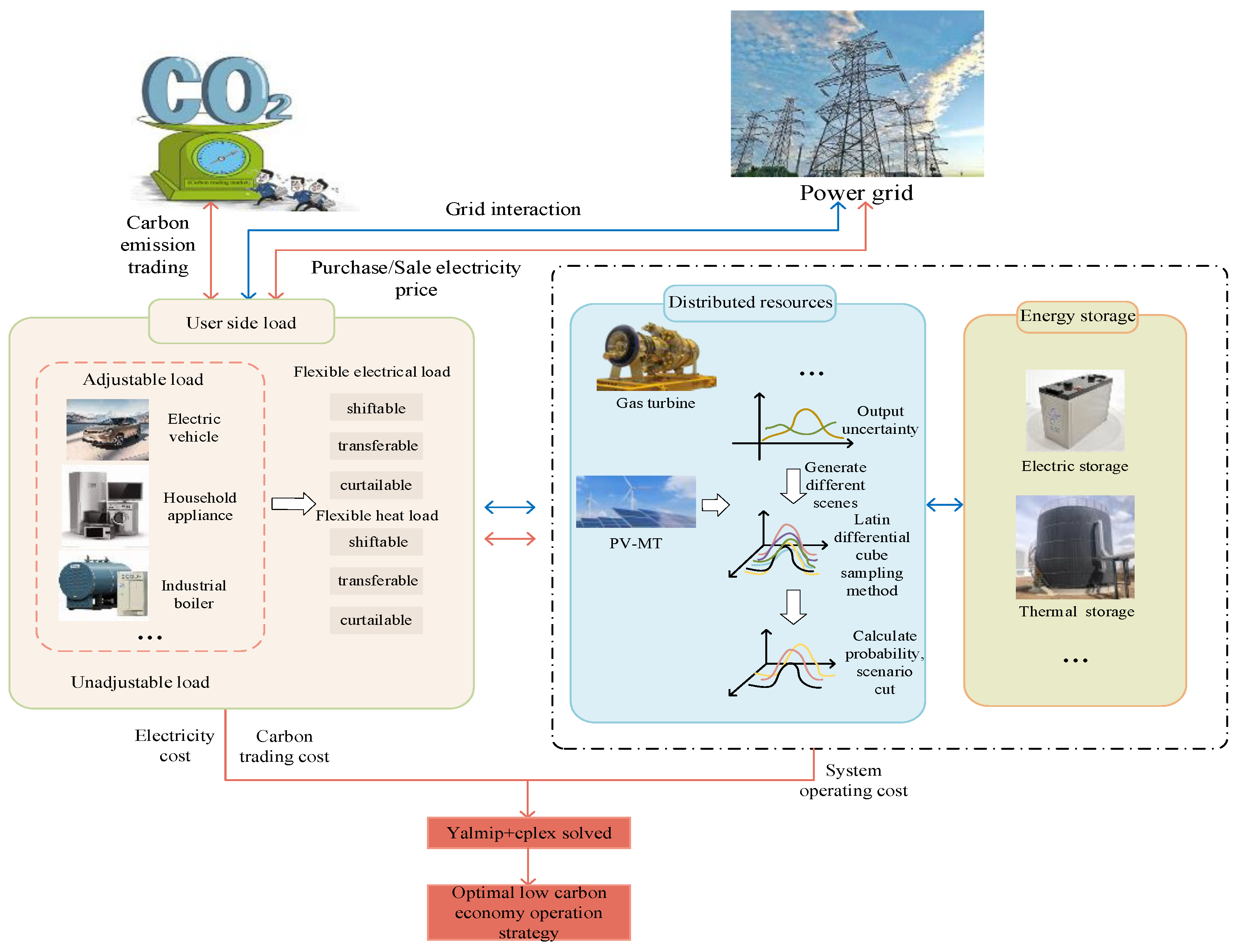
2. LHS-CTM Microgrid Operation System Structure

2.1. LHS-CTM Microgrid System Operation Process

This paper conducts research on the optimal scheduling of an LHS-CTM microgrid system. In the Figure 1, the adjustable load, distributed power supply, and energy storage processing methods are introduced, and the relationship between the microgrid, carbon trading market, and grid is established. In the end, the comprehensive cost is used as the objective function to solve the model. The details are as follows. Firstly, the system is divided into three parts: market, power grid, and microgrid (including user-side load, distributed power supply, and energy storage). The microgrid resources are preprocessed according to energy types. Secondly, the paper establishes the energy and information interaction relationships between the microgrid and the market, as well as the power grid. Finally, by establishing and solving the optimal scheduling model, the optimal low-carbon economic operation strategy can be obtained.

In terms of resource preprocessing, user-side loads are divided into adjustable loads and non-adjustable loads. Adjustable loads include flexible loads, such as electric vehicles, household appliances, and industrial electric furnaces, while non-adjustable loads are rigid loads with high complexity or necessity of adjustment. Adjustable loads can be further classified into flexible electrical and heat loads, which can all be categorized as shiftable, transferable, and curtailable loads based on their demand response characteristics. Distributed power sources are divided into gas turbines and wind–solar power units. Due to the uncertainty of wind and solar energy, the Latin hypercube sampling method is used to generate multi-scenario samples, from which reduced scenarios are selected to predict the power generation of wind–solar power units. Energy storage is divided into thermal storage and electrical storage based on its characteristics.

In terms of interaction relationships, the electricity required by the user-side load is provided by power supply resources, which are divided into two major categories: distributed power sources and energy storage. Gas turbines and wind–solar power units, as distributed power sources, supply electricity to the loads. At the same time, energy storage includes electrical storage and thermal storage, which play a compensatory role when distributed power sources are insufficient. The power grid participates in the electricity trading of the power system by regulating the prices of electricity purchase and sale. In terms of carbon trading, the user-side load chooses to purchase or sell carbon emission rights from the carbon trading market based on their actual carbon emissions from their own equipment.

In terms of the optimal scheduling model, by establishing a comprehensive objective cost function that includes the costs of electricity purchase and sale in the microgrid, carbon transaction costs, and microgrid operation costs, the problem is solved by using Yalmip+Cplex. To demonstrate the advantages of the proposed algorithm, the paper compares different scenarios and algorithms. The following is an elaboration of the theoretical knowledge utilized in this paper.

2.2. Carbon Emissions Market Trading Mechanism

To promote greenhouse gas emission reduction, international policy documents have been issued stipulating that the emission rights of greenhouse gases such as carbon dioxide can be traded as a commodity. This trading mechanism is known as the carbon emissions trading mechanism. Each emitting entity is allocated a certain quota. If an entity’s emissions are lower than the allocated quota, it can sell the surplus quota in the carbon emissions market; if an entity’s emissions exceed the allocated quota, it needs to purchase an additional quota from the carbon emissions market. The trading price of carbon quotas varies with the supply and demand of carbon quotas in the carbon trading market; Formula (1) provides the calculation of the carbon trading price.

$${\omega }_{car}=\left\{\begin{array}{c}\omega {}_{car}{}^{low},Q_{car}\le -l\hfill \\ \\ {\omega }_{car}^0(1+\mu Q_{car}), \left|Q_{car}\right|\le l\hfill \\ \\ {\omega }_{car}^{high}, Q_{car}\ge l\hfill \end{array}\right.$$

(1)

In this formula, ${\omega }_{car}$ represents the carbon trading price; $\omega {}_{car}{}^{low}$ represents the minimum carbon price set by the carbon trading market; ${\omega }_{car}^{high}$ represents the maximum carbon price set by the carbon trading market; ${\omega }_{car}^0$ represents the base carbon price set by the carbon trading market; $Q_{car}$ represents the trading volume of carbon quotas (positive values indicate carbon purchases; negative values indicate carbon sales); $\mu$ represents the carbon price growth rate.

In the market, some bidding will not be accepted; the main reason is the price of the carbon emission quota. Therefore, the clearing rate of carbon emissions trading rights is established to reflect the volatility of the market. First, there is a guide price in the carbon trading market, which is related to the current supply and demand relationship. When the demand for carbon emissions increases, the guide price will decrease and vice versa. Secondly, for the sale of carbon emission rights, enterprises can independently choose the sale price, and the clearance rate of the sale price is related to the guide price; the closer the clearance rate is, the higher the clearance rate. Finally, for the purchase of carbon emission rights, enterprises can independently purchase according to the market price. According to reference [18], the clearing rate of carbon emission trading rights is as shown in Formula (2).

$${\vartheta }_i=({\displaystyle \frac{c_i^s}{{\omega }_{car}}}{\tau }_{car}^s+{\displaystyle \frac{c_i^b}{{\omega }_{car}}}{\tau }_{car}^b){\delta }_i$$

(2)

In this formula, ${\vartheta }_i$ represents the clearing rate of carbon emission trading rights; $c_i^s$, $c_i^b$, respectively, represent the prices of the enterprise’s sale and purchase of the carbon emissions quota; ${\omega }_{car}$ represents the guide price in the market; ${\tau }_{car}^s$, ${\tau }_{car}^b$, respectively, represent the sell and buy coefficient of supply and demand, which is the proportional coefficient of demand and supply; ${\delta }_i$ represents the credit coefficient of the enterprise’s carbon trading market.

2.3. Latin Hypercube Sampling

Latin hypercube sampling (LHS) is a method for randomly sampling from multivariate parameter distributions. By improving the sampling strategy, LHS can achieve higher sampling accuracy with a smaller sampling size. In power system analysis, this method can effectively simulate the uncertainty of wind power output by efficiently generating representative points within the sample space, demonstrating significant advantages in accuracy and efficiency compared to the traditional Monte Carlo methods.

The specific steps of this method can be divided into two parts: Step 1, stratification. Stratify the input variables by dividing the value range of each component into the same intervals to ensure randomness and uniformity of the samples, reducing the correlation between input variables. Step 2, sampling. Sample the stratified input variables to ensure that the confidence intervals are fully covered by the sampling points. For example, let X_k (k = 1, 2, …, K) be any random input variable with a probability distribution function; its probability distribution function is Y_k = F_k(X_k), Here, N represents the sampling size. It divides the ordinate of the probability distribution function into N equal, non-overlapping intervals, each with a length of 1/N. It selects the midpoint of each interval as the value of Y_k, and then calculates the sampled value of X_k using the inverse function method. Finally, the sampled values of Latin hypercube sampling and the K × N sampling matrix can be obtained, as shown in Formulas (3) to (4).

$$X_{kn}={F_k}^{-1}\left({\displaystyle \frac{n-0.5}{N}}\right)\hspace{1em} n=\mathrm{1,2},\cdots ,N$$

(3)

$$X_{KN}=\left(\begin{array}{ccc}{X}_{11}& \dots & X_{1N}\\ ⋮& \ddots & ⋮\\ X_{K1}& \cdots & X_{KN}\end{array}\right)$$

(4)

In the formula, X_KN represents the sampling matrix; X_kn represents the inverse function calculation.

3. Optimization Model Considering Demand Response

3.1. Adjustable Load Characteristics

Adjustable loads can be classified into two types based on their characteristics: flexible electrical load and flexible heat load. Both types of flexible loads are modeled using demand response characteristics. The adjustable load outputs in this region are represented by Formulas (5) to (8):

$$\tilde{P}(t)=\sum _{i=1}^m{X}_i\left(t\right)+M_i\left(t\right)+C_i\left(t\right)$$

(5)

$$T_i^X\in (t_1,t_2)\cup (t_3,t_4)\cup ...\cup (t_{n-1},t_n)$$

(6)

$$T_i^M\in (t_1,t_2)\cup (t_3,t_4)\cup ...\cup (t_{m-1},t_m)$$

(7)

$$\mathsf{\Delta }C(t)=\sum _{i=1}^N{\delta }_i{C}_i\left(t\right)$$

(8)

In this formula, $\tilde{P}\left(t\right)$ represents the total adjustable load power in this region; $X_i\left(t\right)$ represents the power of the ith transferable load; $M_i\left(t\right)$ represents the power of the shiftable load; $C_i\left(t\right)$ represents the power of the curtailable load; $T_i^X$, $T_i^M$, respectively, represent the shiftable and transferable intervals for shiftable and transferable load; $\mathsf{\Delta }C\left(t\right)$ represents the load curtailment at the time t; ${\delta }_i$ represents the reduction ratio of the ith device.

3.2. Characteristics of Distributed Generation

In the microgrid system discussed in this paper, the distributed generation sources include wind–solar power units, gas turbines, and other equipment. Among them, renewable energy sources such as wind and solar are significantly influenced by weather conditions; thus, they exhibit randomness and geographical variability. Relying solely on day-ahead PV and wind power output curves for analysis would lead to unreliable results. Therefore, this paper employs the Latin hypercube sampling (LHS) method to handle the uncertainty in wind and solar power output, enhancing the effectiveness of wind and PV output curves.

Initially, it is necessary to obtain the probability distribution functions (PDFs) for wind turbines and PV systems. Normal distributions are used to simulate the uncertainty in wind and PV output, with their PDFs represented by Formulas (9) and (10).

$$F_p\left(P_{p,t}\right)={\displaystyle \frac{1}{\sqrt{2\pi }{\sigma }_p}}{\displaystyle \underset{-\infty }{\overset{P_{w,t}}{\int }}\exp \left(-\frac{{\left(P_{p,t}-{\mu }_p\right)}^2}{2{{\sigma }_p}^2}\right)}$$

(9)

$$F_w\left(P_{w,t}\right)={\displaystyle \frac{1}{\sqrt{2\pi }{\sigma }_w}}{\displaystyle \underset{-\infty }{\overset{P_{w,t}}{\int }}\exp \left(-\frac{{\left(P_{w,t}-{\mu }_w\right)}^2}{2{{\sigma }_w}^2}\right)}$$

(10)

In this formula, P_p,t, P_w,t represent the output power of the photovoltaic (PV) and wind power generation units at time t; μ_p, σ_p represent the mean and variance of the prediction error for photovoltaic (PV) power; and μ_w, σ_w represent the mean and variance of the prediction error for wind power.

According to the LHS method described by Formulas (11) and (12), the nth sample values for the wind turbine and photovoltaic system can be expressed as

$$P_{p,n}={F_p}^{-1}({\displaystyle \frac{n-0.5}{N}})\hspace{1em}n=\mathrm{1,2},\cdots ,N$$

(11)

$$P_{w,n}={F_w}^{-1}({\displaystyle \frac{n-0.5}{N}})\hspace{1em}n=\mathrm{1,2},\cdots ,N$$

(12)

By utilizing the probability distribution functions to perform reduced sampling on the matrix and finally performing a weighted summation of the sampled values, the resulting output vectors for the wind turbine and photovoltaic system are obtained $P_{pt}=\left(P_{p,1},P_{p,2},\cdots ,P_{p,N}\right)$, $P_{wt}=\left(P_{w,1},P_{w,2},\cdots ,P_{w,N}\right)$.

3.3. Energy Storage Characteristics

Energy storage is a flexible electrical device that can serve as a power source to supply adjustable loads and can also act as a load to absorb wind and solar energy. It can enhance energy utilization efficiency and ensure the stable operation of the power system. Its charging and discharging characteristics are shown in Formula (13).

$$P^{E,H}=\left\{\begin{array}{c}{P}_{cha}^{E,H}, P^{E,H}<0 \mathrm{a}\mathrm{n}\mathrm{d} {\delta }_{cha}=1\\ \\ P_{dis}^{E,H}, P^{E,H}\ge 0 \mathrm{a}\mathrm{n}\mathrm{d} {\delta }_{dis}=1\end{array}\right.$$

(13)

In this formula, P^E,H represents the energy storage power; when P^E,H is negative, it acts as a load to absorb electrical energy; when P^E,H is positive, it acts as a power source to provide electrical energy; P_cha^E,H represents the charging power of the energy storage; P_dis^E,H represents the discharging power of the energy storage; ${\delta }_{cha}$, ${\delta }_{dis}$ are the state variables for the charging and discharging of the energy storage, and ${\delta }_{cha}+{\delta }_{dis}\le 1$.

4. Model Solving Method

4.1. Objective Function

Total cost:

$$Z=C_{bs\_grid}+C_{pw\_om}+C_{fu\_gas}+C_{sto\_om}+C_{dr}+C_{c{o}_2}$$

(14)

In the formula, C_{bs_grid} represents the cost of electricity sales and purchases; C_{pw_om} represents the operation and maintenance cost of wind and solar power equipment; C_{fu_gas} represents the fuel cost; C_{sto_om} represents the operation cost of energy storage; C_dr represents the demand response compensation cost; and $C_{c{o}_2}$ represents the carbon trading cost.

Grid interaction costs:

$$C_{bs\_grid}=c_{buy}{P}_b+c_{sell}{P}_s$$

(15)

O&M costs of wind and solar equipment:

$$C_{pw\_om}=\sum _{i,j=1}^{n,m}{w}_i^p{P}_i^{pv}+w_j^w{P}_j^{wt}$$

(16)

Fuel costs:

$$C_{fu\_gas}=c_{gb}+c_{mt}=\sum _{i=1}^n{\displaystyle \frac{w_i^{gb}{P}_i^{gb}+\epsilon w_i^{mt}{P}_i^{mt}}{\eta }}$$

(17)

Energy storage operating costs:

$$C_{sto\_om}=c_{elec}+c_{heat}=\sum _{i=1}^n{w}_{sto}(P_i^{ech\arg e}+P_i^{edisch\arg e}+P_i^{hch\arg e}+P_i^{hdisch\arg e})$$

(18)

Demand response compensation cost:

$$C_{dr}=c_x^i(P_{shif}+P_{tran}+P_{cut}+P_{Hshif}+P_{Htran}+P_{Hcut})$$

(19)

Carbon trading costs:

$$C_{c{o}_2}=(M_{c{o}_2}-N_{c{o}_2})w_{c{o}_2},M_{c{o}_2}=m_{c{o}_2}^i{P}_i$$

(20)

In the formula, $c_{sell}$, $c_{buy}$, $P_b$, $P_s$ are, respectively, the electricity sales and purchase prices of the power grid and their corresponding quantities; $P_i^{pv}$, $P_j^{wt}$, $w_i^p$, $w_j^w$ are, respectively, the photovoltaic power generation and operating costs of the ith device and the wind power generation and operating costs of the j equipment; $c_{gb}$, $c_{mt}$ are, respectively, gas boiler costs and gas turbine fuel costs; $w_i^{gb}$, $w_i^{mt}$, $P_i^{gb}$, $P_i^{mt}$ are, respectively, the cost factor of the ith gas boiler, the gas turbine gas, and its electricity consumption; $\epsilon$, $\eta$ are, respectively, the power–gas conversion coefficient of the gas boiler and gas turbine; $c_{elec}$, $c_{heat}$ are, respectively, the operating costs of electric energy storage and thermal energy storage; $P_i^{ech\arg e}$, $P_i^{edisch\arg e}$, $P_i^{hch\arg e}$, $P_i^{hdisch\arg e}$, $w_{sto}$ correspond, respectively, to the amount of electricity in the charging and discharging of the ith device electric energy storage and thermal energy storage and the cost coefficient of the operation and maintenance of the energy storage device; $c_x^i$ represents the demand response subsidized price; $P_{shif}$, $P_{tran}$, $P_{cut}$, $P_{Hshif}$, $P_{Htran}$, $P_{Hcut}$ are, respectively, the shiftable, transferable, and interruptible loads corresponding to the electrical load and the thermal load; $M_{c{o}_2}$, $N_{c{o}_2}$ are, respectively, the MG carbon emissions and the carbon emissions quota; $w_{c{o}_2}$, $P_i$, $m_{c{o}_2}^i$ are, respectively, the carbon emissions trading price, electricity consumption of the ith device, and its carbon emissions coefficient.

4.2. Constraints

1. The constraints of the electrical and thermal energy storage:

$$\{\begin{array}{l}{P}_{\min }^{E,H}\le P_i^{E,H}(0)\le P_{\max }^{E,H}\\ -P_{cs}^{E,H}\le P_i^{E,H}(t)\le P_{cs}^{E,H}\\ T_{ch}+T_{disch}\le T_{\max }^{E,H}\end{array}$$

(21)

In the formula, $P_i^{E,H}(0)$, $P_{\max }^{E,H}$, $P_{\min }^{E,H}$ are, respectively, the initial energy storage of the electric energy (thermal) storage and its corresponding upper and lower energy storage limits devices; $P_i^{E,H}(t)$, $P_{cs}^{E,H}$ are, respectively, the electric (thermal) energy storage device charge/discharge (thermal) power and maximum power; $T_{ch}$, $T_{disch}$, $T_{\max }^{E,H}$ are, respectively, the charge/discharge (thermal) time and equipment lifetime of the electric (thermal) energy storage device.

2. The constraints of distributed power:

$$\{\begin{array}{l}0\le P_i^{pv}\le P_{\max }^{pv}\\ 0\le P_i^{wt}\le P_{\max }^{wt}\\ 0\le P_i^{mt}\le P_{\max }^{mt}\\ 0\le P_i^{gb}\le P_{\max }^{gb}\end{array}$$

(22)

$$\begin{array}{c}if\begin{array}{c}\end{array}{P}_s=P-(P_i^{pv}+P_i^{wt}+P_i^{mt}+P_i^{gb})<0,c_{sell}=0\\ else,c_{buy}=0\end{array}$$

(23)

In the formula, $P_{\max }^{pv}$, $P_{\max }^{wt}$, $P_{\max }^{gb}$, $P_{\max }^{mt}$ are, respectively, photovoltaic, wind, gas boiler, and gas turbine maximum output power.

3. Adjustable load constraints

Shiftable electrical/thermal load:

$$\{\begin{array}{l}{T}_{shif}(t_1,t_2)\le T_{shif,\max }\\ P_{ashif}(t_1,t_2)=P_{shif}\\ t_1\le t_{\min }\\ t_2\le t_{\max }\end{array}$$

(24)

In the formula, $T_{shif}(t_1,t_2)$, $T_{shif,\max }$ are, respectively, t₁~t₂ shiftable period and maximum shiftable time; $P_{ashif}(t_1,t_2)$ is shiftable quantity; $t_{\min }$, $t_{\max }$ are, respectively, the initial time and end time of the shiftable period.

Transferable electrical/thermal load:

$$\{\begin{array}{l}{T}_{i,\min }^{tran}\le T_{tran}(t_1)\le T_{i,\max }^{tran}\\ P_{atran}(t_1,t_2)=P_{tran}\end{array}$$

(25)

In the formula, $T_{tran}\left(t_1\right)$, $T_{i,\min }^{tran}$, $T_{i,\max }^{tran}$ are, respectively, the t₁ transfer time point and the upper and lower limits of the ith transferable time period; $P_{atran}$ is the transferable quantity.

Curtailable electrical/thermal load:

$$\{\begin{array}{l}{T}_{i,\min }^{cut}\le T_{cut}(t_1)\le T_{i,\max }^{cut}\\ N_{cut}\le N_{\max }\\ 0\le {\tilde{P}}_{cut}(t_1)\le \lambda P_{cut}(t_1)\end{array}$$

(26)

In the formula, $T_{cut}\left(t_1\right)$, $T_{i,\min }^{cut}$, $T_{i,\max }^{cut}$ are, respectively, the t₁ curtailable time point and the upper and lower limits of the ith curtailable time period; N_cut, N_max are, respectively, the number of cuts and the maximum number of cuts; ${\tilde{P}}_{cut}(t_1)$, $P_{cut}\left(t_1\right)$, $\lambda$ are, respectively, the reduction amount, load amount, and reduction ratio at the moment of t₁;

4. Electric equilibrium constraint

$$P_s+P_b+P_i^{pv}+P_i^{wt}+P_i^{mt}-P_i^{ech\arg e}+P_i^{edisch\arg e}={\tilde{P}}_e+{\tilde{P}}_{eshif}+{\tilde{P}}_{etran}-{\tilde{P}}_{ecut}$$

(27)

$${\tilde{P}}_e=P_e-P_{shif}-P_{tran}$$

(28)

$${\omega }_{mt}{P}_i^{mt}+P_i^{gb}-P_i^{hch\arg e}+P_i^{hdisch\arg e}={\tilde{P}}_h+{\tilde{P}}_{Htran}+{\tilde{P}}_{Hshif}-{\tilde{P}}_{Hcut}$$

(29)

$${\tilde{P}}_h=P_h-P_{Htran}-P_{Hshift}$$

(30)

In the formula, $P_e$, $P_h$ are, respectively, the initial electrical and thermal loads; ${\tilde{P}}_e$, ${\tilde{P}}_h$ are, respectively, the basic electrical and thermal loads; ${\tilde{P}}_{eshif}$, ${\tilde{P}}_{etran}$, ${\tilde{P}}_{ecut}$ are, respectively, the electric load after shift and transfer and cut amount; ${\tilde{P}}_{Htran}$, ${\tilde{P}}_{Hshif}$, ${\tilde{P}}_{Hcut}$ are, respectively, the heat load after shift and transfer and cut amount.

5. Example Analysis

5.1. Parameter Setting

Based on the actual case data of a certain place in China, this paper selects detailed parameters covering distributed power supply, energy storage devices, wind, and photovoltaic power generation systems. These parameters are not only representative in China, but also have wide applicability in the international scope due to their universality and technical characteristics. In view of the globalization trend of the carbon emissions trading market and the widespread adoption and implementation of the demand response mechanism in the world, the algorithm and analysis results used in this paper can provide strong support for the optimization of the energy system in the context of China, and they can also show an important reference value for the exploration of the international energy transition and the low-carbon development path. Therefore, it is proved that the algorithm is highly applicable and forward-looking at the international level. The details are as follows.

This paper selects the real historical data of a place for simulation; As shown in

Table 1. Valley peak TOU price and sell price.

Time Period	Buy Price [¥/kW·h]	Sell Price [¥/kW·h]
00:00–7:00	0.25	0.25
7:00–10:00	0.53	0.42
15:00–18:00
21:00–00:00
10:00–15:00	0.82	0.65
18:00–21:00

, the TOU pricing of Shaanxi Province in China is selected in this paper. The scheduling period is 24 h, the parameters of the energy storage and other equipment are referenced [19]; the details of the parameters are shown in

Table 2. Operating parameters of units.

Generator	Lower Limit [kW]	Upper Limit [kW]	Running Cost [¥/kW·h]
PV	0	Predicted value	0.52
WT	0	Predicted value	0.72
Gas boiler	0	100	Natural gas price
Gas turbine	0	200	Natural gas price
Storage	45	95	0.5

. The charge and discharge efficiency of the energy storage device is set to 90%. The output of photovoltaic and wind power adopts the results obtained by the proposed algorithm. As for changing users’ behavior regarding electricity consumption through the TOU pricing policy, to relieve the pressure of electricity consumption, the TOU pricing ranges based on local conditions are established in different regions according to the peak and valley segments of the local users’ electricity consumption, but all of them are to guide users’ behavior regarding electricity consumption. For the carbon trading market, each enterprise has a rated carbon emissions quota over a period, but an enterprise sometimes does not make full use of it due to unsaturation of production planning or other reasons. Therefore, there are some enterprises that sell the carbon emissions quota that they cannot use up. According to the equipment in the selected area, the carbon emissions and quota coefficients of the equipment are listed in the

Table 3. Carbon emission coefficient and quota coefficient.

Power	Carbon Emission Coefficient [g/(kW·h)]	Quota Coefficient [g/(kW·h)]
PV	43.0	78.0
WT	154.5	78.0
Coal power	1303.0	798.0
Natural gas	564.7	424.0
Storage	91.3	0

. In order to encourage enterprises to actively participate in the carbon trading market through price, the carbon trading price changes with the demand for carbon trading. The carbon emissions trading price range is 100–200 ¥/t (1 CNY¥ ≈ 0.14 USD$).

In this paper, the MATLAB platform (https://www.mathworks.com/products/matlab.html, accessed on 2 August 2024) Yalmip+cplex is used to solve the model. As shown in

Table 4. Load participation in different scenarios.

Scenarios	Flexible Load Participation	Contrast Point
Scenario 1	Flexible electrical and heat load	Operating cost and load interaction
Scenario 2	Only flexible electrical load
Scenario 3	Without flexible load

, in order to show the advantages of flexible load and heat load participating in the distribution network, three scenarios are set up: Scenario 1: the participation of the flexible electrical load and flexible heat load in the system optimization scheduling is considered; Scenario 2 only considers the participation of the flexible electrical load in the system optimization scheduling; Scenario 3: the flexible load is not considered to participate in the system optimization scheduling.

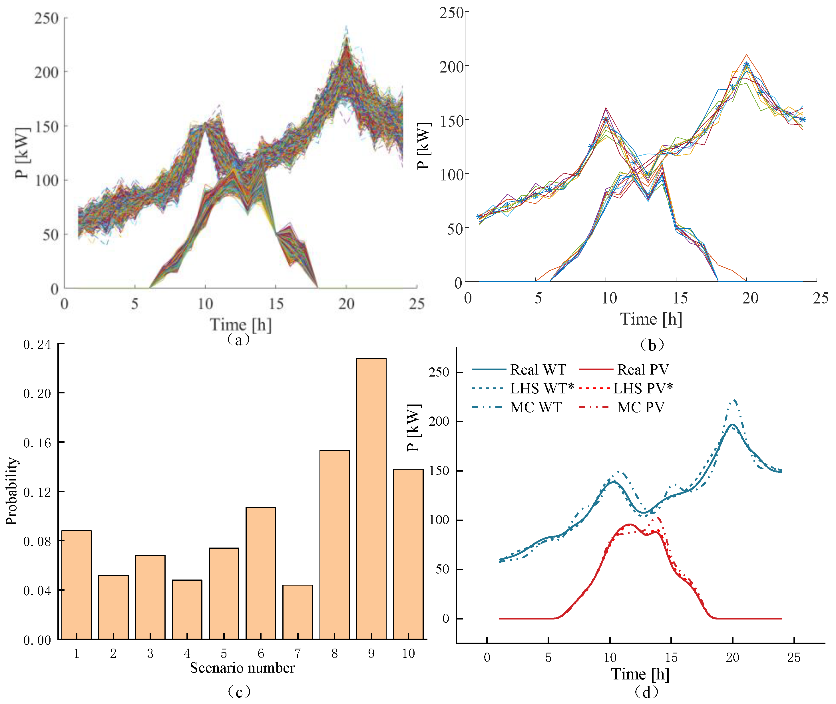
5.2. Analysis of Wind Power Processing Based on LHS

In order to demonstrate the superiority of the proposed algorithm, the Monte Carlo method based on probabilistic distance reduction is established to compare with the proposed algorithm. Figure 2a–c shows the uncertainty of the wind power output of the LHS algorithm. Therefore, stratified sampling technology is used to divide the sampling interval into different layers according to the mean and covariance; then, independent and random sampling from different layers can effectively improve the sampling accuracy. Finally, this paper uses this method to generate 1000 scenes and then retains the scene with the highest probability and finally reduces it to 10 scenes. According to the probability, the weighted sum is carried out to obtain the final PV and wind power output curves.

Figure 2d shows the comparison between the results of the proposed algorithm and the Monte Carlo method, from the loads at 10:00 and 22:00. Compared with the real data, the MC algorithm has an error of about 10 kW, which will have a great impact on the subsequent optimization scheduling work. However, the average error of the algorithm in this paper is less than 5%, and the accuracy of the simulation and prediction of the wind power and photovoltaic power is higher. Therefore, the photovoltaic and wind power output results obtained by the algorithm in this paper are more suitable for the current scenario than that obtained by the Monte Carlo method.

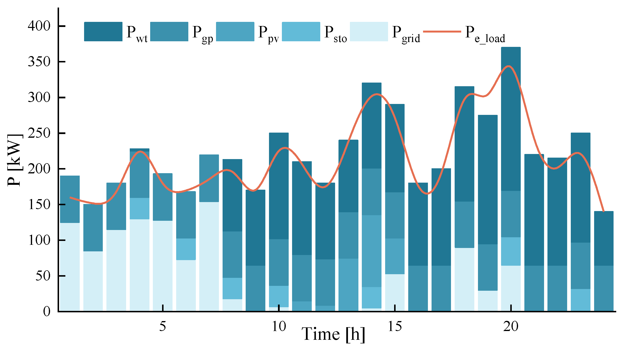
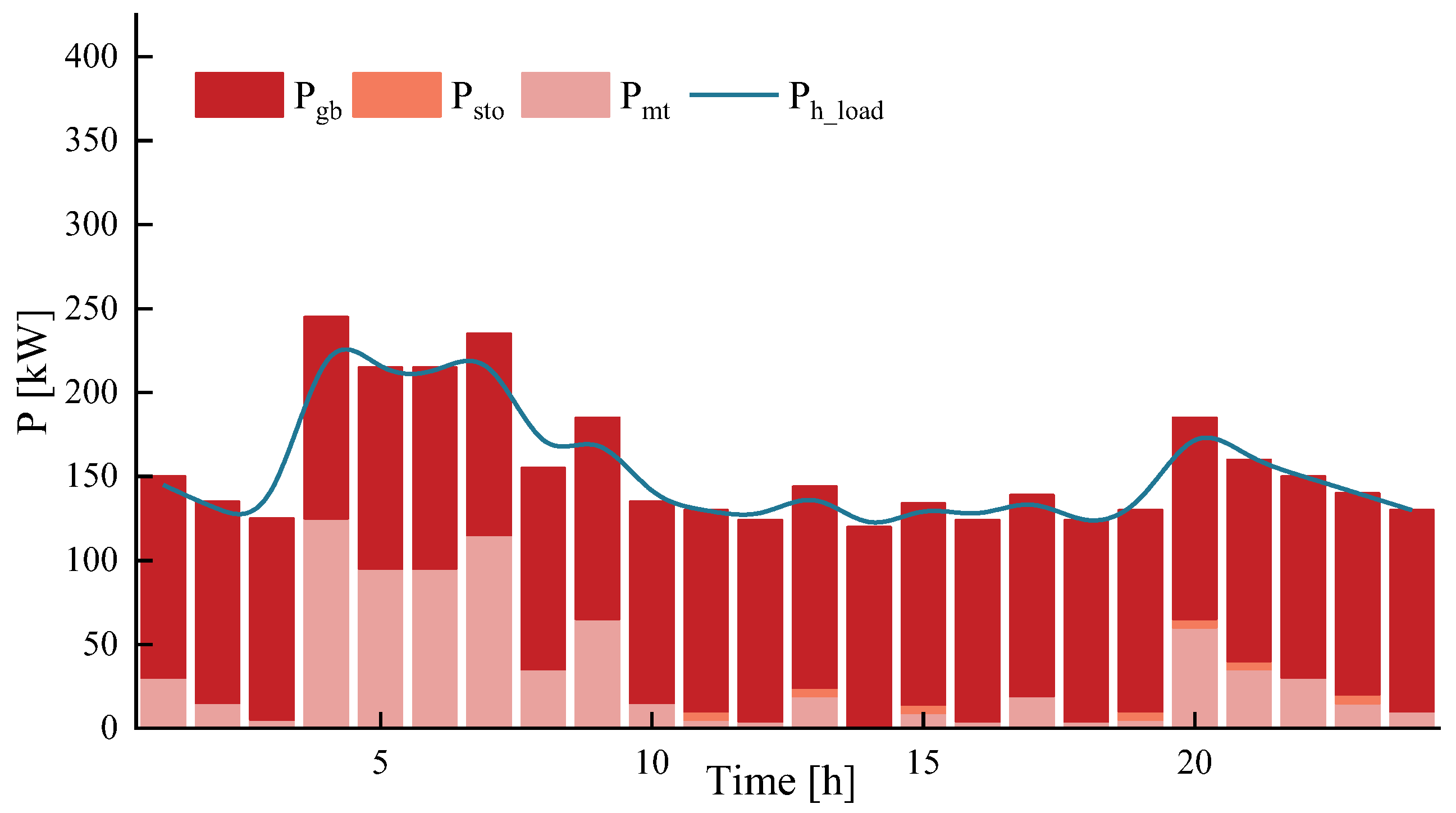
5.3. Low-Carbon Economy Optimal Scheduling Results

After solving the model with MATLAB, the optimization results of the three scenarios established in this paper can be obtained. Among them, the power distribution of the electricity and heat load corresponding to scenario 1 are shown in Figure 3 and Figure 4. The comparison of the electricity and heat load before and after participating in the demand response is shown in Figure 5. The total amount of carbon trading in scenario 1 is showed in Figure 6

In Figure 3, the blue columns from dark to light are wind power output, gas boiler output, photovoltaic output, energy storage output, and grid interaction. The red line is the electrical load demand, for electrical load. Then, in the period from 7:00 to 12:00, because the electricity price is in the valley segment, the electricity price is only 0.25 ¥/kW·h, the operation cost of power generation and energy storage equipment, such as gas turbines and wind power, is high, and the PV cannot be produced due to no light; so, the priority is to purchase electricity from the grid in this period. In order to meet the power balance, part of the power load is compensated by wind power and the gas boiler. From the wind power, the PV output curves. In the period from 7:00 to 12:00, the wind power generation output is at the top of one of the PV output’s gradually increasing stages, and distributed energy is abundant; in order to ensure the comprehensive cost, the electricity price in this period is in the flat segment and the peak segment, and the power purchase price is high; therefore, the photovoltaic output is the highest in this part, followed by gas turbines and photovoltaic power, with almost no power purchase from the grid. In the period from 12:00 to 23:00, the demand for electricity load and wind power resources gradually increases, making full use of scenery resources and gas turbines to compensate; at the peak electricity price in the period from 12:00 to 15:00 and 18:00 to 21:00, the battery releases electrical energy, and the battery life is shorter than that of other devices. Therefore, the priority of the battery participating in the grid interaction is lower, and the power load is usually only compensated.

As shown in Figure 4, the red columns from dark to light are gas boiler output, energy storage output, and gas turbine output. The blue line is the electrical load demand. Then, the heat load is provided by the gas turbine, thermal energy storage, and gas boiler equipment; it mainly comes from the gas boiler and also has thermal output in its electrical output, so as to reduce the cost of the power dispatch. At the same time, the thermal energy storage and gas boiler carry out secondary combustion. When the heat load rises sharply from 4:00 to 7:00, the gas turbine and the energy storage carry out combustion. During the rest of time, the gas boiler can roughly meet the heat load demand that needs to be met during the operation of the microgrid because the gas boiler is in a full power state during the power output. In order to ensure the life and cost of the thermal energy storage, the rest are compensated by the gas turbine and the thermal energy storage in turn.

In Figure 5, the green line and dotted line are the pre-and post-load curves of the demand response of the electric load; the yellow line and dotted line are the pre-and post-load curves of the demand response of the thermal load, and the red dotted line is the electricity price curve. Then, when the electricity price peaks, both kinds of loads decrease, and the load rises in the valley segment. The results of the participation of the adjustable load resources in the optimal scheduling of the microgrid are shown, including the demand response results of the electrical load and thermal load. In the electricity load, for the electricity price valley segment from 00:00 to 07:00, due to the characteristics of the shiftable load and transferable load, the load in the flat section and peak section of the electricity price is transferred to the valley segment. It is obvious that the load increases by nearly 20 kW at around 6:00, thus reducing the electricity cost. In some flat segment segments, for example, from 7:00 to 10:00, there is also an increase in load capacity, because some transferable and transferable load segments are not in the electricity price valley segment; so, in order to reduce costs, they choose to transfer to the flat segment, and the rest of the electricity price flat segment segments have load reduction. In the peak segment, that is, from 10:00 to 18:00 and from 18:00 to 21:00, there is a certain amount of load reduction in this part, which is the result of the combined action of shiftable, transferable, and curtailable loads. Especially at 12:00, the reduction amount reaches nearly 100 kW. In the thermal load, in a manner similar to the electric load, the load reduction occurs between 11:00 and 21:00 in the interval dominated by the peak price segment, due to the shift and transfer of the flexible load to the flat price segment and the valley segment between 6:00 and 11:00 and the reduction in the load that can be reduced.

In the Figure 6, the green column is the carbon transaction volume, and the carbon transaction volume is the highest in the electricity price valley segment, because the electricity price is low, and the electricity consumption behavior of power users, especially industrial users, shifts in this period. Then, it shows the total amount of carbon trading at each moment, and it can be clearly seen that the carbon trading volume is mainly concentrated between 00:00 and 07:00. The reason is that the price of electricity in the valley is relatively low, encouraging users to consume electricity during this period; industrial users in particular often adjust the production plan in the early morning to reduce the cost of electricity, but the electricity consumption will be accompanied by an increase in carbon emissions; so, the carbon trading volume in this period is higher. Meanwhile, in the carbon trading volume, the clearance rate is more than 97%. The low clearance rate is due to the small number of carbon emission rights sold, and there may be a certain probability of clearance failure.

In order to demonstrate the advantages of flexible load, this paper compares various costs by establishing multiple scenarios; as shown in

Table 5. Cost in different scenarios.

Scenarios	Scenario 1	Scenario 2	Scenario 3
Cgrid_buy	422.4155	458.5074	725.7155
Cgrid_sell	−5.08 × 10−13	−1.69 × 10−13	−1.3401 × 10−13
Cfu_gas	1103.8668	1084.0341	1177.2766
Cpw_om	1352.9341	1365	1419.2324
Csto_om	289.4192	283.7727	289.559
Cdr	−251.7222	−177.4	0
Cco2	143.3098	149.6765	196.353
Z [¥]	3060.2232	3163.5907	3808.1365

, it introduces the corresponding power purchase cost, power sale cost, fuel cost, PV/wind power operating cost, energy storage operating cost, demand response compensation, and carbon trading cost in different scenarios. Compared with scenario 1 and scenario 2, the difference between them lies in the participation of flexible thermal load. The total cost difference between them is about 103 ¥, which is mainly concentrated in the cost of electricity purchase and demand response. The difference is about 40 ¥ and 70 ¥, respectively, because the demand response cost increases due to the absence of flexible thermal load. The reason is the situation regarding the low utilization rate of the heat load and the residual flexible heat load of this part. Compared with scenario 1 and scenario 3, the difference between the two lies in the participation of flexible electrical and thermal loads; so, the total cost difference is nearly 800 ¥, resulting in this result also being concentrated in the power purchase cost and demand response cost. The sum of the two parts reaches nearly 600 ¥, accounting for about 80% of the total cost difference, and the rest is the increase in the carbon emission cost, due to the lack of participation of the flexible loads. It is necessary to meet the power load balance; so, the energy generated in the power generation equipment and energy storage equipment is not used reasonably and effectively, resulting in an increase in the cost of the power purchase, and the increase in power consumption will inevitably increase the cost of the carbon emissions. Therefore, it is necessary to consider the participation of flexible loads in the optimization of microgrid scheduling.

6. Discussion

In most of the cases studied in this paper, based on the current instability of both power supply and demand, it is a more efficient way to use the microgrid to deal with the power supply and demand balance and the consumption of new energy on the spot. This method can improve the stability of the power system and the economy of users, especially when enterprise entities are required to conduct carbon trading markets under the carbon emissions trading mechanism [20,21]. By combining the optimal scheduling and demand response of the microgrid, the characteristics of flexible load are used to guide the power consumption behavior of the power users, which reduces the comprehensive cost of the users and alleviates the power consumption pressure of the power system. There is power generation equipment, such as distributed power supply and energy storage equipment, in the microgrid, and the thermal energy generated by the power generation equipment is rationally utilized. Therefore, the existence of electric load and thermal load is considered in this paper [22,23], and the energy existing in the microgrid is utilized as efficiently as possible. Although the society recognizes that solar photovoltaic and wind power in the microgrid are important green energy sources, randomness still exists in the PV and wind power, and the operation and maintenance costs of PV and wind power equipment are limited. In order to reduce carbon emissions and complete the green transformation of the power system, it is necessary to analyze and study the economic costs and output characteristics [24].

However, the optimal scheduling of microgrids is observed in the context of the model studied in this paper. First, the optimal scheduling of the microgrid is limited by the geographical location of the region. In order to ensure the effectiveness of the proposed algorithm, its applicability should be taken into account [25,26]. If there are specific environmental requirements, there is no need. Second, in order to ensure the stable operation of the microgrid and the stable supply and demand of the power system, it is necessary to evaluate the operation capability of the microgrid. In order to solve the problem that the power grid may be oversupplied after the optimized dispatch of the microgrid is mature, the stable operation cost of the power grid should be included in the model in the future. Third, the uncertainty of wind power and photovoltaic power only needs to be within a reasonable error range and can be compensated by other power generation equipment or energy storage equipment in the power load balance.

During the modeling process, a key observation in this study was that the thermal energy generated by different energy storage devices and power generation devices can be rationally utilized or stored at the same time. For example, in reference [27], electricity is used to generate thermal energy so as to participate in optimal scheduling and demand response. The research results show that the cost of the overall system is reduced. However, unlike their study, the heat generated by the operating equipment is added to the model in this paper, which does not directly use electric energy to generate heat and can greatly reduce the operating cost of the system and alleviate the power grid pressure. At the same time, in the stage of the gradual rise of the carbon trading market, in response to low-carbon policies, adding carbon trading costs to the model can also guide the model of power users’ consumption behavior. Therefore, due to the economic costs and social benefits, the establishment of the model and the influence of factors on the research results have a significant impact on the optimization of microgrid scheduling.

7. Conclusions

This study established a microgrid optimization dispatch model based on LHS-CTM, with the goal of achieving the optimal low-carbon economic cost for the microgrid while meeting the electric and thermal load requirements of the microgrid. The results highlight that:

• In the case of the randomness of wind power generation and photovoltaic power generation, the accuracy of the output curve prediction is low. In this context, some of the studies use algorithms with higher model complexity to predict it. According to this study, when new energy sources such as photovoltaic power participate in microgrid optimization scheduling, the Latin hypercube sampling method is used to describe the output curve, and the error will not exceed ±5%, which can be compensated by other power generation equipment and energy storage equipment during actual participation.
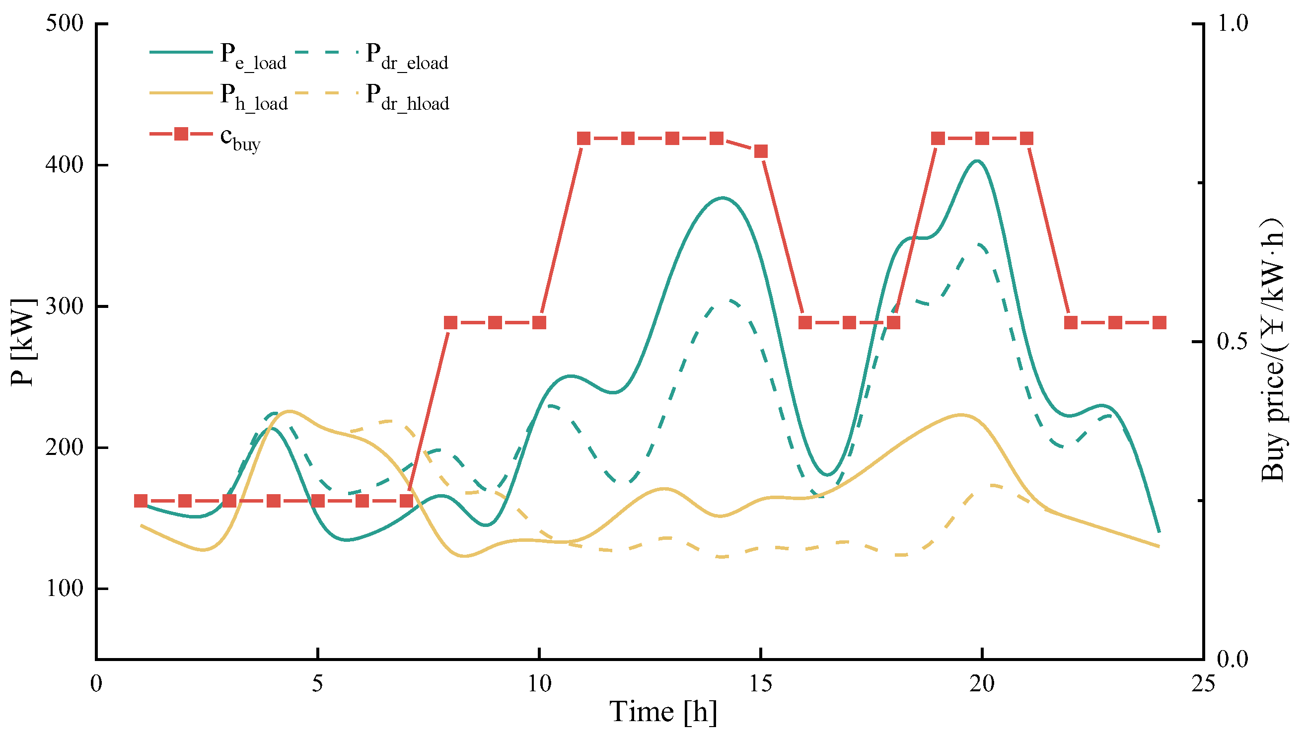
• In the case of flexible loads participating in the optimal scheduling of the microgrid, this study needs to involve both flexible electrical and thermal loads in the optimal scheduling of the microgrid. In addition, some power generation and energy storage devices have thermal energy at the same time as electrical output, and the two kinds of loads can be used to participate in demand response and obtain subsidies. The comprehensive cost of the microgrid will be greatly reduced.
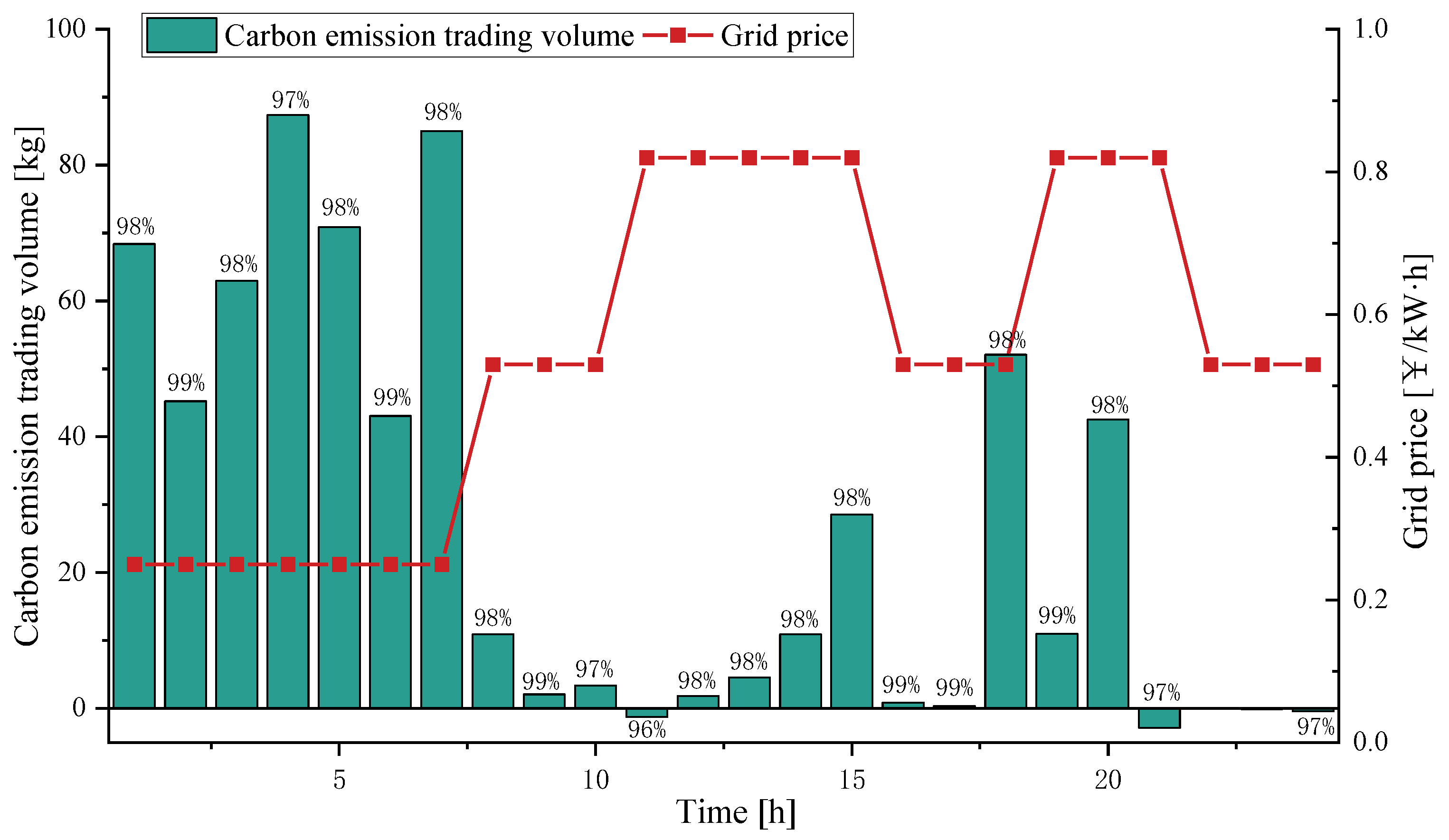
• For the carbon trading market, adding the carbon trading mechanism to the optimal scheduling of microgrids can not only reduce operating costs but also improve social benefits, facilitate carbon reduction policies, and accelerate the green transformation of the power system. However, due to the risk of carbon trading price volatility and the increase in carbon emissions caused by enterprise development, it is necessary to use new energy and energy storage equipment for reasonable planning and operation to reduce comprehensive costs and carbon emissions.

References

1. Han, Y.; Zhang, K.; Li, H.; Coelho, E.A.A.; Guerrero, J.M. MAS-based distributed coordinated control and optimization microgrid and microgrid clusters:a comprehensive overview. IEEE Trans. Power Electron. 2018, 33, 6488–6508. [Google Scholar] [CrossRef]
2. Cao, J.; Jin, Y.; Zheng, T. A decentralized robust voltage control method for distribution networks considering the uncertainty of distributed generation clusters. Power Syst. Prot. Control 2023, 51, 155–166. [Google Scholar]
3. Shi, C.; An, R.; Gao, H.; Jiang, S.; He, S.; Liu, J. Flexible operation method for a distribution network based on flexible multi-state switching and dynamic reconfiguration. Power Syst. Prot. Control 2023, 51, 133–144. [Google Scholar]
4. Yu, Y.; Li, Y.; Chen, S. Distributionally robust optimal dispatch of distribution network considering multiple source-storage coordinated interaction. Electr. Power Eng. Technol. 2021, 40, 192–199. [Google Scholar]
5. Sun, Q.; Yu, X.; Wang, J. Discussion on Challenges and Countermeasures of “Double High” Power Distribution System. Proc. CSEE 2024. Available online: http://kns.cnki.net/kcms/detail/11.2107.tm.20240801.0924.004.html (accessed on 2 August 2024).
6. Yu, H.; Cai, G.; Shi, S.; Zhang, H.; Peng, D.; Yin, S. Operation Optimization Method for Microgrid with Large-scale Charging Piles. Proc. CSU-EPSA 2022, 34, 16–25. [Google Scholar]
7. Xing, Y.; Ren, T. Application research of improved MOPSO in Microgrid optimal dispatch. Acta Energiae Solaris Sin. 2024, 45, 191–200. [Google Scholar]
8. Li, J.; Ju, Y.; Zhang, L.; Liu, W.; Wang, J. Multi-time scale distributed robustoptimal schedulingof microgrid based on model predictive control. Electr. Power Eng. Technol. 2024, 43, 45–55. [Google Scholar]
9. Khatsu, S.; Srivastava, A.; Das, D.K. Solving Combined Economic Emission Dispatch for Microgrid using Time Varying Phasor Particle Swarm Optimization. In Proceedings of the 2020 6th International Conference on Advanced Computing and Communication Systems (ICACCS), Coimbatore, India, 6–7 March 2020; pp. 411–415. [Google Scholar]
10. Sutton, R.S.; Barto, A.G. Reinforcement Learning: An Introduction, 2nd ed.; MIT Press: Cambridge, MA, USA, 2018; pp. 196–205. [Google Scholar]
11. Gao, G.; Yang, S.; Guo, X. A Review of Research on the Application of Deep Reinforcement Learning in Optimization Dispatch of Power Grids with Distributed Flexible Resources. Proc. CSEE 2024, 44, 6385–6404. Available online: http://kns.cnki.net/kcms/detail/11.2107.TM.20240612.1139.002.html (accessed on 6 August 2024).
12. Tang, G.; Wu, H.; Xu, Z.; Li, Z.T. Two-Stage Robust Optimization for Microgrid Dispatch with Uncertainties. In Proceedings of the 2023 6th International Conference on Energy, Electrical and Power Engineering (CEEPE), Guangzhou, China, 21–23 April 2023; pp. 497–502. [Google Scholar]
13. Yang, J.; Ma, P.; Li, L. Two-stage Distributed Robust Energy Storage Capacity Optimization Method for Large-scale Wind Power Access to Microgrid. J. Electr. Eng. 2024. Available online: http://kns.cnki.net/kcms/detail/10.1289.TM.20240322.0945.002.html (accessed on 6 August 2024).
14. Pan, J.; Lu, Y.; He, B.; Zhang, X.; Yu, Z.W.; Zhang, X.Z.; Ma, J.H. Research on economic dispatch of microgrid considering uncertainty of wind and solar output. Adv. Technol. Electr. Eng. Energy 2024, 43, 56–64. [Google Scholar]
15. Duan, F.; Eslami, M.; Khajehzadeh, M.; Basem, A.; Jasim, D.J.; Palani, S. Optimization of a photovoltaic/wind/battery energy-based microgrid in distribution network using machine learning and fuzzy multi-objective improved Kepler optimizer algorithms. Sci. Rep. 2024, 14, 13354. [Google Scholar] [CrossRef]
16. Wang, S.; Yue, Y.; Cai, S.; Li, X.; Chen, C.; Zhao, H.; Li, T. A comprehensive survey of the application of swarm intelligent optimization algorithm in photovoltaic energy storage systems. Sci. Rep. 2024, 14, 17958. [Google Scholar] [CrossRef]
17. Yang, X.; Ye, X.; Li, Z.; Wang, X.; Song, X.; Liao, M.; Liu, X.; Guo, Q. Hybrid energy storage configuration method for wind power microgrid based on EMD decomposition and two-stage robust approach. Sci. Rep. 2024, 14, 2733. [Google Scholar] [CrossRef] [PubMed]
18. Liang, N.; Miao, M.; Xu, H. Bi-Level Optimal Scheduling of Integrated Energy System Considering Green Certificates-Carbon Emission Trading Mechanism. Acta Energiae Solaris Sin. 2024, 45, 312–322. [Google Scholar]
19. Liu, R.; Li, Z.; Yang, X.; Sun, G.; Li, L. Optimal Dispatch of Community Integrated Energy System Considering User-Side-Flexible LOAD. Acta Energiae Solaris Sin. 2019, 40, 2842–2850. [Google Scholar]
20. Duan, S.; Jiang, X.; Shang, J. Rolling Clearing Model of Electric Carbon Joint Market Based on Centralized Carbon Trading Mechanism. In Proceedings of the 2023 IEEE 7th Conference on Energy Internet and Energy System Integration (EI2), Hangzhou, China, 15–18 December 2023; pp. 3199–3205. [Google Scholar]
21. Deng, W.; Dai, Z.; Lu, C. Research on Output Forecasting of Wind Power and Photovoltaic Complementary Power Plant Based on Adaptive Neural Network. Autom. Instrum. 2024, 97–100+105. [Google Scholar]
22. Zhong, M. Multi-Objective Optimal Scheduling of Microgrid Considering Wind and Solar Power Uncertainty and Demand Side Management. Master’s Dissertation, Wuhan University, Wuhan, China, 2022. [Google Scholar]
23. Ye, L.; Li, J.; Lu, P. Wind Power Time Series Aggregation Approach Based on Affinity Propagation Clustering and MCMC Algorithm. Proc. CSEE 2020, 40, 3744–3754. [Google Scholar]
24. Guo, W.; Wang, G.; Min, Y. Hybrid Energy Storage Capacity Configuration for Traction Power Supply Systems Considering Ladder-type Carbon Trading Mechanism. J. Southwest Jiaotong Univ. 2024. Available online: http://kns.cnki.net/kcms/detail/51.1277.U.20240719.0942.004.html (accessed on 7 August 2024).
25. Keshta, H.E.; Hassaballah, E.G.; Ali, A.A.; Abdel-Latif, K.M. Multi-level optimal energy management strategy for a grid tied microgrid considering uncertainty in weather conditions and load. Sci. Rep. 2024, 14, 10059. [Google Scholar] [CrossRef]
26. Xu, Y.; Duan, J. Study on joint control of integrated energy microgrid based on stepped carbon trading. Therm. Power Gener. 2024, 53, 105–115. [Google Scholar]
27. Wang, R. Optimization Operation Strategy of Carbon Capture Power Plant and Flexible Load Collaborative Consumption of Wind Power. Master’s Thesis, Northeast Electric Power University, Jilin, China, 2024. [Google Scholar]
Figure 1. LHS-CTM microgrid system operation process.
Energies 17 04633 g001
Figure 2. Based on LHS WT-PV output result. (a) Based on LHS WT-PV scene generation; (b) based on LHS WT-PV scene reduction; (c) based on LHS WT-PV scene probability; (d) comparison of different methods; “*” represented the algorithm used in this paper.
Energies 17 04633 g002
Figure 3. The electric load balances the output of each unit.
Energies 17 04633 g003
Figure 4. The heat load balances the output of each unit.
Energies 17 04633 g004
Figure 5. Demand response electrical and thermal load curves.
Energies 17 04633 g005
Figure 6. Carbon trading volume.
Energies 17 04633 g006