Optical Investigation of Sparks to Improve Ignition Simulation Models in Spark-Ignition Engines

Abstract

The use of renewable fuels in place of fossil fuels in internal combustion engines is regarded as a viable method for achieving zero-impact-emission powertrains. However, to achieve the best performance with these fuels, these engines require further optimization, which is achieved through new combustion strategies and the use of advanced ignition systems such as prechambers. Since simulations greatly accelerate this development, accurate simulation models are needed to accurately predict the combustion phenomenon, which requires a deep understanding of the ignition phenomenon as it significantly affects combustion. This work presents a comprehensive experimental methodology to study sparks under engine conditions, providing quantitative data to improve and validate ignition simulation models. The goal was to determine the volume generated by sparks under engine conditions that can initiate combustion and use this information to improve simulation results to match the experimental results. The visible sparks were observed with high-speed cameras to understand their time-resolved evolution and interaction with the flow. The heat transfer from the plasma was also visualized using a modified Background-Oriented Schlieren technique. The information gained from the experimental observations was used to improve an ignition simulation model. Since the velocity of the plasma was found to be slower than the surrounding flow, a user-defined parameter was included to calibrate the velocity of the simulated plasma particles. This parameter was calibrated to match the simulated spark length to the experimental spark length. In addition, since the previous simulation model did not take the heat transfer from the plasma into account, the simulated plasma particles were coupled to have heat transfer to the surroundings. Based on a comparison of the simulation results with the experimental results, the improved approach was found to provide a better physical representation of the spark ignition phenomenon.

1. Introduction

The development of zero-impact emission powertrains remains the focus of the automotive industry, as dictated by climate goals and customer expectations. The use of renewable fuels like hydrogen and methanol in internal combustion engines (ICEs) provides a promising path to achieve this goal. However, these new fuels have different properties from gasoline, and therefore, the spark ignition phenomenon of these fuels needs to be studied further. This helps in optimizing these new ICEs with a focus on improving efficiency and emissions. Such optimization could be achieved by introducing new combustion strategies or advanced ignition systems. A prechamber ignition system is an example of such a system, where a small portion of the charge is ignited separately in a small chamber. This chamber is connected to the main combustion chamber by means of multiple ports leading to the formation of turbulent jets that enter the main combustion chamber and ignite the mixture [1]. This leads to a large volume that ignites the charge in the combustion chamber, leading to faster and more efficient combustion. This increases combustion efficiency and stability [2]. Depending on whether the fuel is injected into the prechamber or not, the chambers are classified as active and passive prechambers, respectively. The development of passive prechambers with a small chamber volume represents a key objective within the context of developing ICEs for use in passenger vehicles. However, these passive prechambers have to be designed to overcome challenges like flame quenching due to small prechamber volume. Computational Fluid Dynamics (CFD) plays a key role in designing and developing these as predictive simulations to enable the quick calculation of various design approaches and optimizations without using real components or test benches. However, simulation models must accurately represent the physical processes involved. This necessitates the use of measurement techniques that offer insights into these phenomena, which can then be used to calibrate and validate the simulation models. Since the ignition phenomenon plays a crucial role in the combustion characteristics of spark-ignited (SI) engines, this is also true for ignition simulation models.

However, research has shown that many combustion models use simplified ignition models or skip the ignition model entirely and proceed directly to combustion simulation by incorporating a user-adjustable initial flame kernel [3]. Among these ignition simulation models is the Discrete Particle Ignition Kernel (DPIK) model [4], which starts with an already-existing flame kernel and stays centered on the spark plug gap. It includes a sub-model to compute the propagation of the early spark ignition kernel growth, but it excludes the spark channel. Another model, the Arc and Kernel Tracking Ignition Model (AKTIM) [5] simulates the spark channel, its stretching, and the positions of the initial flame kernels. Marker particles are used to represent the spark and the flame kernel. However, the chemical reaction rate of the fuel–air mixture is not taken into account. The Spark-channel Ignition Monitoring Model (SparkCIMM) is another model, with three sub-models, a spark channel, an early flame kernel, and turbulent flame propagation [6]. This model uses a simplified restrike criterion based on a predefined length (10 mm) and an ignition criterion based on the local Karlovitz number. When local conditions permit ignition, a constant 0.5 mm flame kernel is initiated. VizSpark is a fourth advanced plasma solver, and it resolves the electromagnetic physics of the plasma after mapping the flow dynamics from a CFD solver [7]. The CFD solver simulates the flow and sends flow field variables (velocity, pressure, and temperature) to the plasma solver. This means VizSpark requires its own mesh to run the plasma calculation, which adds computational effort to the overall simulation of the spark propagation. Additionally, the plasma calculation is not mapped or coupled back to the CFD solver to simulate combustion, which is a critical case in internal combustion engine (ICE) simulation. Although these models met the expectations for the development of engines from earlier generations, the development of new combustion concepts requires ignition simulation models that provide a deeper insight into ignition phenomena.

The Advanced Curved Arc Diffusion Ignition Model (CADIM) [8], which forms the basis of the simulation in this work, is an ignition model comprising four sub-models: the spark channel model, the electrical circuit model, the ignition delay model, and the initial kernel growth. The spark channel is a dynamic 3D curve with discrete Lagrangian particles. The Lagrangian particles are one-way coupled to the flow field, considered mass-less, and do not affect the flow field. This means that the spark moves with the flow velocity. However, the heat transfer from the spark to the surrounding mixture is not coupled in the 3D domain. A detailed explanation of the model is provided in Section 3.

As mentioned earlier, an accurate simulation model that closely represents the ignition phenomenon is essential for the development of engines using renewable fuels such as methanol and hydrogen, as well as the development of advanced ignition systems. However, a large majority of the study of sparks is focused on the plasma channel. This includes studies that obtain parameters like the length of the spark from the high-speed camera observations [9]. A similar methodology was adopted in this work to provide parameters that can be used to validate the simulation model. Another approach to the observation of sparks is through the measurement of the temperature of the plasma channel [10,11]. However, no combustion reaction occurs in this region. Instead, the region surrounding the plasma channel requires ideal conditions, i.e., temperature, for the combustion reaction to take place. The heat transfer from the spark channel has been studied using various techniques such as the interferometry technique [12] and Speckle Background-Oriented Schlieren (SBOS) with a focus on heat transfer efficiency [13]. More recent publications have also adopted the Background-Oriented Schlieren technique to observe the influence of spark on inflammation [14]. However, some of these technique requires an elaborate setup with optics, whereas Speckle BOS requires a laser that complicates the entire setup, and the use of a physical background pattern limits the use of the standard BOS technique in the testbed where the experiments detailed in this work are conducted.

This study uses a modified BOS technique that uses a projected background to visualize the heated volume [15,16,17]. Using this technique, the challenges posed by sparks, namely the extremely small measurement location (electrode gap = 0.7 mm), the small time scale (approximately 1.5 ms), and the extremely high density gradient (an approximately 4000 K difference in less than 0.5 mm) are overcome. Since there is no physical pattern present inside the testing chamber, this can also be used to investigate the spark with the flow since the flow field is not influenced.

The data obtained from these measurements were employed to develop an enhanced model based on CADIM, with the objective of optimizing the interaction between the spark and the flow field. This was achieved by modeling the spark channel with two-way particles, and the advanced model is hereafter referred to as CADIM-VM-TWP. This allows the model to couple the heat transfer from the spark to the surrounding fluid, thus enabling the use of this model in conjunction with a CFD solver and the chemical reaction kinetics solver. This allows for the detection of the position and shape of the ignition first flame kernel. However, such an improvement is only possible with the right measurement technique to observe and quantify physical phenomena. Therefore, the purpose of this study is to gain a deeper understanding of the spark ignition phenomena through experiments to improve the spark ignition simulation models and an initial concept was previously introduced in a separate publication [18].

2. Experimental Investigation

2.1. Testbed

The tests were conducted in a wind tunnel testbed equipped with two glass windows that provided optical access and could replicate pressure and flow conditions inside an engine. It uses air or nitrogen as the medium. The sparks can be observed at pressures up to 40 bar, with flow temperatures up to 473 K and flow velocities of 40 m/s. Figure 1a shows a schematic top view of the test bed with Figure 1b showing the camera’s perspective.

For the experiments, a standard J-gap spark plug with a 0.7 mm electrode gap was used. The spark plug was powered by a Bosch variable ignition system (dwell time of 1.2 ms). Sparks were observed at a speed of 100,000 fps using a Photron FASTCAM SA-X2 with a CMOS sensor capable of detecting emissions in the 400–1000 nm range. This setup included a Tokina AF 100 mm f/2.8 Macro AT-X lens. The secondary voltage and current of the ignition coil were measured using Tektronix P6015A and FOS OCS 1000 probes, and the data were recorded with a Yokogawa DLM4038 oscilloscope.

The sparks were observed in a nitrogen environment under the conditions shown in

Table 1. Experiment conditions.

Absolute Pressure (bar)	Flow Velocity (m/s)
6	10
6	15
11	15

. The experimental studies were carried out at both 10 and 15 m/s since it is the ideal flow velocity in the spark gap according to literature [19]. The pressure for the tests was chosen to replicate conditions similar to those in the engine combustion chamber at the time of ignition for different loads.

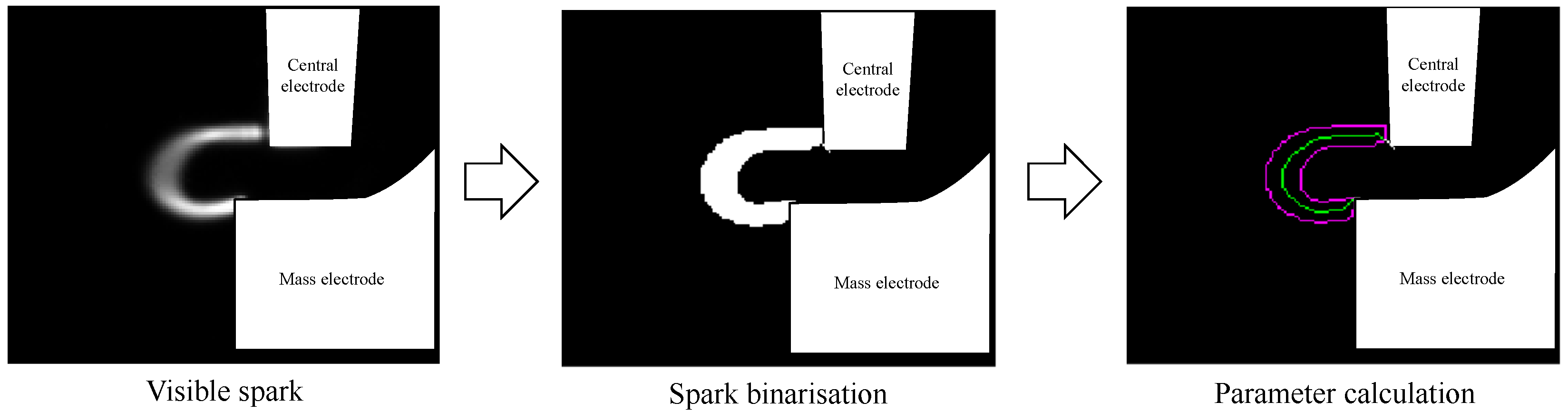
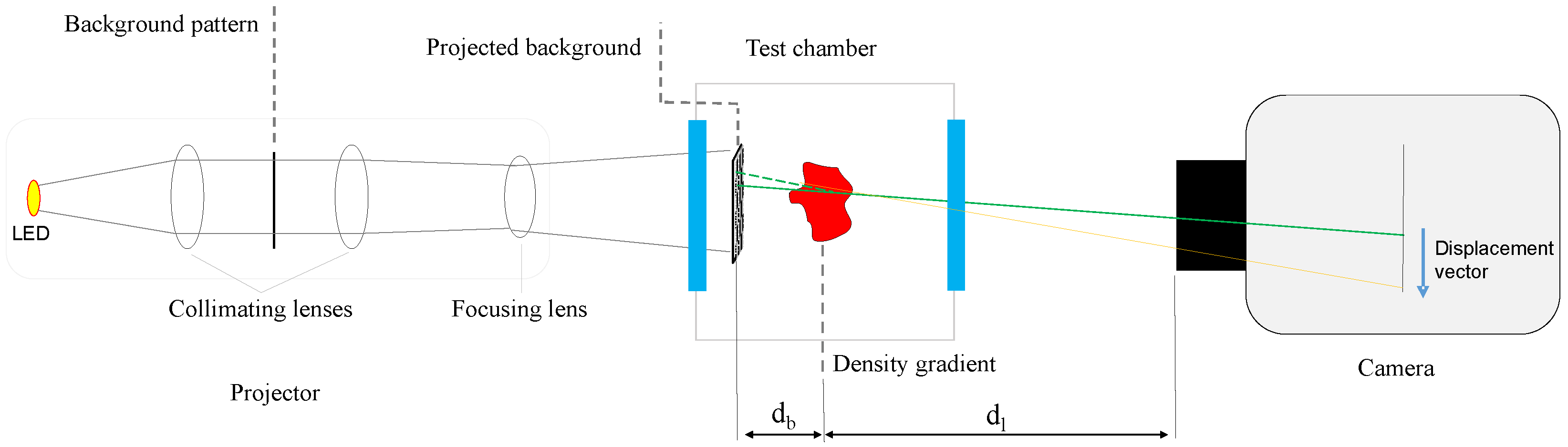
2.2. Measurement Techniques and Data Processing

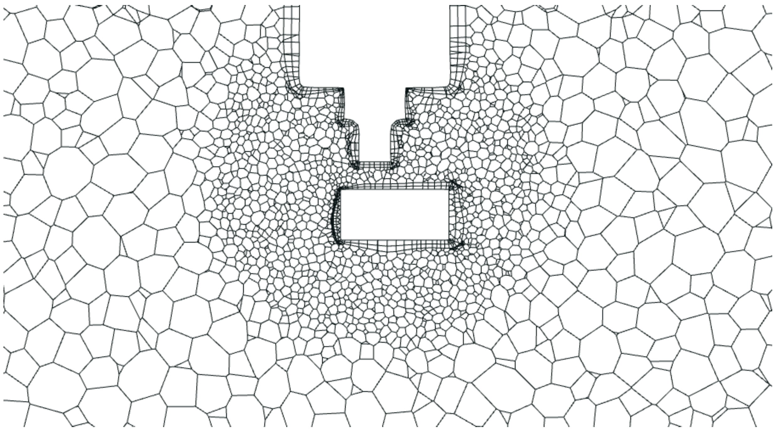
To measure the ignitable volume generated by sparks under these conditions, two different approaches were used. The first method involved detecting plasma parameters from visible plasma images captured using a high-speed camera. The second strategy involved observing the heat transfer from the plasma channel to the surrounding flow medium using Background-Oriented Schlieren (BOS).

The visible sparks were captured with f2.8 aperture and 1/119,000 s exposure time at a 100 kHz framerate with a resolution of 384 × 264 pixels and a spatial resolution of 0.035 mm per pixel. The raw images captured by the high-speed camera from the experiments were first processed to obtain only the required information. The spark was binarized with a Matlab function that uses a threshold calculated based on the local mean intensity. Then, another Matlab algorithm analyzed these binary images to obtain various parameters. In the case of visible spark observations, the algorithm detected parameters such as the length, diameter, and volume of the plasma channel. Figure 2 shows the different steps used by the algorithm to detect the plasma parameters for a spark stretched by the flow from the right.

The binarized images were also used to detect the furthermost location of the spark in these images. This information was used to calculate the tip velocity for the plasma channel.

The heat transfer from the spark was detected by Background-Oriented Schlieren (BOS) technique. The measurement principle was as follows: differences in density in a medium lead to refractive index changes that cause the passing light rays to be refracted [20]. To detect this change, two images captured using a camera were compared for small changes. One was a reference image of a background pattern, and the other was an image of the same background pattern deformed due to the refraction by the density gradient. Using algorithms capable of detecting minute changes by comparing these two images, the displacement/deformation of the background pattern was calculated. The angle of refraction could be obtained from these displacements, and from this, even the density gradient field could be calculated. Because of its simple experimental setup, this technique is commonly used to visualize and quantify density gradients [21]. However, it should be noted that the signal is integrated along the line of sight and, therefore, is significantly influenced by the thickness of the density gradient.

As per Equation (1), the displacement obtained from the BOS algorithm is directly proportional to the change in density, $\rho$ [22]. This means that the higher the change in density, the higher the deformation of the background and, therefore, the higher the displacement detected.

$$\begin{array}{cc}\hfill {\displaystyle \frac{{\partial }^2\rho (x,y)}{\partial x^2}}+{\displaystyle \frac{{\partial }^2\rho (x,y)}{\partial y^2}}& =S\left(x,y\right)\hfill \end{array}$$

(1)

In the Equation (1), the term S is derived from the displacement detected by the correlation algorithms and the experimental geometry. The measurement in this work focuses on heat transfer visualization and does not focus on temperature calculation.

The algorithm used for BOS measurements is Fast Checkerboard Demodulation (FCD). The FCD algorithm calculates the displacement vectors from the deformation of periodic background patterns [23]. This technique was selected because it offers several advantages over other techniques, such as the digital image correlation (DIC) algorithm, since it allows for faster computation while maintaining the same resolution as the raw images and does not require the consideration of additional parameters, such as interrogation windows [24]. However, the measurable range depends on the background pattern’s size, and this has to be chosen appropriately.

However, due to the high temperatures of the plasma column in a relatively small volume, sparks generate very high-density gradients. This presents a significant challenge for existing BOS techniques. Furthermore, the brief duration of the spark event (approximately 1.5 ms) presents an additional challenge in achieving high-resolution visualization. In order to achieve a high spatial resolution visualization of heat transfer from sparks, the optimal setup for a Background-Oriented Schlieren (BOS) system would involve using a background with a small periodic pattern positioned near the spark. This would ensure high spatial resolution while maintaining a low enough sensitivity for the periodic pattern to still be recognizable by the algorithms. However, there are practical limitations to consider when placing the pattern, as it may impact the flow. Additionally, due to design constraints, it is not feasible to place a physical pattern inside the test bed.

Similar studies of sparks have also been performed with laser Speckle Background-Oriented Schlieren (SBOS) [13]. However, SBOS requires a relatively complicated setup with lasers. This is also challenging to set up in the testbed where the experiments were performed. To address the aforementioned challenges, a modified BOS technique was employed. Rather than utilizing a printed background pattern situated behind the density gradient (in relation to the camera), the background was projected into the focal plane of the camera. This modified BOS technique with projected background [16,17,25] is also presented as a Forward-Projected Background-Oriented Schlieren (FPBOS) [15,18]. This is highly beneficial in this scenario as it allows the background pattern to be positioned in the desired plane within the focal range of the camera lens without disrupting the flow field. A detailed schematic of the experimental setup for the FPBOS technique is shown in Figure 3. Since this technique is extremely sensitive to the geometric setup and the pattern size used, the projector provides a flexible setup that enables both to be easily adjusted.

The measurement was performed with the same camera equipment mentioned previously. The FPBOS measurements were performed with f32 and an exposure time of 1/400,000 s captured. The images were captured at a frequency of 100 kHz with a resolution of 384 × 264 pixels (0.0304 mm/pixel). The projector consists of three achromatic lenses with a 50 mm diameter. Two are collimating lenses with a focus length of 160 mm and the third one was a focusing lens with a 147 mm focus length. A checkerboard pattern printed on an A4 plastic sheet was placed in between the collimating lenses. This pattern was illuminated by a Nichia NV4L144ART SMD-LED. The pattern was projected to a plane 7 mm behind the spark gap (i.e., d_b = 7 mm). The distance between the camera and the spark plug was 185 mm (i.e., d_l = 185 mm). Each square in the projected checkerboard had a size of approximately 0.1 mm × 0.1 mm.

Figure 4 demonstrates the results from the FPBOS measurement as well as the post-processing performed. The images also show the central and mass electrodes of the spark plug. Figure 4a shows a typical result from FPBOS measurement. The magnitude of the displacement vector field obtained from the FCD algorithm was obtained and a false colormap was applied (red—highest displacement; blue—low or zero displacement detected). It was observed that the edges of the density gradient usually had the highest displacement. The displacement vector magnitude field obtained from the FCD algorithm is integrated first as shown in Figure 4b. Here, the grayscale image is chosen for representation because of the ease of binarization. The highest value in the integrated displacement field is displayed with the greatest intensity, and the background, without any displacement, should be zero. The integrated images ertr then averaged, after which binarization (the pink region in Figure 4c) was performed to remove the background noise. The highest value appears the brightest in the integrated image. These results were then used to qualitatively validate the heat transfer from the simulation model.

3. Simulation Setup

As previously stated, a good physics-based ignition model is required to predict the spark movement and heat transfer from the spark to its surroundings. These two parameters will affect the location of the initial flame kernel formation. This section describes a Velocity Multiplier and adds a two-way coupling of the plasma particles to the standard Curved Ark Diffusion Ignition Model, which we will from here on refer to as CADIM-VM-TWP. This model attempts to overcome some deficiencies in the default Curved Arc Diffusion Ignition Model (CADIM) in AVL FIRE M R2023.2.

The spark channel is represented by discrete Lagrangian particles that are part of an evolving 3D curve [8]. The Lagrangian particles are one-way coupled to the flow field and are considered massless, and they do not have any influence on the flow field [3].

The input parameters at the ignition time consists of the secondary circuit’s initial electrical energy, E_s(0), resistance R_s, and inductance L_s. A spark initiates when the voltage reaches the breakdown voltage V_bd, a value determined by the inter-electrode distance d_ie and the gas density surrounding the spark plug, typically occurring within a few microseconds. Subsequently, in the ensuing microseconds, the gas (or, in the present model, the flame kernels) absorbs a specific amount of electrical energy E_bd, calculated as follows:

$$E_{bd}=G{\displaystyle \frac{V_{bd}^2}{C_{bd}^2·d_{ie}}}$$

(2)

where G and C_bd are constants [5,8]. The visible spark observed in experiments typically persists for several milliseconds during the main spark phase, referred to as the glow phase. Equation (3) shows the secondary current calculated in the secondary electrical circuit.

$$i_s\left(t\right)=\sqrt{{\displaystyle \frac{2E_s\left(t\right)}{L_s}}}$$

(3)

V_gc represents the voltage in the gas column along the spark length l_spk, while p denotes the gas pressure in the proximity of the spark. C_gc stands for a constant [8]. According to [26], for the spark glow mode, the value of C_gc = 40.46 yielded the best fit at atmospheric pressure and no flow. Further, d_is signifies the discharge coefficient, which defaults to −0.32.

$$V_{gc}=C_{gc}·l_{spk}·\sqrt{p}·i_s^{d_{is}}$$

(4)

The following relation determines the inter-electrode voltage V_ie, where V_cf and V_af are the drops in cathode and anode voltage [5,8,26].

$$V_{ie}\left(t\right)=V_{cf}+V_{af}+V_{gc}$$

(5)

Meanwhile, E_s, the available electrical energy on the secondary circuit, is determined by

$${\displaystyle \frac{d{E}_s\left(t\right)}{dt}}=-R_s{i}_s^2\left(t\right)-V_{ie}\left(t\right)i_s\left(t\right)$$

(6)

During the glow phase, the inter-electrode voltage V_ie may once again reach the breakdown voltage. Subsequently, another breakdown occurs, and a new spark is generated, causing the previous one to vanish. This cycle continues if there is remaining electrical energy, sustaining the glow phase.

In the ignition delay model, combustion reactions take place at the outer surface of the plasma, where conditions are ideal for rapid chemical activity (temperatures ranging from thousand to a few thousand Kelvin) [27]. This is the primary assumption for the ignition delay time sub-model. The temperature at the surface of the spark channel is determined by solving the derived 1D heat equation, taking curvature into consideration [3]. However, in this model, heat transfer is not coupled in the 3D domain because the particle is only one-way coupled to the flow field.

An ignition delay time ($\tau$) is obtained from a database for the calculated surface temperature of the spark channel and the composition of the local mixture. The instantaneous change in the ignition precursor ($d{Y}_p$) for a given ignition delay time is calculated as mentioned in Equation (7) [28].

$${\displaystyle \frac{d{Y}_p}{dt}}=\sqrt{{\displaystyle \frac{{\tau }^2+4(1-\tau )Y_p}{\tau }}}$$

(7)

The precursor value (which is initially set to zero) is calculated for each particle representing the spark. Once it reaches a value of 1.0, an initial flame kernel is formed at the location of that particle, as illustrated in Figure 5.

Once the initial flame kernel has been formed, the initial kernel growth model employs a zero-dimensional (0D) model to calculate the early growth of the flame kernel, given that this size may be too small to be resolved by the combustion model on the three-dimensional (3D) mesh.

A polyhedral mesh was employed for the simulation, as the gradient can be effectively approximated with such a mesh (due to the high density of neighboring cells). The global mesh cell size is 1 mm, with a mesh refinement near the spark plug gap (the cell size is 0.2 mm). Figure 6 depicts a cross-sectional view of the mesh.

Given that the ignition model is transient, the simulation used the transient RANS (Reynolds-Averaged Navier–Stokes equations) approach. After 0.3 s of simulation time, the flow began to converge and exhibit a steady flow pattern. The spark model was triggered after 1.5 s, which guaranteed that the flow reached a steady state.

After gaining a thorough understanding of CADIM, two major improvements were implemented to address some of the model’s shortcomings, which arise from the use of one-way coupling between the spark and the surrounding flow field. Because of the one-way coupling, the spark does not influence the flow field and moves with it. However, from experiments detailed in Section 4.2, it was discovered that the interaction between the spark and the surrounding flow field causes the spark to move at a slower velocity than the flow field. Another issue with the CADIM model is that because the coupling is one-way, the heat transfer from the spark to the surrounding environment is decoupled and cannot be observed in the 3D domain. As a result, the default CADIM model estimates the heat transfer using a 1D temperature equation, followed by a tabulated ignition delay table to check for auto-ignition caused by heat transfer. CADIM-VM-TWP includes two-way temperature coupling between the spark and its surrounding flow field using Equation (8), where Q is the rate of heat transfer from the spark to the surrounding, A is the heat transfer surface area, h_c is the convective heat transfer coefficient, and ΔT is the temperature difference between the spark and its surroundings.

$$Q=h_c·A·\Delta T$$

(8)

The empirical Equation (9) can be used to express the convective heat transfer coefficient, where V is the flow velocity [29]. Since the spark channel is modeled as Lagrangian particles, in order to calculate the area A, the diameter of each particle is equal to 0.3 mm, which is the diameter of the plasma channel [30], and the temperature is equal to 5000 K [7].

$$h_c=10.45-V+10V^{1/2}$$

(9)

CADIM-VM-TWP coupled with CFD and chemical reaction kinetics solvers allows the detection of the position and shape of the first flame kernel without the use of any tabulated ignition delay lookup tables. The chemical reaction kinetics solver calculates and detects the auto-ignition point after increasing the local heat temperature due to heat transfer from the spark, which is coupled in the new CADIM-VM-TWP ignition model with the 3D domain. This was not possible using the default CADIM ignition model.

4. Results and Discussion

This section presents and discusses the results from the experiments and simulations performed as part of this study. The comparisons are performed between the simulation results and the average experimental results.

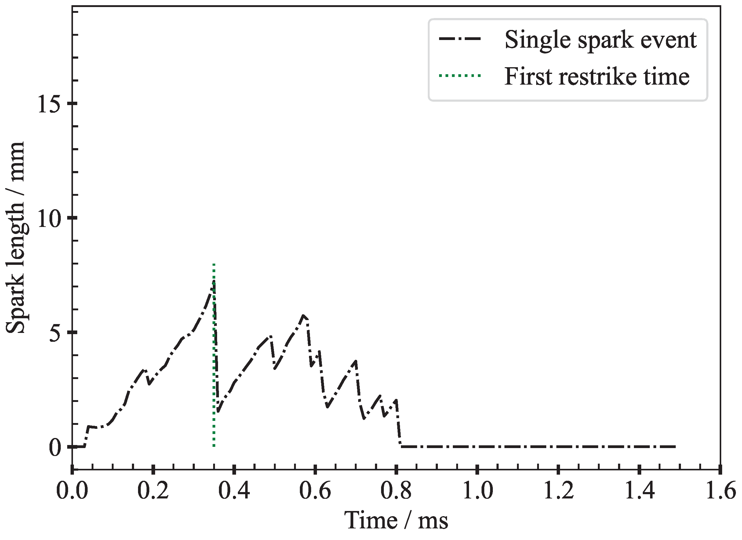
4.1. Optical Plasma Parameters

As mentioned in Section 2, a Matlab algorithm detects the spark’s optical parameters. Figure 7 and Figure 8 present the results from the algorithm to provide a clear understanding. Figure 7 shows the parameter detection in action. The images show both the raw spark images (green) and the perimeter of the spark detected by the Matlab algorithm (pink). The images also show the location of the electrodes of the spark plug (white). The algorithm does not process this region in order to avoid errors caused by the detection of glowing electrodes. The length of this plasma channel is obtained from the detected perimeter and plotted in Figure 8.

Figure 8 illustrates the variation of the spark length detected from the spark event shown in Figure 7 at a pressure of 6 bar and a flow velocity of 15 m/s, as well as the detected time of occurrence of restrikes/shortcuts. A comparison of Figure 7 and Figure 8 gives a clear idea of how the algorithm works. The time zero corresponds to the trigger. A slight delay of approx. 0.4 ms was observed between the trigger and the plasma channel formation (breakdown). The image captured by the camera immediately after the breakdown is not used for processing because it is very bright and results in an overexposed image. Row ’a’ in Figure 7 shows the elongation of the plasma channel due to the flow from the right. This can be seen clearly with the continuous length increase between 0.5 ms to 0.15 ms in Figure 8. At a time of 0.19 ms after the breakdown, a shortening of the length is seen in Figure 8. This is a shortcut, which is when the plasma channel intersects with itself, shortening its length, as seen in the frame 0.19 ms after the trigger in row ’b’ in Figure 7. Another significant change in the length is seen at 0.36 ms, and this is due to the occurrence of a restrike. This is when an existing plasma channel ceases to exist and a new plasma channel is formed between the electrodes seen clearly in frame 0.36 ms, row ’c’, in Figure 7. These show that at the time of occurrence of these phenomena, a slight overestimation of the length occurs due to the algorithm detecting the old and new plasma channels.

To obtain statistically representative information about the average spark, 100 spark events were captured. Figure 9 shows the average length of 100 spark events at 6 bar pressure and 15 m/s flow velocity detected by the algorithm, as well as the mean and standard deviation of the time of occurrence of the first restrike/shortcut. The time of occurrence of the first restrikes from these plots was detected based on the prominence of the peak (a minimum prominence of 1 mm was used as the criterion) by using the Matlab function ’Findpeaks’. Prominence is a measure of how much a peak stands out in comparison to the other peaks in the plot.

However, it can be seen that the arithmetic average length of the 100 sparks at each timestep does not represent the true spark behavior. This is because restrikes or shortcuts cannot be observed in the averaged spark length, unlike in the individual sparks, and the spark length appears to decrease when the location of restrikes and shortcuts varies significantly. This can be seen in Figure 9, which shows a decrease in the average spark length following the average time of occurrence of the first restrike/shortcut. Therefore, the average length from the spark until the average time of occurrence of the first restrike/shortcut was considered relevant for this study.

4.2. Velocity Multiplication Factor—Incorporation and Calibration

To evaluate the ignition simulation model, the volume that can ignite the mixture was considered as the important parameter. Since the original CADIM did not have two-way-coupled particles, the length of the plasma channel was taken as the criterion for evaluation. Figure 10 shows the non-calibrated simulation performed at 6 bar of absolute pressure and 15 m/s average flow velocity. It was seen that the spark in the simulation was activated immediately at the trigger. However, a delay was observed in the test bench, and the breakdown occurred approximately 0.04 ms after the trigger. The start of ignition in the simulation is therefore delayed by 0.03 ms to take this phenomenon into account. More crucially, the plasma was stretched more rapidly in the simulation, and the restrike occurred earlier than seen in the experimental case. This has to be due to the relation of the flow field velocity to the simulated spark velocity.

As a first step in understanding this flow–spark interaction, the velocity of the plasma channel was inspected. In the simulation model, the plasma channel particles had the same velocity as the surrounding flow field. From the experiments, the velocity of the tip (the point furthest from the spark gap) of the spark was obtained as shown in Figure 11. As the velocity in the flow direction is considered to be the dominant component influencing the elongation of the spark, only this component is taken for comparison. This approach also simplifies the validation process. Furthermore, only the tip of the spark is considered for velocity evaluation, as this is the location that is influenced the most by the flow.

Figure 11 shows the velocity of the simulated and experimental spark tip obtained. The experimental results are obtained by the Matlab script described in Section 2. The plotted experimental result is averaged over 100 spark event measurements. The velocities were only taken till 0.28 ms after the trigger because the occurrence of restrikes started to influence the average velocities significantly. When taking only the experimental results into account, it can be seen that the velocity of the spark tip is the highest at the beginning; i.e., in the spark gap. When compared to the average flow velocity of 15 m/s, this measured average spark tip velocity varied by a factor of approximately 0.87 right after the breakdown, which later decreased to about 0.51 when the spark tip was further away from the spark gap. However, these results cannot be directly compared because the flow is not uniform everywhere, as can be seen from the simulated flow field shown in Figure 12.

Figure 12 shows the resultant flow field including the flow direction. The flow goes from the right to the left at a velocity of 15 m/s at an absolute pressure of 6 bar. The flow is accelerated in the spark gap up to a maximum of 24 m/s, and the velocity is higher near the mass electrode than the central electrode. The flow is obstructed by the electrodes, and the flow gets slower behind the sparkplug, leading to the formation of stagnation zones. This result shows that the spark should have the highest velocity in the electrode gap. This should decrease immediately as the spark exits the gap and the farther the spark tip is from the electrodes, the more likely it is to reach the bulk flow velocity. However, from the results shown in Figure 11, the velocity at each point is lower than the flow field velocity. This could be because the spark in between the electrodes offers a higher resistance to the flow as a result of the denser electromagnetic field here. This becomes weaker the farther the spark is from the electrodes.

Since the simulated plasma channel in CADIM has the same velocity as the local flow, the tip velocity of this plasma channel was detected for each timestep manually and is shown in Figure 12. The average experimental results (100 events) are also plotted in this figure, and it can be seen that they follow a similar trend even though the velocities are significantly different. The velocities of the experimental results are different from those of the simulation results by a factor of approximately 0.6 at each time step. To take this effect into account and simplify the calibration of the simulation model, a velocity multiplication factor (VM) was integrated into CADIM. Using this VM, the velocity of the particles that form the spark will be adjusted based on the flow field velocity of the adjacent mesh cells.

Using the information obtained from these tests, the VM value was calibrated for the optimum match with experimental results. Since the metric for the model evaluation remains the length of the plasma channel, the simulation plasma channel length was compared to the experimental results. With a value of 0.675, both the spark length and the location of the first restrike from the simulation results were extremely close to the experimental results, as depicted in Figure 13. This is an encouraging sign that the experimental results produced a quantifiable improvement in the simulation model. It is important to note that the results are only compared until the first restrike.

Using the newly calibrated VM, the spark tip velocity was once again calculated, as shown in Figure 14. Here, the results from the modified simulation model (continuous red line) show significant improvement to the earlier simulation model, and this is also encouraging. It still has a slightly different velocity from the experimental results. However, this could be due to the fact that the model is calibrated on the basis of the length of the plasma channel.

Since a good agreement was achieved with a VM of 0.675, the simulated spark and the average spark obtained from the experimental results were compared. Figure 15 compares the average spark from 100 spark events in the bottom row and the simulated spark in the top row at different time steps at a pressure of 6 bar and a flow velocity of 15 m/s. The first set of images is from 0.01 ms after the breakdown (0.05 ms after the trigger), and the rest are at 0.05 ms intervals. This step aims to understand if the simulated spark behaves similarly to the experimental case. The images were processed to have a similar scale to facilitate this qualitative comparison. From these images, it can be seen that the spark produced by CADIM-VM lies within the possibilities observed in the experiments. However, the shapes are slightly different even though the lengths remain similar, as mentioned in the previous comparison shown in Figure 13. It can be seen that the experimental spark is stretched a little further near the mass electrode than near the central electrode (downward stretching). The simulated spark is stretched more symmetrically and the spark tip lies in a plane in between the electrode gaps. Further, the experimental spark follows a more complicated path, and the root travels along the electrode depending on the flow, in contrast to the simulated spark, which travels only along the horizontal surface of the electrodes. This movement also shows significant cycle-to-cycle variation in the experiments. The difference in the shape of the simulated spark can be attributed to this difference and presents a further topic for the improvement of the simulation model. Nonetheless, the results still show significant improvement with the incorporation of the VM since the spark stretching and the location of the sparks seem to not be significantly different from each other.

To further inspect the performance of the modified simulation model with the calibrated VM, a variation in pressure and flow velocity was carried out. Figure 16 shows the comparison of results for a pressure of 11 bar with the same flow velocity of 15 m/s. Once again, without the velocity modification, the simulation indicated a trend toward higher spark stretching velocities than the experimental data, which was consistent with previous results. However, utilizing the same value of the VM resulted in an improvement in the simulation results despite its calibration at a different pressure of 11 bar. This underscores the robustness of the value of the VM used. It can be seen that in the simulation, the first restrike occurred earlier than that in the experiment. However, it occurred at 0.33 ms in the calibrated simulation, which is within the range of standard deviation in the experimental results (0.37 ± 0.06 ms).

As a further step, a velocity variation was performed with an average flow velocity of 10 m/s and an absolute pressure of 6 bar. Figure 17 shows a plot similar to the previous results. Once again, the use of a VM value of 0.675 resulted in an improvement in the simulation results. This can be seen from the similar slopes of the experimental and simulation results. The slope shows the rate of change in the length of the plasma channel, and this means that the simulation shows the same rate of plasma channel elongation as the experimental results. However, the simulated spark (both with and without VM) reaches the restrike early and outside the range of standard deviation of the time of occurrence of the first restrike in the experiments. The reason for this is that in the experiment, the mean first restrike occurred later than in the previous conditions. However, in the simulation model, the energy is insufficient to maintain the spark until that point. Therefore, the energy in the electrical circuit must also be calibrated.

Incorporating the Velocity Multiplier factor (VM) calibrated for one operational condition improved the performance of the simulation model for other conditions. Additionally, calibrating the VM and other parameters, such as energy, for each specific test condition can lead to even better simulation results providing a possibility for a database-driven model.

4.3. Heat Transfer by 2-Way Coupling of Plasma Particles in CADIM

As mentioned in Section 3, the two-way coupling of plasma particles was also carried out in the CADIM by means of a user-defined function. This modified model, the CADIM-VM-TWP, along with the calibrated Velocity Multiplier, is further evaluated by comparing it with the FPBOS experimental results. The volume of the medium heated by the spark in the simulation is extracted as an iso-volume of over 300 K. Since the FPBOS measurement detects any changes in the density in the observation field, it is comparable to the iso-volume projection in the simulation. In order to understand the heat transfer results from the simulation, these iso-volume projections were compared to the heated volume detected by the BOS experiments.

Figure 18 shows the comparison of the CADIM-VM-TWP and the heat transfer detected by the FPBOS technique. The first images immediately follow the breakdown, and the following images are 0.05 ms from each other. The simulation results show a projection of the 300 K iso-volume. The experimental results show averaged heated volume projection obtained from FPBOS measurement of 10 spark events. The displacement vectors obtained from FPBOS results were integrated, averaged, and segmented, as described in Section 2. In Figure 18, noting that the size of the spark gap is 0.7 mm, it can be seen that the density gradients generated by the spark can be visualized at high spatial resolution (pixel = 0.0304 mm ). Under these experimental conditions, it was not possible to obtain high-resolution visualization from previously existing BOS techniques.

The initial observation was that the heated volume in Figure 18 is significantly larger than the plasma channel shown in Figure 15. This is true in both the simulated and the experimental cases. Since the goal was to obtain good agreement with the physical phenomenon of the spark, i.e., the heat transfer followed by inflammation, this is certainly a step in the right direction.

Upon comparing the results shown in Figure 18, it can be seen that the simulation results differ in some respects from the experimental results. The projected area and the location of the heated volume look similar in both cases. However, following the breakdown, it was seen that the heated volume travels faster in the experiments (as seen at timestep 0.06 ms). This is the effect of the breakdown that induces a sudden acceleration downstream of the flow. The simulation results do not show this. This phenomenon is more pronounced right after the breakdown and this signal dissipates with time.

It can also be seen that the simulation results show that the heated volume develops along the horizontal axis. In other words, the heat is spread symmetrically about a horizontal plane along the middle of the spark gap. In the experiments, this heat transfer is not symmetric. There is a downward movement of the heated medium with more heated volume behind the electrodes. This is similar to the movement of the plasma channel (simulated as well as experimental) that was observed in Figure 15. This could be due to the flow being slower behind the electrodes. In the simulation, the heat seems to originate from the edges of the electrode where the plasma roots are. This shows the absence of heat transfer from the electrodes in the simulation.

The results show that CADIM-VM-TWP shows improved results from the tests, especially considering that the heat transfer was absent in the previous model. The heated volume looks similar to the results obtained from the experiments. Further, the FPBOS measurement technique provides far more information regarding the spark phenomenon than the observation of just the visible spark.

5. Conclusions

The aim of this work was to gain a deeper understanding of the spark ignition phenomenon and utilize the gained information to improve the simulation models. The optical measurement techniques presented in this work provided not only qualitative but also quantitative information regarding the spark ignition phenomenon. This helped in improving the ignition simulation model to accurately represent the physical phenomenon, which is required to accelerate the development of innovative technologies to optimize internal combustion engines using renewable fuels like hydrogen and methanol with advanced ignition systems like prechambers.

The visible plasma channel detected using a high-speed camera was used to obtain the temporal evolution of spark length using Matlab scripts. The initial observation of the spark velocity led to the incorporation of a Velocity Multiplier (VM) to address the observed difference in plasma and flow velocities. The results mentioned in this work were performed with a focus on the experimental conditions of 6 bar and 15 m/s. This VM was calibrated to match the simulated plasma channel length to the experimental spark length. An excellent match was obtained with a VM value of 0.675. Using this VM value also resulted in an improvement in the performance of the model for other experimental conditions as well. This shows the promise of the approach detailed here, opening up the possibility of a data-driven model from VM calibrated for different measurement conditions, improving the simulation results.

The volume heated by the spark was also observed using a modified Background-Oriented Schlieren (BOS) technique with the projected background, also known as Forward Projected Background-Oriented Schlieren (FPBOS). This, in combination with Fast Checkerboard Demodulation (FCD), provided a high-spatial-resolution visualization of density gradients generated by sparks in engine conditions. The information gained from the results was used to improve the CADIM model by incorporating heat transfer from the plasma particles to the surrounding medium. The heated volume obtained from the simulation was compared to the experimental results. The comparison showed good agreement. The improved ignition simulation model, CADIM-VM-TWP, therefore provides a better physical representation of the ignition phenomenon.

References

1. Schumacher, M.; Russwurm, T.; Wensing, M. Pre-Chamber Ignition System for Homogeneous Lean Combustion Processes with Active Fuelling by Volatile Fuel Components; Expert-Verlag: Berlin, Germany, 2018. [Google Scholar] [CrossRef]
2. Zhu, S.; Akehurst, S.; Lewis, A.; Yuan, H. A review of the pre-chamber ignition system applied on future low-carbon spark ignition engines. Renew. Sustain. Energy Rev. 2022, 154, 111872. [Google Scholar] [CrossRef]
3. Schaefer, L. Modeling and Simulation of Spark Ignition in Turbocharged Direct Injection Spark Ignition Engines; Verlag Dr.Hut: Munich, Germany, 2016. [Google Scholar]
4. Tan, Z.; Reitz, R.D. An ignition and combustion model based on the level-set method for spark ignition engine multidimensional modeling. Combust. Flame 2006, 145, 1–15. [Google Scholar] [CrossRef]
5. Duclos, J.; Colin, O. Arc and Kernel Tracking Ignition Model for 3D Spark-Ignition Engine Calculations. In Proceedings of the The Fifth International Symposium on Diagnostics and Modeling of Combustion in Internal Combustion Engines (COMODIA 2001), Nagoya, Japan, 1–4 July 2001; pp. 343–350. [Google Scholar]
6. Dahms, R.; Fansler, T.; Drake, M.; Kuo, T.W.; Lippert, A.; Peters, N. Modeling ignition phenomena in spray-guided spark-ignited engines. Proc. Combust. Inst. 2009, 32, 2743–2750. [Google Scholar] [CrossRef]
7. Kim, J.; Scarcelli, R.; Karpatne, A.; Subramaniam, V.; Breden, D.; Raja, L.L.; Zhai, J.; Lee, S.Y. Numerical investigation of the spark discharge process in a crossflow. J. Phys. D Appl. Phys. 2022, 55, 495502. [Google Scholar] [CrossRef]
8. AVL List GmbH. FIRE™ M User Manual: R2023.2; AVL List GmbH: Graz, Austria, 2023. [Google Scholar]
9. Schneider, A.; Leick, P.; Hettinger, A.; Rottengruber, H. Experimental Studies on Spark Stability in an Optical Combustion Vessel under Flowing Conditions; Springer Vieweg: Wiesbaden, Germany, 2016. [Google Scholar] [CrossRef]
10. Kim, W.; Bae, C.; Michler, T.; Toedter, O.; Koch, T. Spatio-Temporally Resolved Emission Spectroscopy of Inductive Spark Ignition in Atmospheric Air Condition; Expert-Verlag: Berlin, Germany, 2018. [Google Scholar] [CrossRef]
11. Michler, T.; Toedter, O.; Koch, T. Measurement of temporal and spatial resolved rotational temperature in ignition sparks at atmospheric pressure. Automot. Engine Technol. 2020, 5, 57–70. [Google Scholar] [CrossRef]
12. Verhoeven, D. Interferometric spark calorimetry. Exp. Fluids 2000, 28, 86–92. [Google Scholar] [CrossRef]
13. Michalski, Q.; Benito Parejo, C.J.; Claverie, A.; Sotton, J.; Bellenoue, M. An application of Speckle-based Background-Oriented Schlieren for optical calorimetry. Exp. Therm. Fluid Sci. 2018, 91, 470–478. [Google Scholar] [CrossRef]
14. Grüninger, M.; Toedter, O.; Koch, T. Optical Analysis of Ignition Sparks and Inflammation Using Background-Oriented Schlieren Technique. Energies 2024, 17, 1274. [Google Scholar] [CrossRef]
15. Kottakalam, S.; Rottenkolber, G.; Trapp, C. Forward projected Background-Oriented Schlieren for study of sparks in internal combustion engines. In Proceedings of the International Symposium on the Application of Laser and Imaging Techniques to Fluid Mechanics, Lisbon, Portugal, 8–11 July 2024; pp. 1–16. [Google Scholar] [CrossRef]
16. Leopold, F.; Jagusinski, F.; Demeautis, C.; Ota, M.; Klatt, D. Increase of Accuray for Cbos by Background Projection. In Proceedings of the 15th International Symposium on Flow Visualization, Minsk, Belarus, 25–28 June 2012. [Google Scholar]
17. Sugisaki, H.; Lee, C.; Ozawa, Y.; Nakai, K.; Saito, Y.; Nonomura, T.; Asai, K.; Matsuda, Y. Single-pixel correlation applied to Background-Oriented Schlieren measurement. Exp. Fluids 2022, 63, 36. [Google Scholar] [CrossRef]
18. Kottakalam, S.; Alkezbari, A.; Rottenkolber, G.; Trapp, C. Developing Optical measurement techniques for improving ignition simulation models. In Proceedings of the 14th International ERCOFTAC Symposium on Engineering Turbulence Modelling and Measurements, Barcelona, Spain, 6–8 September 2023. [Google Scholar]
19. Maly, R. Spark Ignition: Its Physics and Effect on the Internal Combustion Engine. In Fuel Economy in Road Vehicles Powered by Spark Ignition Engines; Plenum Press: Boston, MA, USA, 1984; pp. 91–148. [Google Scholar] [CrossRef]
20. Dalziel, S.; Hughes, G.; Sutherland, B. Whole-field density measurements by ‘synthetic Schlieren’. Exp. Fluids 2000, 28, 322–335. [Google Scholar] [CrossRef]
21. Raffel, M. Background-Oriented Schlieren (BOS) Techniques. Exp. Fluids 2015, 56, 60. [Google Scholar]
22. Venkatakrishnan, L.; Meier, G. Density Measurements Using the Background-Oriented Schlieren Technique. Exp. Fluids 2004, 37, 237–247. [Google Scholar] [CrossRef]
23. Wildeman, S. Real-time quantitative Schlieren imaging by fast Fourier demodulation of a checkered backdrop. Exp. Fluids 2018, 59, 97. [Google Scholar] [CrossRef]
24. Shimazaki, T.; Ichihara, S.; Tagawa, Y. Background-Oriented Schlieren technique with fast Fourier demodulation for measuring large density-gradient fields of fluids. Exp. Therm. Fluid Sci. 2022, 134, 110598. [Google Scholar] [CrossRef]
25. Yamagishi, M.; Ichihara, S.; Tagawa, Y.; Ota, M. Small-Scale BOS Measurement Using Background Projection. In Proceedings of the International Symposium on the Application of Laser and Imaging Techniques to Fluid Mechanics, Lisbon, Portugal, 8–11 July 2024; pp. 1–11. [Google Scholar] [CrossRef]
26. Kim, J.; Anderson, R.W. Spark Anemometry of Bulk Gas Velocity at the Plug Gap of a Firing Engine. SAE Trans. 1995, 104, 2256–2266. [Google Scholar]
27. Heywood, J.B. Internal Combustion Engine Fundamentals, 2nd ed.; McGrawHill Book Company: New York, NY, USA, 1988. [Google Scholar]
28. Francois, L.; Castagne, M.; Dumas, J.; Henriot, S. Development and Validation of a Knock Model in Spark Ignition Engines Using a CFD Code; SAE International: Warrendale PA, USA, 2002. [Google Scholar] [CrossRef]
29. Khabari, A.; Zenouzi, M.; O’Connor, T.; Rodas, A. Natural and Forced Convective Heat Transfer Analysis of Nanostructured Surface. Lect. Notes Eng. Comput. Sci. 2014, 1, 317–319. [Google Scholar]
30. Tambasco, C.; Li, D.; Hall, M.; Matthews, R. Spark Ignition Discharge Characteristics under Quiescent Conditions and with Convective Flows; SAE International: Warrendale PA, USA, 2021. [Google Scholar] [CrossRef]
Figure 1. The spark windtunnel testbed: (a) Top view (schematic). (b) View from the camera.
Energies 17 04640 g001
Figure 2. The processing steps used by the Matlab algorithm.
Energies 17 04640 g002
Figure 3. The experimental setup for FPBOS.
Energies 17 04640 g003
Figure 4. Heat transfer visualization with FPBOS and post-processing. (a) Displacement vector magnitude with an applied false color map. (b) Normalized grayscale image of the Integrated displacement vectors. (c) Projected density gradient detected by the algorithm shown in pink (conditions: 6 bar, 15 m/s, 0.06 ms after breakdown).
Energies 17 04640 g004
Figure 5. Illustration of two consecutive time steps showing the spark precursor and the subsequent development of an initial flame kernel (red sphere).
Energies 17 04640 g005
Figure 6. A cross-sectional view of the CFD mesh, with the central and mass electrodes clearly visible.
Energies 17 04640 g006
Figure 7. Spark parameter detection by the algorithm for a single spark event. The image series shows the following phenomena: (a) spark elongation, (b) shortcut, and (c) restrike (test conditions: 6 bar pressure and 15 m/s flow velocity).
Energies 17 04640 g007
Figure 8. Spark length and first restrike detected by the algorithm for a single spark event (test conditions: 6 bar pressure and 15 m/s flow velocity).
Energies 17 04640 g008
Figure 9. Mean spark length (100 spark events) obtained using the Matlab algorithm with the mean and standard deviation of the time of the occurrence of the first restrike (test conditions: absolute pressure = 6 bar, flow velocity = 15 m/s).
Energies 17 04640 g009
Figure 10. Simulated spark length (CADIM) compared to the experimental data (averaged over 100 cycles) till the first restrike (test conditions: absolute pressure = 6 bar, flow velocity = 15 m/s).
Energies 17 04640 g010
Figure 11. Spark tip velocity from the simulated and experimental (averaged over 100 events) results (test conditions: absolute pressure = 6 bar, flow velocity = 15 m/s).
Energies 17 04640 g011
Figure 12. Velocity flow field in a cross-section along the middle of the electrodes (test conditions: absolute pressure = 6 bar, flow velocity = 15 m/s).
Energies 17 04640 g012
Figure 13. The simulated spark length compared to the averaged experimental data (100 events) till the first restrike location (test conditions: absolute pressure = 6 bar, flow velocity = 15 m/s).
Energies 17 04640 g013
Figure 14. Simulated spark tip velocity compared to the average experimental data (100 events) (test conditions: absolute pressure = 6 bar, flow velocity = 15 m/s).
Energies 17 04640 g014
Figure 15. Spark shape comparison of the simulated (VM = 0.675) and average experimental (bottom row) results (100 events) (test conditions: absolute pressure = 6 bar, flow velocity = 15 m/s).
Energies 17 04640 g015
Figure 16. Simulated spark length compared to the average experimental data (100 events) till the first restrike location (test conditions: absolute pressure = 11 bar, flow velocity = 15 m/s).
Energies 17 04640 g016
Figure 17. Simulated spark length compared to the averaged experimental data (100 events) till the first restrike (test conditions: absolute pressure = 6 bar, flow velocity = 10 m/s).
Energies 17 04640 g017
Figure 18. Heat transfer from the spark: comparison of average experimental results (10 events) and the 300 K iso-volume projections obtained from the CADIM-VM-TWP simulation (test conditions: absolute pressure = 6 bar, flow velocity = 15 m/s).
Energies 17 04640 g018