Abstract
In response to global energy, environment, and climate concerns, distributed photovoltaic (PV) power generation has seen rapid growth. However, the intermittent and uncertain nature of PVs can cause voltage fluctuations in distribution systems, threatening their stability. To address this challenge, this paper proposes an active distribution network voltage optimization method, of which the main contribution is the development of a comprehensive voltage optimization strategy that integrates day-ahead prediction and real-time adjustment, significantly enhancing the stability and efficiency of distribution networks with high PV penetration. In the day-ahead prediction stage, the forecast scenarios of load and PV output guide network reconfiguration for improved voltage distribution. In the real-time operation stage, flexible regulation of PV and energy storage systems is used to adjust power outputs, further optimizing voltage quality. Simulations on the IEEE 33-bus system show that the method effectively improves voltage distribution, enhances renewable energy consumption, and ensures the safe, economic operation of the distribution system.
1. Introduction
As global concerns about energy, the environment, and climate issues escalate, the advancement of clean and renewable energy sources, including wind power and photovoltaic (PV) energy, has emerged as a crucial endeavor across numerous countries [1]. In this context, distributed PV power generation and other related technologies have experienced rapid development. However, compared with traditional thermal power and hydropower, etc., PV power generation is characterized by intermittency, stochasticity, and uncertainty [2]. Because of the unpredictable nature of load demand and renewable energy sources like PV power generation, it may lead to intermittent voltage violations and other problems in the distribution system, which significantly affects its safe operation [3,4]. Therefore, studying the voltage optimization problem within distribution systems with high penetration of PV energy is of utmost importance.
In view of the above problems, the traditional voltage regulation method has certain defects. For example, transformer tap switch regulation and capacitor regulation are discrete voltage regulation methods [5], which have high operating costs and cannot be operated frequently. Compared with the traditional voltage regulation methods, the inverter of the PV power generation system has a preset redundant capacity, which can be used for reactive power regulation more quickly and flexibly [6]. At the same time, the energy storage system (ESS) is connected to the distribution grid through an inverter device, which has the ability of fast and flexible regulation in four quadrants [7]. Therefore, more flexible and fast voltage regulation can be realized by utilizing the PV power generation system and ESS, which has prompted extensive research. Ref. [8] mitigates the violation of voltage by adjusting the output of the PV inverter, realizing voltage regulation through operation modes such as preventive control, emergency control, and restoration control. Ref. [9] proposes a short-term ESS for improving the voltage quality problem in distributed wind power systems. Ref. [10] proposes a distributed control strategy for coordinating multiple ESSs for voltage regulation in active distribution networks with high penetration of fluctuating renewable energy sources. Ref. [11] investigates a method to improve voltage quality in low-voltage distribution networks by utilizing the reactive power capability of single-phase PV inverters.
With the development of active distribution network technology, new technical means have emerged for voltage control in the distribution network, and flexible distribution network reconfiguration can effectively improve the voltage distribution. For example, Ref. [12] establishes a two-stage optimization model to reduce the impact of PV power generation on voltage by reducing the equivalent impedance of the Davignan model at the common connection point through distribution network reconfiguration. Ref. [13] proposes a mixed-integer programming model for the reconfiguration of active distribution systems that considers voltage dependency, the type of loads, and renewable sources. Ref. [14] achieves preventive voltage control in distribution networks by reconfiguring the network. This approach addresses voltage security issues and ensures the safe operation of distribution networks. Ref. [15] improves voltage distribution within the distribution network by coordinating the regulation of both active and reactive power of distributed generations (DGs). Ref. [16] proposes coordinating the operation of multiple voltage regulators and DGs in the distribution system to achieve effective voltage control under changes in network structure and DG availability.
Utilizing the flexibility of multiple source-network-load-storage resources of the distribution network, and considering the coordination of the above resources, the voltage optimization of the distribution network can be realized more effectively [17,18]. For example, Ref. [19] proposes a real-time voltage regulation strategy for reconfigurable low-voltage distribution networks. By coordinating the optimal feedforward control of DGs with the operation of line switches, pre-compensation of impending voltage deviations during network reconfiguration-assisted load restoration is achieved. Ref. [20] explores techniques for managing voltage fluctuations in low-voltage distribution systems with a significant presence of PV penetration. Where, a wide range of applications of three types of flexible resources, namely source, network, and storage, are considered for voltage regulation of low-voltage distribution networks. Ref. [21] considers the coordination of electric vehicles and PVs to achieve voltage optimization in distribution networks with active network losses and voltage fluctuations as optimization objectives. Ref. [22] achieves distribution network voltage quality optimization through dynamic reconfiguration of the distribution network in concert with energy storage and other synergies. Ref. [23] presents a control framework based on source-grid-load collaboration to enhance power quality in distribution networks with high penetration of low-carbon energy sources. Ref. [24] proposes optimal locations for distributed PV generation to identify and mitigate voltage limit violations.
Although many relevant studies have been carried out on the voltage optimization problem of distribution networks under high PV penetration, existing studies have not simultaneously considered the coordination of PV generation systems, network reconfiguration, load demand, and ESS in different time scales. So, achieving efficient utilization of renewable energy and ensuring the economic operation of the grid becomes challenging. Therefore, this paper proposes an active distribution network voltage optimization method based on the coordination and interaction of source-network-load-storage resources. Where, in the day-ahead prediction stage, based on the forecasted scenarios of PV generation and load demand, the reconfiguration scheme for the distribution network is formulated, and the voltage distribution is improved by optimizing the topology of the network. In the real-time operational phase, taking into account the variability of load demand and PV generation across different scenarios, the flexibility of PV inverters and ESSs is harnessed to make instantaneous adjustments. The active and reactive power outputs of the PV generation systems, as well as the charging and discharging power of the ESSs, are fine-tuned in real-time. This dynamic adaptation is implemented according to the differing scenarios of load demands and PV outputs. Consequently, the voltage quality of the distribution network is further enhanced, and the capacity to utilize renewable energy is effectively increased.
The main contributions of this paper are summarized as:
- (1)
- An active distribution network voltage optimization method based on source-network-load-storage coordination and interaction is proposed.
The method leverages the flexibility of PV generation systems, ESSs, load demand, and network reconfiguration to optimize the voltage quality of distribution networks. By formulating a distribution network reconfiguration plan in the day-ahead prediction stage and adjusting the active and reactive power outputs of PV systems and charging/discharging powers of ESSs in real-time, the method effectively improves voltage distribution and ensures safe and economic operation.
- (2)
- A 0–1 mixed-integer second-order cone programming model based on the scenario-based stochastic optimization for voltage optimization is established.
Taking into account the uncertainties associated with PV output and load demand, a scenario-based stochastic optimization model is devised to optimize voltage levels. This model encompasses network topology constraints, power flow and security constraints, load demand constraints, PV generation system operational constraints, and ESS operational constraints, among others. Structured as a 0–1 mixed-integer second-order cone programming problem, this model offers enhanced extensibility, making it easier to incorporate additional voltage regulation measures in the future.
- (3)
- The scenario decomposition algorithm is introduced as an efficient solution.
To tackle the complexity of the large-scale stochastic optimization problem, an efficient solution algorithm based on the scenario decomposition algorithm is employed. This algorithm decomposes the original large-scale problem into multiple smaller, independent subproblems, each considering a single scenario. This provides potential for parallel computing on multiple computers.
The rest of the paper is organized as follows: Section 2 describes the model framework and the formulation of the proposed model; Section 3 elaborates on the model solution method; Section 4 verifies the effectiveness of the model using the IEEE 33-node distribution system; and Section 5 summarizes this paper.
2. Model Formulation
Considering the uncertainty of PV generation and load demand, this paper employs a scenario-based stochastic optimization approach to develop the voltage optimization model. The structural framework is depicted in Figure 1.
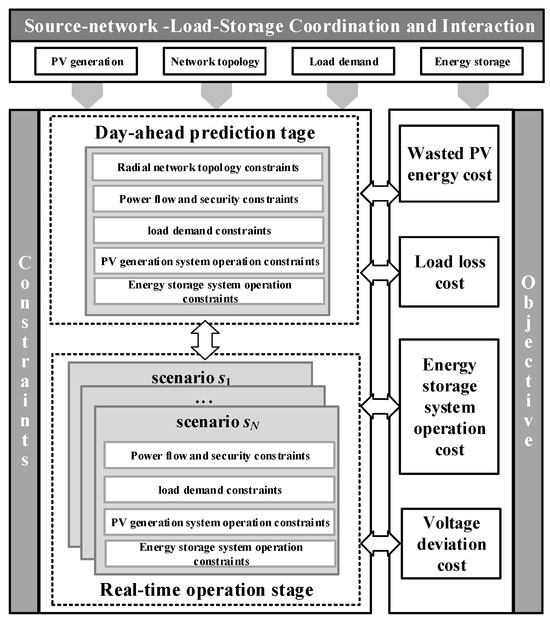
Figure 1.
Framework of the proposed model.
2.1. Day-Ahead Prediction Stage Constraints
The day-ahead prediction stage constraints contain radial network topology constraints, power flow and security constraints, load demand constraints, PV generation system operation constraints, and ESS operation constraints.
Distribution networks are usually closed-loop designed and open-loop operated with a radial topology [25]. Therefore, the radial network topology constraints are shown as constraints (1)–(3) [26].
where, constraint (1) represents the virtual flow injection constraint of the nodes in the previous day stage. Constraint (2) represents the limitation constraint of the lines flowing through the virtual flow. Constraint (3) represents the coupling constraint between the total number of closed lines and root nodes. M is a large number used for mathematical modeling purposes. is a binary variable indicating whether node i is the root node of the islanded network ( if yes, and if no). is a binary variable indicating whether line l is closed ( if yes, and if no). represents the virtual flow flowing through line l in the day-ahead prediction stage. is the set of distribution lines. is the set of nodes. is the total number of nodes in the network.
The power flow and security constraints for the day-ahead prediction stage are represented as constraints (4)–(10).
where, constraints (4) and (5) represent the balance constraints for active and reactive power injections, respectively. Constraints (6) and (7) are derived from the power flow equation, which is based on the linearized DistFlow model [26]. Constraints (8) and (9) are the active and reactive power capacity constraints of the lines, respectively. Constraint (10) is the upper and lower voltage limit constraints at the nodes. and are the active and reactive load demands at node i at time t, respectively. and are the actual active and reactive outputs of the PV system at node i at time t. and are the charging and discharging powers of the ESS at node i at time t. is the reactive outputs of the energy storage inverter. and are the active and reactive losses of the active and reactive loads of node i at time t. and are the active and reactive power flow of line l at time t. is the set of lines which are connected to node i. is the voltage of node i at time t. and are the resistance and reactance of line l, respectively. is the reference voltage. is the set of nodes at the two ends of line l; is the set of time periods considered at the day-ahead prediction stage. and are the active and reactive power flows of line l. and are the voltage limits.
The load demand constraints for the day-ahead prediction stage are expressed as constraints (11)–(12).
where, constraint (11) and constraint (12) are the active and reactive load demand constraints for the day-ahead prediction stage, respectively.
In order to fully utilize renewable energy sources, the inverters of PV systems operate in the maximum power point tracking state [27]. At this time, the reactive power that can be output by the PV inverter when it participates in voltage regulation is constrained by its own capacity and active power output. Therefore, the operation constraints of the PV system at the day-ahead prediction stage can be expressed as constraints (13)–(14) [28]:
where, (13) indicates the active output limit of the PV generation system. Constraint (14) signifies the reactive output limit of the PV generation system, with the reactive output limited by the remaining capacity of its inverter. denotes the predicted active output of the PV system. denotes the inverter capacity of the PV system.
The operational constraints of the ESS in the day-ahead prediction stage are denoted as [28]:
where, constraints (15) and (16) are the charging/discharging power limits of ESSs. Constraint (17) indicates that the charging and discharging behaviors of the ESS are not simultaneous. Constraints (18) and (19) delineate the relationship between the energy stored in the ESS and its charging/discharging power. Constraint (20) specifies the upper and lower bounds for the state of charge of the ESS. Constraint (21) is the coupling constraint of active and reactive power of the ESS, whose output reactive power is limited by the capacity of the energy storage converter. and are the maximum charging/discharging power of the ESS. and are 0–1 variables indicating whether the ESS is operating in the charging/discharging state ( and if it is operating in the charging state, and and if it is operating in the discharging state). is the energy stored by the ESS. and limit the energy capacity of the ESS. and are the charging and discharging efficiencies. is the time step. refers to the rated capacity of the ESS.
2.2. Real-Time Operation Stage Constraints
The real-time operation stage mainly consists of power flow and security constraints, load demand constraints, PV operation constraints, and ESS operation constraints. Since the network topology usually cannot be reconfigured at any time in real-time operation, the network reconfiguration is not considered in this stage.
The power flow and security constraints during the real-time operation stage are represented as:
where, (22) and (23) represent the power injection balance constraints of the real-time operation stage, respectively. Constraints (24) and (25) are the power flow equations. Constraints (26) and (27) represent the capacity constraints of distribution lines. Constraint (28) is the voltage limitation constraint in the real-time operation stage. is the time set of the real-time operation stage. and are the active and reactive load demands under the real-time operation stage scenario s, respectively. and are the actual active and reactive power outputs of the PV system under scenario s. and are the charging and discharging powers of the ESS under scenario s. is the reactive power of the ESS. and are the active and reactive lost under scenario s. and indicate the active and reactive power flow. is the scenario set. donates the voltage at node i.
The real-time operation stage load demand constraint is expressed as:
where, constraints (29) and (30) are the constraints of active and reactive load demand in the real-time operation stage, respectively.
The operational constraints of the PV power system during the real-time operation stage are denoted as:
where, constraint (31) represents the active output constraint of the PV system in the real-time operation stage. Constraint (32) represents the reactive output constraint of the PV system in the real-time operation stage. is the predicted active output of the PV power system located at node i at time t under scenario s in the real-time operation stage.
The operational constraints of the ESS during the real-time operation stage are expressed as:
where, constraint (33) and constraint (34) are charging and discharging power constraints of the ESS in the real-time operation stage. Constraint (35) indicates that the ESS does not allow simultaneous charging and discharging behaviors. Constraints (36) and (37) are storage energy and charging and discharging power relationship constraints in the real-time operation stage. Constraint (38) is the upper and lower limit constraint on the charge state of the ESS. Constraint (39) is the coupling relationship constraint between the active power and reactive power of the ESS. and are 0–1 variables, and denote whether the ESS l is running in the charging/discharging states.
2.3. Objective Function
Considering the overall economy, the objective of the proposed model aims to minimize the costs of wasted PV energy, load loss, ESS operation, and voltage deviation. At the same time, it considers the expected costs of both the day-ahead and the real-time operation stages.
where, constraint (40) is the total cost function. Constraint (41) is the total cost of wasted PV in the day-ahead and real-time stages. Constraint (42) is the total cost of ESS operation. Constraint (43) is the total cost of lost loads. Constraint (44) is the total cost of voltage deviation. , , , and are costs of wasted PV energy, load loss, ESS operation, and voltage deviation, respectively. , , , and are the weight of wasted PV energy cost, load loss cost, ESS operation cost, and voltage deviation cost, respectively. is the probability of scenario s; and are the weights of the day-ahead stage and real-time operation stage, respectively. , , , , and are the cost coefficients of the wasted PV energy, storage system operation, load loss, and voltage deviation, respectively; is the desired voltage value.
3. Solution Method
Constraints (14), (21), (32), and (39) contain quadratic terms, while the remaining constraints are linear. Furthermore, constraints (14), (21), (32), and (39) can be re-expressed in the form of the second-order cone, which are shown as constraints (45)–(48). Consequently, the original optimization problem is transformed into a 0–1 mixed-integer second-order cone programming (MISOCP) problem.
Further, considering the two-stage form characteristic of the model, the scenario decomposition algorithm (SDA) is adopted to decompose the large-scale problem into multiple small-scale problems [29]. The detailed procedure for finding the solution is outlined below:
Step 1: Let the number of scenarios be N and k denote a particular scenario number (). Then the original model can be decomposed into the following N subproblems.
Step 2: Since subproblem SPk only considers scenario k to form the corresponding constraints instead of all scenarios, which is essentially equivalent to relaxing the constraints of the initial problem, the objective obtained from solving the N subproblems individually will be the lower bound of the objective, which is denoted as LB.
Step 3: In order to obtain the upper bound UB of the objective , substitute the optimal solution of SPk into all the other subproblems SPm(m ≠ k). Since the optimal solution of the subproblem SPk is not necessarily optimal for the other subproblems SPk, the final objective function value obtained by substituting it into the other subproblems will be the upper bound. For each subproblem SPk, a corresponding upper bound will be obtained. For each solution of the subproblem SPk, substituting it into other subproblems will obtain a corresponding upper bound, denoted as UBk. Then .
Step 4: When UB and LB do not converge, it means that the current solution (denoted as ) is not optimal for the initial problem. Therefore, it is necessary to eliminate the current solution. Given that is a 0–1 variable, the elimination of the non-optimal solution constraint is shown in constraint (49). Then, the constraint (49) is added to the subproblem, and Step 3 and Step 4 are repeated until the UB and LB converge, and the corresponding subproblem solution is optimal for the initial problem.
The use of relaxed scenario subproblems reduces the problem size compared to the original model. It is noteworthy that the benefit of utilizing the SDA lies in that the subproblems of each scene are independent, and these subproblems can be taken to be computed in parallel, which opens up the possibility of solving large-scale optimization problems.
The flowchart describing the steps proposed is shown in Figure 2.
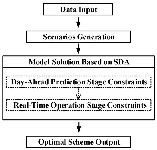
Figure 2.
Flowchart of the steps of the proposed method.
4. Case Study
4.1. System Parameters
In this section, the IEEE 33-node distribution system is used to verify the effectiveness of the proposed method [30], of which the topology is shown in Figure 3. The system contains a total number of 33 nodes and 37 distribution lines, with Node 1 being the substation bus and industrial loads at other nodes. The reference voltage is 12.66 kV and the voltage range is [0.95, 1.05] p.u. The ESS is located at Nodes 11 and 31, each having a capacity of 500 kWh. The maximum charge/discharge power is 100 kW, and the efficiency of charging/discharging is 94%. The PV generation system is located at Nodes 15 and 24, with a capacity of 300 kVA. , , , and are all 0.25. and are set to be 0.4 and 0.6, respectively. , , , , and cost coefficients are set to be 100, 1, 100, 100, 100, and 1, respectively.
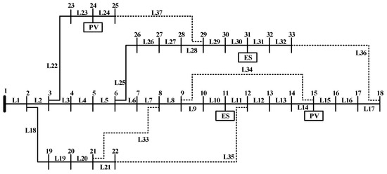
Figure 3.
Topology of the IEEE 33-node distribution system [30].
The PV and load demand prediction curves in the day-ahead prediction stage are shown in Figure 4, respectively. The load demand and solar power output data are based on actual measurements and reliable estimates derived from historical data. The load demand is higher during peak hours (e.g., mornings and evenings) and lower during off-peak hours (e.g., overnight). Conversely, solar power output is typically higher during daylight hours, peaking around midday, and lower or non-existent at night. This alignment with general patterns ensures that the scenarios are representative of real-world conditions.
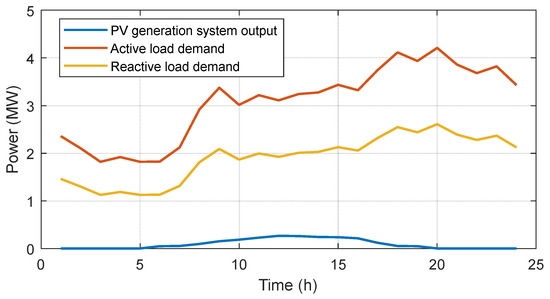
Figure 4.
Prediction curves of the PV and load demand.
A total of four possible PV output and load demand scenarios are considered. The output of PVs and demand of loads for each scenario in the real-time operation stage are, respectively, shown in Figure 5, Figure 6 and Figure 7. The probability of each scenario is 0.4, 0.1, 0.2, and 0.3, respectively. Other parameters are detailed in Ref. [31].
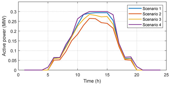
Figure 5.
Possible scenarios of PV output.
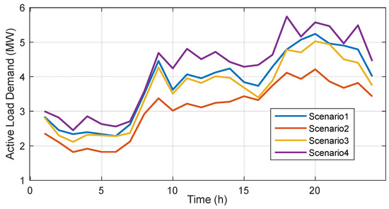
Figure 6.
Possible scenarios of active load demand.
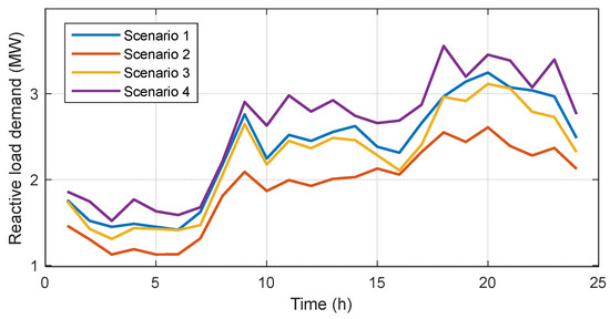
Figure 7.
Possible scenarios of reactive load demand.
The algorithms are compiled in MATLAB (R2014a), modeled using YALMIP (R20230622), and solved using GUROBI (9.5.2). The computer is configured with an Intel Core i5-10400F CPU (Intel, St. Clara, CA, USA) operating at 2.90 GHz and features 16.0 GB of RAM.
4.2. Result Analysis
The result of network reconfiguration is shown in Figure 8. The calculation time is 25,459 s, which is considered acceptable given that the ultimate outcome of this solution is a network reconfiguration plan for the day-ahead prediction stage. It should be noted that the voltage at Node 1, representing the substation node, is not assumed to be a constant but rather dynamically optimized through the coordination and optimization of source-network-load-storage resources.
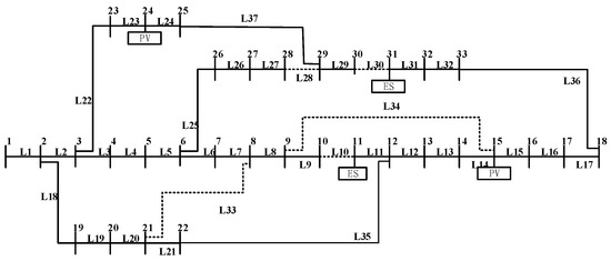
Figure 8.
Network reconfiguration in the day-ahead prediction stage.
In Figure 8, the reconfigured network topology shows the optimized connection between nodes and lines to optimize the voltage across the distribution system.
It is worth mentioning that, the objective function minimizes costs related to wasted PV energy, load loss, ESS operation, and voltage deviation. Constraints ensure stability and safety by regulating network topology, power flows, loads, PV, ESS operations, and so on. During optimization, the objective function adapts to each scenario. For example, in Scenario 4, with high PV output and large load fluctuations, the objective prioritizes minimizing PV energy waste (Equation (41)) by adjusting ESS charging/discharging (Equations (33)–(39)) and PV reactive power (Equations (31) and(32)) to balance supply and demand, while reducing load loss (Equation (43)) and voltage deviation (Equation (44)).
Taking Node 2 as an example (Figure 9), despite fluctuations in PV output and load demand across scenarios, the voltage remains stable within the allowed range (0.95–1.05 p.u.), indicating that the optimization method successfully adjusts PV output, ESS charging/discharging, and network topology to satisfy voltage constraints and minimize costs. Similarly, for Node 17 (Figure 10), the optimization ensures voltage stability across diverse scenarios, demonstrating the effectiveness of the proposed method in balancing costs and ensuring system stability under high PV penetration.
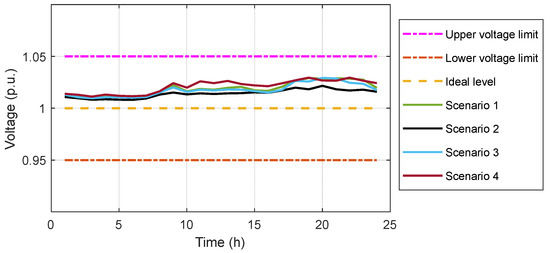
Figure 9.
Voltage of Node 2 in different scenarios.
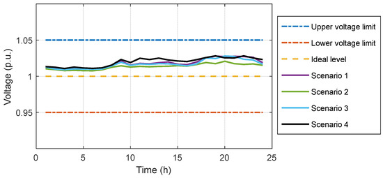
Figure 10.
Voltage of Node 17 in different scenarios.
To elaborate on the results, taking Scenario 4 as an example, the active output of each resource is shown in Figure 11; the total active power of the ESSs and the total actual active PV power are shown in Figure 12; and the total reactive PV power is shown in Figure 13.
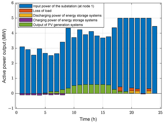
Figure 11.
Output of resources under Scenario 4.
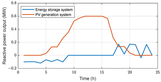
Figure 12.
Active power output of ESSs and PV power generation systems.
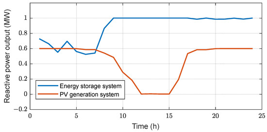
Figure 13.
Reactive power output of ESSs and PV power generation systems.
Combining Figure 6, Figure 11 and Figure 12, it is observable that during the period from 0 h to 8 h, the ESSs are primarily in a charging mode because the active load demand is relatively low. When moving into the 8 h–17 h period, the active load demand starts to increase notably. However, concurrently, the active PV output also experiences a surge. To ensure efficient utilization of PV energy and minimize energy wastage, the ESSs refrain from engaging in significant charging and discharging activities during this timeframe. In the subsequent period, from 17 to 24 h, the active load demand continues to escalate, whereas the PV system’s output starts to decline. To maintain equilibrium between power supply and demand, the ESSs transition into a discharging state. Notably, in Scenario 4, due to the substantial fluctuations in load during this period, the discharging power of the ESSs also exhibits corresponding variations.
Combining Figure 11, Figure 12 and Figure 13, it is observable that, to achieve the effective utilization of PV, the reactive power output is reduced accordingly during the higher active power output period (i.e., time 8 h–17 h) to avoid the waste of PV energy.
Combining Figure 7 and Figure 13, it is obvious that the reactive power output of the ESSs is maintained at a low level during the time period when the load reactive power demand is relatively low (i.e., time 0 h–7 h). However, as the load level increases, the reactive output of the ESS increases accordingly to ensure the voltage quality of the power system.
In order to further verify the effectiveness of the proposed method, the following comparison cases are designed to show its superiority over traditional methods:
- (1)
- Case 1: the proposed model is adopted.
- (2)
- Case 2: the proposed model is adopted without considering network reconfiguration, i.e., the initial topology is fixed.
- (3)
- Case 3: the proposed model is adopted without considering the charging/discharging process of ESSs.
- (4)
- Case 4: the proposed model is adopted without considering the PV output regulation.
The percentages of average voltage deviation across all nodes in the system display notable variations across different scenarios, as shown in Figure 14, Figure 15, Figure 16 and Figure 17. Where, “voltage deviation percent” refers to the percentage deviation of the actual voltage from the nominal or reference voltage at each node in the distribution network. Case 1 exhibits lower voltage deviations in all scenarios, particularly during periods of significant load fluctuations (such as time 17 h–24 h in Scenario 4), where the voltage deviation control effect is particularly notable. In Case 2, the voltage deviation is higher than in Case 1, especially when the network topology is unfavorable for voltage regulation, and the problem of voltage violations is more prominent. In Case 3, although it shows some improvement compared to Case 2, due to the lack of flexible regulation capability of the ESS, the voltage deviation is still relatively large. In Case 4, the absence of photovoltaic output leads to a reduction in system adjustable resources, limited voltage regulation capability, and further increased voltage deviation.
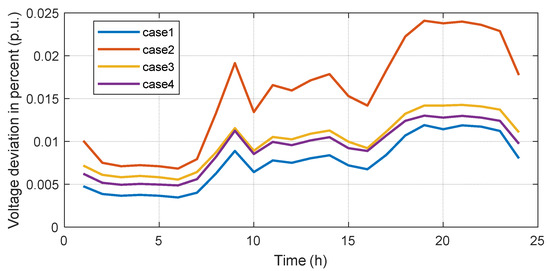
Figure 14.
Percentage of average voltage deviation in Scenario 1 for each case.
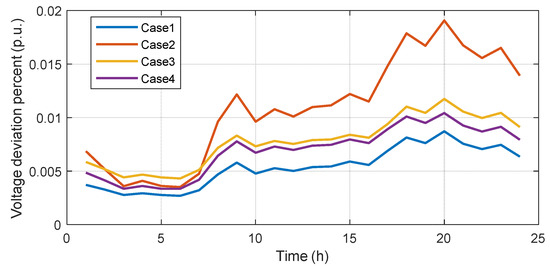
Figure 15.
Percentage of average voltage deviation in Scenario 2 for each case.
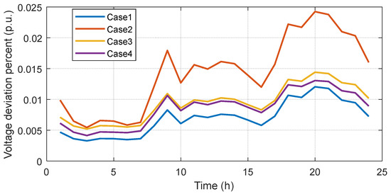
Figure 16.
Percentage of average voltage deviation in Scenario 3 for each case.
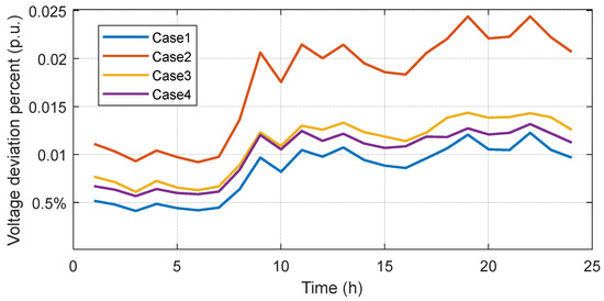
Figure 17.
Percentage of average voltage deviation in Scenario 4 for each case.
The comparative analysis reveals that the crucial elements for achieving voltage optimization in active distribution networks encompass the holistic consideration of coordinated interactions among diverse source-network-load-storage resources, implementing network reconfiguration during the day-ahead phase, and dynamically modulating PV output, ESS operations, and load demand in real-time. The presented approach demonstrates substantial benefits in enhancing voltage quality.
It should be noted that, although the voltage remains within the acceptable limits of 0.95 to 1.05 p.u. in all cases, this is merely the minimum requirement. Even within the acceptable range, deviations from the nominal value can still negatively impact grid stability and equipment operation. Therefore, the optimization ensures that the voltage remains as close as possible to the nominal value (i.e., 1 p.u.), thereby improving voltage quality.
Moreover, the flexibility of the PV system is primarily realized through the reactive power output adjustment of its inverters. The reactive power capability of the inverters enables rapid response to grid voltage fluctuations, optimizing voltage profiles. This adjustment is highly dynamic, responding to real-time grid demands and operational conditions. Due to the inherent uncertainty in the active power output of solar power systems, such as fluctuations caused by weather changes and day-night variations, the integration of ESSs plays a pivotal role. ESSs can absorb excess energy during peak solar generation periods and release it during low-generation times, ensuring a stable power supply and addressing the intermittency of solar power.
5. Conclusions
To tackle the challenge of voltage optimization in active distribution networks characterized by high levels of PV penetration, this study introduces an approach that leverages the synergistic interaction among source, network, load, and storage resources. This approach encompasses distribution network reconfiguration, PV output adjustment, and control of ESSs. The validity is demonstrated using the IEEE 33-node distribution system. The findings reveal that effective coordination and interaction of these resources, both in the day-ahead and real-time stages, can alleviate the impacts of variable renewable energy generation and load fluctuations on distribution network voltage, thereby facilitating the efficient utilization of renewable energy. Comparative analyses further underscore the significance of integrating source, network, load, and storage considerations within the proposed method for both operational phases.
Author Contributions
Conceptualization and methodology, J.L., X.Y. and G.Z.; data curation, W.H. and X.G.; writing—original draft preparation, J.L; writing—review and editing, J.Z. All authors have read and agreed to the published version of the manuscript.
Funding
Innovation Project of China Southern Power Grid Co., Ltd.: Topic 1: Research on coordinated control technology for distribution systems with high penetration of distributed photovoltaic systems (YNKJXM20222334); Topic 4: Practical Verification and Demonstration of Autonomous Control Operation of Distributed Power Supply Areas (YNKJXM20222360).
Data Availability Statement
The data is unavailable due to privacy or ethical restrictions.
Conflicts of Interest
J.L. and X.Y. were employed by Electric Power Institute of Yunnan Power Grid Co., Ltd. J.Z. was employed by Dongchuan Power Supply Bureau of Yunnan Power Grid Co., Ltd. W.H. and X.G. were employed by Kunming Power Supply Bureau of Yunnan Power Grid Co., Ltd. G.Z. was employed by Production and Technology Department of Yunnan Power Grid Co., Ltd. The authors declare that this study received funding from China Southern Power Grid Co., Ltd. The funder was not involved in the study design, collection, analysis, interpretation of data, the writing of this article or the decision to submit it for publication.
Abbreviations
| PV | Photovoltaic |
| DG | Distributed Generator |
| MISOCP | Mixed-integer Second-order Cone Programming |
| SDA | Scenario Decomposition Algorithm |
| ESS | Energy Storage System |
References
- Ma, Y.; Hu, Z.; Song, Y. Hour-ahead optimization strategy for shared energy storage of renewable energy power stations to provide frequency regulation service. IEEE Trans. Sustain. Energy 2022, 13, 2331–2342. [Google Scholar] [CrossRef]
- Guo, X.; Gong, R.; Bao, H.; Wang, Q. Hybrid Stochastic and Interval Power Flow Considering Uncertain Wind Power and Photovoltaic Power. IEEE Access 2019, 7, 85090–85097. [Google Scholar] [CrossRef]
- Vadavathi, A.R.; Hoogsteen, G.; Hurink, J. PV Inverter-based Fair Power Quality Control. IEEE Trans. Smart Grid 2023, 14, 3776–3790. [Google Scholar] [CrossRef]
- Chen, P.; Liu, S.; Wang, X.; Kamwa, I. Physics-shielded Multi-Agent Deep Reinforcement Learning for Safe Active Voltage Control with Photovoltaic/Battery Energy Storage Systems. IEEE Trans. Smart Grid 2022, 14, 2656–2667. [Google Scholar] [CrossRef]
- Sun, X.; Qiu, J.; Yi, Y.; Tao, Y. Cost Effective Coordinated Voltage Control Inactive Distribution Networks with Photovoltaics and Mobile Energy Storage Systems. IEEE Trans. Sustain. Energy 2022, 13, 501–513. [Google Scholar] [CrossRef]
- Reshikeshan, M.; Sree, M.; Matthiesen, L.; Illindala, S.; Renjit, A.; Roychowdhury, R. Autonomous Voltage Regulation by Distributed PV Inverters with Minimal Inter Node Interference. IEEE Trans. Ind. Appl. 2021, 57, 2058–2066. [Google Scholar] [CrossRef]
- Ebrahimi, J.; Eren, S. A Multi-source DC/AC Converter for Integrated Hybrid Energy Storage Systems. IEEE Trans. Energy Convers. 2022, 37, 2298–2309. [Google Scholar] [CrossRef]
- Olivier, F.; Aristidou, P.; Ernst, D.; Cutsem, T. Active Management of Low-Voltage Networks for Mitigating Overvoltages Due to Photovoltaic Units. IEEE Trans. Smart Grid 2016, 7, 926–937. [Google Scholar] [CrossRef]
- Girigoudar, K.; Yao, M.; Mathieu, J.L.; Roald, L.A. Integration of Centralized and Distributed Methods to Mitigate Voltage Unbalance Using Solar Inverters. IEEE Trans. Smart Grid 2022, 14, 2034–2046. [Google Scholar] [CrossRef]
- Chen, M.; Gong, X.; Liang, Z.; Zhao, J.; Tian, Z. Bi-Hierarchy Capacity Programming of Co-Phase TPSS with PV and HESS for Minimum Life Cycle Cost. Int. J. Electr. Power Energy Syst. 2023, 147, 108904. [Google Scholar] [CrossRef]
- Zhang, B.; Tang, W.; Cai, Y.; Wang, Z.; Li, T.; Zhang, H. Consensus Algorithm Distributed Control Strategy of Residential Photovoltaic Inverter and Energy Storage Based on Consensus Algorithm. Autom. Electr. Power Syst. 2020, 44, 86–94. [Google Scholar] [CrossRef]
- Jothibasu, S.; Dubey, A.; Santoso, S. Two-stage Distribution Circuit Design Framework for High Levels of Photovoltaic Generation. IEEE Trans. Power Syst. 2018, 34, 5217–5226. [Google Scholar] [CrossRef]
- Mahdavi, M.; Schmitt, K.; Chamana, M.; Jurado, F.; Bayne, S.; Marfo, E.A.; Awaafo, A. A Mixed-Integer Programming Model for Reconfiguration of Active Distribution Systems Considering Voltage Dependency and Type of Loads and Renewable Sources. IEEE Trans. Ind. Appl. 2024, 60, 5291–5303. [Google Scholar] [CrossRef]
- Yue, D.; He, Z.; Dou, C. Cloud-Edge Collaboration-Based Distribution Network Reconfiguration for Voltage Preventive Control. IEEE Trans. Ind. Inform. 2023, 19, 11542–11552. [Google Scholar] [CrossRef]
- Hu, X.; Liu, Z.; Wen, G.; Yu, X.; Liu, C. Voltage Control for Distribution Networks via Coordinated Regulation of Active and Reactive Power of DGs. IEEE Trans. Smart Grid 2020, 11, 4017–4031. [Google Scholar] [CrossRef]
- Ranamuka, D.; Agalgaonkar, A.P.; Muttaqi, K.M. Online Coordinated Voltage Control in Distribution Systems Subjected to Structural Changes and DG Availability. IEEE Trans. Smart Grid 2015, 7, 580–591. [Google Scholar] [CrossRef]
- Yang, M.; Liu, Y.; Guo, L.; Wang, Z.; Zhu, J.; Zhang, Y. Hierarchical Distributed Chance-constrained Voltage Control for HV and MV DNs Based on Nonlinearity-Adaptive Data-driven Method. IEEE Trans. Power Syst. 2024, 1–14. [Google Scholar] [CrossRef]
- Zhan, Q.; Su, J.; Lin, J.; Guo, S. Coordinated Optimization of Source–Storage–Load in Distribution Network Based on Edge Computation. Energy Rep. 2023, 9, 492–498. [Google Scholar] [CrossRef]
- Park, J.Y.; Ban, J.; Kim, Y.J.; Catalao, J.P. Supplementary Feedforward Voltage Control in a Reconfigurable Distribution Network Using Robust Optimization. IEEE Trans. Power Syst. 2022, 37, 4385–4399. [Google Scholar] [CrossRef]
- Gao, X.; Zhang, J.; Sun, H.; Liang, Y.; Wei, L.; Yan, C.; Xie, Y. A Review of Voltage Control Studies on Low Voltage Distribution Networks Containing High Penetration Distributed Photovoltaics. Energies 2024, 17, 3058. [Google Scholar] [CrossRef]
- Vijayan, V.; Mohapatra, A.; Singh, S.N.; Dewangan, C.L. An Efficient Modular Optimization Scheme for Unbalanced Active Distribution Networks with Uncertain EV and PV Penetrations. IEEE Trans. Smart Grid 2023, 14, 3876–3888. [Google Scholar] [CrossRef]
- Shen, Y.; Qian, T.; Li, W.; Zhao, W.; Tang, W.; Chen, X.; Yu, Z. Mobile Energy Storage Systems with Spatial–temporal Flexibility for Post-disaster Recovery of Power Distribution Systems: A Bilevel Optimization Approach. Energy 2023, 282, 128300. [Google Scholar] [CrossRef]
- Zhang, Z.; Zhang, Y.; Yue, D.; Dou, C.; Ding, L.; Tan, D. Voltage Regulation with High Penetration of Low-Carbon Energy in Distribution Networks: A Source–Grid–Load-Collaboration-Based Perspective. IEEE Trans. Ind. Inform. 2021, 18, 3987–3999. [Google Scholar] [CrossRef]
- Cararo, J.A.G.; Caetano, N.J.; Vilela, W.A., Jr. Spatial Model of Optimization Applied in the Distributed Generation Photovoltaic to Adjust Voltage Levels. Energies 2021, 14, 7506. [Google Scholar] [CrossRef]
- Ding, T.; Sun, K.; Huang, C.; Bie, Z.; Li, F. Mixed-integer Linear Programming-based Splitting Strategies for Power System Islanding Operation Considering Network Connectivity. IEEE Syst. J. 2018, 12, 350–359. [Google Scholar] [CrossRef]
- Ding, T.; Lin, Y.; Li, G.; Bie, Z. A New Model for Resilient Distribution Systems by Microgrids Formation. IEEE Trans. Power Syst. 2017, 32, 4145–4147. [Google Scholar] [CrossRef]
- Alshammari, M.; Duffy, M. Review of Single-Phase Bidirectional Inverter Topologies for Renewable Energy Systems with DC Distribution. Energies 2022, 15, 6836. [Google Scholar] [CrossRef]
- Feng, T.; Wang, C.; Chen, S. Optimal Scheduling of Active Distribution Network Considering Energy Storage System and Reactive Compensation Devices. In Proceedings of the 2021 IEEE Industry Applications Society Annual Meeting (IAS), Vancouver, BC, Canada, 10–14 October 2021; pp. 1–10. Available online: https://ieeexplore.ieee.org/document/9677052 (accessed on 17 January 2022).
- Ahmed, S. A Scenario Decomposition Algorithm for 0-1 Stochastic Programs. Oper. Res. Lett. 2013, 41, 565–569. [Google Scholar] [CrossRef]
- Lin, Y.; Bie, Z. Tri-level Optimal Hardening Plan for a Resilient Distribution System Considering Reconfiguration and DG Islanding. Appl. Energy 2018, 210, 1266–1279. [Google Scholar] [CrossRef]
- Baran, M.E.; Wu, F.F. Network Reconfiguration in Distribution Systems for Loss Reduction and Load Balancing. IEEE Trans. Power Deliv. 1989, 4, 1401–1407. [Google Scholar] [CrossRef]
Disclaimer/Publisher’s Note: The statements, opinions and data contained in all publications are solely those of the individual author(s) and contributor(s) and not of MDPI and/or the editor(s). MDPI and/or the editor(s) disclaim responsibility for any injury to people or property resulting from any ideas, methods, instructions or products referred to in the content. |
© 2024 by the authors. Licensee MDPI, Basel, Switzerland. This article is an open access article distributed under the terms and conditions of the Creative Commons Attribution (CC BY) license (https://creativecommons.org/licenses/by/4.0/).