Abstract
Aiming at the problem of accurate AC series arc fault detection, this paper proposes a low voltage AC series arc fault intelligent detection model based on deep learning. According to the GB/T 31143—2014 standard, an experimental platform was established. This system comprises a lower computer (slave computer) and an upper computer (master computer). It facilitates the acquisition of experimental data and the detection of arc faults during the data acquisition process. Based on a one-dimensional Convolutional Neural Network (CNN), Residual model (Res) and RIME optimization algorithm (RIME) are introduced to optimize the CNN. The current signals collected using high-frequency current, low-frequency coupled current, and high-frequency coupled current are used to construct an arc fault feature set for training of the necessary detection model. The experimental results indicate that the RIME optimization algorithm delivers the best performance when optimizing a one-dimensional CNN detection model with an introduced Res. This model achieves a detection accuracy of 99.42% ± 0.13% and a kappa coefficient of 95.69% ± 0.96%. For collection methods, high-frequency coupled current signals are identified as the optimal choice for detecting low-voltage AC series arc faults. Regarding feature selection, random forest-based feature importance ranking proves to be the most effective method.
1. Introduction
Due to the impact of different circuit and load types, the current magnitude associated with arc faults varies. Series arc faults, in particular, generate lower currents compared to parallel and ground arc faults, making them more difficult for circuit breakers to detect. This challenge in detection can prevent timely circuit disconnection, increasing the risk of electrical fires. Therefore, effective intelligent detection of AC series arc faults under various operating conditions is critical for reducing the likelihood of electrical fires. Currently, arc fault detection methods are categorized into three main types:
1.1. Fault Arc Detection Method Based on Mathematical Modeling
Traditional arc models are used to describe the electrical characteristics, behavior, and impact of arcs for fault detection and protection in power systems. Common models include the empirical model, Elmore model, Sato model, and Mayr model. Each model has its own strengths and limitations, and the choice of model depends on the specific application requirements, operating conditions, and desired accuracy. In practice, it may be beneficial to combine multiple models or techniques to improve the accuracy and reliability of arc fault detection. D. Lee and J. Kim conducted empirical modeling of arc faults based on the latest experimental data and field studies [1], T. Carter and J. Wang analyzed the influence of a high-current arc fault on a power system based on the Elmore model [2], K. Nakamura and H. Nakajima discussed the improvement of arc fault detection based on the Sato model and combined with machine learning methods for optimization [3], and G. Yang, T. Li and X. Zhang reviewed the progress of arc fault detection methods and discussed the application of the Mayr model in arc fault detection [4]. Although the traditional arc model can simulate the characteristics of an arc, it still cannot reflect the intermittency of an arc.
The arc fault detection method based on mathematical modeling needs to use a large number of parameters to describe and define arc characteristics. With the continuous research on arc faults, the types of arc fault models are increasing, and the number of model parameters used is also increasing. However, all model parameters cannot be accurately obtained through test data. The purpose of this method is just to study the mechanism of arc generation and provide a theoretical basis for arc detection.
1.2. Fault Arc Detection Method Based on Physical Signals
Physical signals include arc light [5], arc sound [6], electromagnetic radiation [7,8], and changes in ambient temperature and pressure caused by an arc [9,10]. When the above characteristics of the arc are detected, the arc fault can be determined. C.D. Johnson discussed the practical application of using optical sensors to detect arc faults. The research focuses on the design, performance evaluation, and effectiveness of optical sensors in power systems [11], M.R. Brown and H.A. Lee introduced the application of acoustic emission technology in arc fault detection, including the feature analysis of acoustic emission signals and the improvement of fault diagnosis methods [12], and D.A. Johnson discussed the application of electromagnetic sensors in power systems, especially how to use electromagnetic radiation signals for arc fault detection. The research includes the design, performance analysis, and application cases of electromagnetic sensors [13]. E.K. Smith and L.Y. Zhao introduced the method of arc fault detection using ambient temperature and pressure sensors. The research includes the performance evaluation of the sensor and its effect in practical applications [14].
Usually the wire is closed in the wall, not exposed on the surface of the wall, and the associated physical signal generated by the arc is absorbed by the wall. Difficult to observe, this method is only suitable for electric meter boxes, electrical cabinets, and other specific occasions which are difficult to promote in the household electricity environment. At the same time, this method has some problems such as low sensitivity, detection delay, complex structure, and easy interference by other signal sources.
1.3. Fault Arc Detection Method Based on Electrical Signals
With the increasing variety of household appliances, arcs can occur during their operation, and the distribution of these appliances is random. This randomness makes it challenging to pinpoint the exact location of an arc fault. When an arc fault occurs, the current and voltage signals in the circuit become distorted and are not necessarily indicative of the arc’s location. Therefore, detecting arc faults by measuring the circuit’s current and voltage signals has become a widely used method. Current research focuses on signal selection, effective feature extraction, and intelligent recognition using machine learning models.
The voltage signal, low frequency current signal, high frequency current signal, and coupling current signal can be selected for a low voltage AC series arc fault. S.J. Park and K.H. Kim discussed the analytical method and experimental results for the arc fault detection of voltage signals in low voltage AC systems [15], L.M. Zhang and Y.X. Wang studied the characteristics of low frequency current signals in series arc faults of low voltage AC circuits and proposed corresponding detection methods [16], H.R. Lee and J.P. Choi discussed the application of high frequency current signals in detecting series arc faults in low voltage AC networks [17], and M.T. Liu and F.L. Zhang studied the method and effect of coupling current signals in identifying series arc faults in low voltage AC systems [18].
The extraction of effective features involves deriving time-domain, frequency-domain, and time-frequency domain characteristics from the collected signals. Techniques such as Fourier transform [19], wavelet packet transform [20], empirical mode decomposition [21], variational mode decomposition [22], and complete ensemble empirical mode decomposition [23] are employed to extract different modal features from the signals. These features are then used as inputs for the arc fault detection model. L.M. Zhao and R.T. Hu reviewed the application of multi-modal feature extraction and intelligent detection techniques in arc fault detection. It highlights advanced signal processing techniques such as Fourier transform, wavelet packet transform, empirical mode decomposition, variational mode decomposition, and complete ensemble empirical mode decomposition. The article discusses how these techniques are used to extract time-domain, frequency-domain, and time-frequency domain features from arc fault signals. The paper highlights the potential of integrating advanced signal processing techniques with intelligent detection models. These combined methods can significantly improve the accuracy and reliability of arc fault detection, which is crucial for practical applications [24].
The extracted time-domain, frequency-domain, and time-frequency domain features serve as inputs for the arc fault detection model. Feature dimensionality reduction is performed using Principal Component Analysis (PCA) [25], and Kernel Principal Component Analysis (KPCA) [26]. Feature selection, using random forest importance ranking, reduces data redundancy and decreases the computational load of the detection model. Fault identification can be achieved by setting empirical thresholds or by using neural network models such as a Backpropagation Neural Network (BPNN) [27], Extreme Learning Machine (ELM) [28], Probabilistic Neural Network (PNN) [29], and Fully Connected Neural Network (FCNN) [30]. Machine learning models such as a Support Vector Machine (SVM), decision tree, and random forest, along with deep learning models such as a CNN, deep neural network, and recurrent neural network, can also be employed as arc fault detection models to achieve high detection accuracy. Incorporating residual connections, attention mechanisms, and depth wise separable convolutions in deep learning-based detection models can prevent vanishing and exploding gradient issues in deep networks. This approach reduces computational complexity and decreases network model parameters and prediction time while enhancing detection accuracy, generalization, and robustness. Optimization algorithms such as the Genetic Algorithm (GA), Particle Swarm Optimization (PSO), the Sparrow Search Algorithm (SSA), and the Firefly Algorithm (FA) can further improve detection accuracy. Lu Xing proposed a deep learning method for diagnosing series DC arc faults and predicting circuit behavior. It uses time-frequency slices from power supply signals to extract features. A CNN captures static features, while a long short-term memory network (LSTM) captures dynamic features. The method was tested on simulated DC arcs, achieving 98.43% accuracy and accurate time-domain predictions [31].
Different electrical signals have a significant impact on the effectiveness of series arc fault detection. Each signal type provides unique arc information that influences the validity of the extracted features. The complexity and specificity of feature extraction affect the difficulty of the detection model. While highly specific features enhance the accuracy and sensitivity, they can also increase the computational demands if they are too complex. Therefore, features need to balance specificity and simplicity, and the detection model must achieve high accuracy. The model should perform well in the current experimental environment, with data that not only meets national standards but also simulates typical household conditions. Thus, optimizing signal acquisition methods, quantifying arc characteristics, and developing precise detection models are the key challenges in low-voltage AC series arc fault detection. Effectively addressing these challenges is a major focus of current research.
According to the above large amount of literature, we can summarize the advantages and disadvantages of three kinds of arc detection methods, as shown in Table 1.

Table 1.
Comparison of arc detection methods.
Table 1 above is a comparison of the advantages and disadvantages of the three arc fault detection methods. Through the comparison of various advantages and disadvantages, the use of electrical signals for arc signal detection is easy to observe, less sensors are required, and the cost is low. Combined with the actual needs of the low-voltage AC series arc fault detection, this paper will use electrical signals for arc signal detection.
2. Arc Fault Detection Model
There are many types of arc fault detection models. This paper proposes a low-voltage AC series arc detection model based on a one-dimensional convolutional neural network incorporating residual modules and the frost optimization algorithm. This detection model uses extracted time-domain, frequency-domain, and wavelet packet energy features as inputs. It was trained, validated, and tested on an established experimental data set. Experimental results show that this arc fault detection model has high detection accuracy.
2.1. Series Arc Fault Detection Model Based on Convolutional Neural Network
A CNN is a type of feedforward neural network. It has the characteristics of sparse connectivity, shared weights, and spatial secondary sampling, which simplifies the input dimension, improves the speed of network training, and simplifies the algorithm flow. Since its inception, the CNN has extended a variety of network models, which have been successfully applied in various fields, and many research results and conclusions have appeared in various fields. The optimization of the CNN by scholars focuses on the structural improvement of the CNN network model and the optimization of training methods. Optimization of the network structure is achieved by adding some structures to the construction of the CNN network to increase the feature extraction ability or classification and prediction ability of the CNN. The optimization of the network training algorithm includes the selection and adjustment of hyperparameters.
A CNN consists of multiple network layers in series, and the network structure generally includes an input layer, hidden layer, and output layer. The input layer receives the raw information of the input data. The hidden layer transforms the data linearly based on the relationship between the input data and the output data, including the convolution layer, pooling layer, batch normalization layer, and nonlinear excitation layer. The output layer includes the classification results of the output model, including the fully connected layer, SoftMax layer for classification, and classification layer. The CNN network structure is shown in Figure 1.
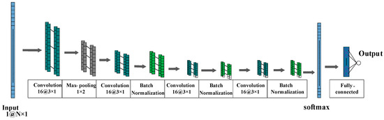
Figure 1.
CNN structure.
The convolution layer uses convolution cores to scan the input layer to extract features. Each convolution layer can set multiple convolution cores. The specific parameters of these convolution cores can be adaptively learned through the training process, and different convolution cores can be set to extract different features. The pooling layer reduces the feature dimension extracted by the convolutional layer through the down sampling operation. Two methods can be selected: the maximum pooling method selects the maximum output of the data within the sampling range, and the mean pooling method selects the arithmetic average output of all non-zero data within the sampling range. Both pooling methods not only reduce the network dimension, but also reduce the network dimension. Moreover, the invariance of several features is maintained to prevent overfitting of the network. The nonlinear excitation layer uses activation functions to extract features from the output data of the convolution layer and the pooling layer. The commonly used activation functions are the Sigmoid function, Tanh function, and Relu function. The Relu function does not cause the network gradient to disappear compared to the Sigmoid function and the Tanh function. The full connection layer connects the classification layer, which outputs the network classification results.
2.2. Convolutional Neural Network Series Arc Fault Detection Model Based on Residual Module
Neurons connect the front and back layers of the neural network. Each layer of the neural network receives the linear mapping of the previous layer and uses the activation function to nonlinearly activate the output of this layer, and the activation function connects the weights between neurons, giving the neural network the ability to nonlinearly fit various complex data. In the process of network training, the backpropagation algorithm based on the gradient descent strategy is adopted generally. In addition, the parameters to be trained are updated based on the negative gradient direction of the objective function. When a deep CNN is designed, the number of new parameters will increase rapidly when the number of network layers increases, and problems such as network degradation, gradient explosion, and gradient disappearance occur easily during network training. Res can overcome this problem.
The Res can not only deepen the network structure by increasing the number of network layers, but also improve the network degradation and gradient disappearance caused by too deep a network structure. In addition, it can also improve the generalization ability of the network model. In this paper, the Res is introduced to optimize the low voltage AC series arc fault detection model based on a one-dimensional CNN without increasing the number of network parameters and calculations.
The structure of the Res is shown in Figure 2, whereby x represents the input signal of the upper layer of the neural network, y represents the output signal of the next layer of the neural network, F(x) represents the mapping function in the Res, and the activation function adopts Relu. The actual mapping mode in the Res can be expressed as , which means that the problem of fitting y directly becomes fitting the residual function F(x). When F(x) is 0, the best mapping solution y is obtained. This mapping method makes it easier to train the fault arc detection model in this chapter and also avoids the problems of training degradation and gradient disappearance. Figure 3 shows the network structure of a Res-1DCNN.
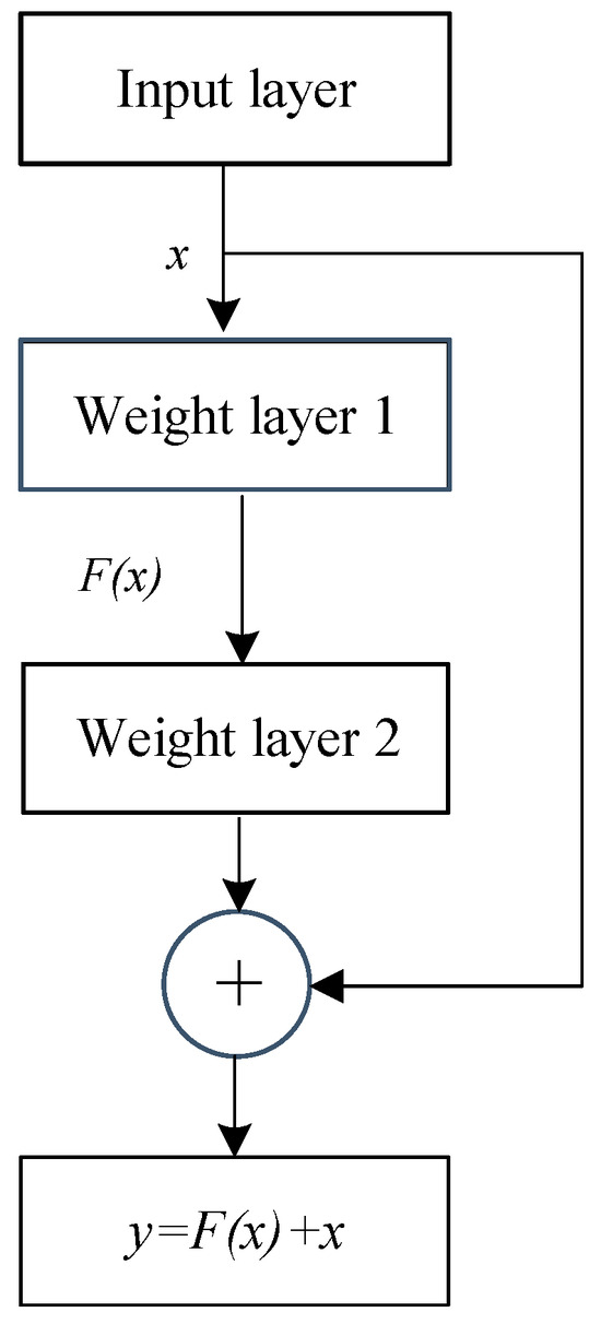
Figure 2.
Res structure diagram.
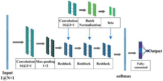
Figure 3.
Res-1DCNN network structure diagram.
2.3. Convolutional Neural Network Series Arc Fault Detection Model Based on the RIME Optimization Algorithm
Optimization algorithms are methods, either stochastic or deterministic, designed to minimize or maximize single, multiple, or multi-objective functions by taking into account gradient information, constraints, or the priorities of the system or decision-maker. The RIME optimization algorithm, introduced by Su Hang in February 2023, is an efficient optimization algorithm inspired by the physical phenomenon of RIME formation. By simulating the motion of soft RIME particles, the RIME algorithm employs a unique stepwise exploration and exploitation strategy, allowing it to continuously switch between large-scale exploration and small-scale exploitation. This ensures both breadth and depth in the search for the optimal solution, achieving high efficiency and precision. The algorithm also introduces the hard RIME particle puncture mechanism, inspired by the crossing behavior between hard RIME particles. This mechanism allows the RIME algorithm to quickly lock onto a globally approximate optimal solution. By dimensionally crossing and exchanging information between the optimal solution and the current solution, the precision and efficiency of the solution are significantly improved. Furthermore, the forward greedy selection mechanism enables the RIME algorithm to actively adjust the position of the frost agent, filtering out inferior solutions within the population. By altering the selection of the optimal solution, suboptimal solutions are proactively introduced, enhancing the diversity of the population while maintaining its quality. This reduces the risk of the algorithm becoming trapped in local optima. The RIME algorithm’s innovative approach leverages the natural behaviors of RIME formation to provide a balanced and dynamic optimization process, ensuring robust performance across various optimization scenarios.
Compared to other optimization algorithms, the RIME has the following unique characteristics:
- Dynamic adaptability: simulates the freezing and thawing processes of frost and ice, allowing it to flexibly adapt to changing environments and avoid local optima.
- Diversity maintenance: maintains population diversity through the state changes of frost and ice, enhancing global search capability.
- Efficient local search: the thawing process improves the fine-grained local search ability, leading to a higher solution quality.
- Simplicity and ease of implementation: features a simple structure with fewer parameters, making it easy to implement and tune.
- Fast convergence: an efficient search mechanism that enhances the algorithm’s convergence speed and optimization performance.
These characteristics make RIME highly advantageous in solving complex optimization problems.
The RIME population is initialized, and the position of RIME particles is calculated according to Equation (1).
where is the new position of the updated RIME particle, is the frost agent, and is the RIME particle. is the best frosting agent in RIME population R. The parameter r1 is a random number in the range of (−1, 1). r1 controls the movement direction of RIME particles. changes with the increase of iterations. β is an environment factor, which simulates the influence of the external environment through the change of iteration times to ensure the convergence of the algorithm. h is a random number in the range of (0, 1), which is used to control the distance between the center of two frost and ice particles. and are the upper and lower bounds of the escape space, respectively, which limit the effective regions of RIME particles. E is the adhesion coefficient of RIME particles, which affects the condensation probability of the frost agent and increases with the increase of iterations. r2 is a random number in the circle, which together with E controls whether the RIME particles condense, that is, whether the particle position is updated.
θ is calculated via Equation (2):
where t is the current iteration number and T is the maximum iteration number of the algorithm.
Through Equation (3), we can calculate β:
where β is the step function, [•] indicates rounding, and w defaults to 5 to control the number of segments of the step function.
E is calculated via Equation (4):
where t is the current iteration number and T is the maximum iteration number of the algorithm.
A flow chart of the RIME optimization algorithm is shown in Figure 4.
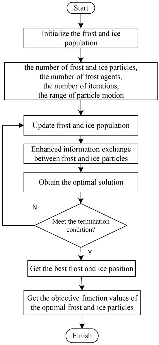
Figure 4.
Flow chart of RIME optimization algorithm.
3. Performance Evaluation Index of Series Arc Fault Detection Model
The detection accuracy of a well-built and trained low-voltage AC series arc fault detection model is related to the algorithm, data, and tasks in the model, so it is very important to evaluate the performance of the detection model. The selection of accurate evaluation indicators and the use of different evaluation systems have a great impact on the evaluation results. In this paper, some indexes are selected as standards to evaluate the performance of the arc detection model and verify the effectiveness of the classification accuracy of the designed arc detection model. In this paper, specificity (Sp), sensitivity (Se), accuracy (Ac), and kappa coefficient (KC) were selected as evaluation indexes for classification performance of the classifier.
Sp represents the accuracy rate of recognition for each category, which is the proportion of the number of arc states classified as arc states in the sum of the number of arc states classified as normal and the number of arc states classified as arc states, also known as the true negative rate. The higher the specificity, the higher the accuracy rate. The specificity is calculated as shown in Equation (5):
Se represents the recognition ability of the designed classification model. It is the proportion of the number of recognition results classified as being in a normal working state to the sum of the number of recognition results classified as being in a normal working state and the number of recognition results classified as being in a normal arc state, also known as the true positive rate. The higher the sensitivity, the higher the accuracy of recognition. Sensitivity represents the recognition ability of the designed model, and the calculation formula is shown in Equation (6):
Ac represents the correct results predicted by the classification model. It is the proportion of the sum of the number of recognition results classified as being in a normal working state and the number of recognition results classified as being in an arc state to the total number of samples. The higher the accuracy, the higher the correct rate of recognition. The accuracy calculation formula is shown in Equation (7):
Among them, TP, FP, FN, and TN are the true positive, false positive, false negative, and true negative of the classification results. TP is the number of recognition results whereby the normal working state is classified into the normal state; FP is the number of recognition results whereby the arc state is classified into the normal state; FN is the number of recognition results whereby the normal state is classified into the arc state; TN is the number of recognition results whereby the arc state is classified into the arc state.
KC is used to test consistency and measure the classification effect, that is, whether the predicted classification result of the model is consistent with the actual classification result. Its calculation formula is shown in Equations (8)–(10):
where is the ratio of the sum of the diagonal elements of the confusion matrix to the sum of the whole elements of the confusion matrix, that is, the accuracy; is the ratio of the sum of the product of the actual and predicted quantities corresponding to all categories respectively to the square of the total number of samples; r is the number of rows of the confusion matrix; is the sum of all elements on row t; is the sum of all elements on column t.
is the kappa coefficient corresponding to each classification result, and its calculation formula is shown as Equations (11)–(14):
The higher the values of the four performance measures—Sp, Se, Ac, and KC—the better the overall recognition performance of the classifier. A higher Sp means a higher probability of correctly identifying the negative class. A higher Se indicates a lower probability of missed detection (false negative). The KC has a value between (0, 1), where a value closer to 1 indicates that the classifier is more accurate compared to random classification. Ac reflects the overall correct classification rate of the classifier across all samples. However, these metrics do not have the same evaluation weighting factor. In different application scenarios, some metrics may be more important than others. For example, in medical diagnosis, reducing missed diagnoses (i.e., higher sensitivity) is often more critical While in financial fraud detection, reducing the false positive rate, that is, higher specificity, may be of greater concern. Therefore, the weighting factors of performance indicators will be adjusted according to different problem backgrounds and requirements. In this subject, these four performance indicators are essential, so these four indicators will be integrated into the analysis of the experimental results. If the four indicators are high, it means that the corresponding algorithm has better performance.
4. Experimental Results and Analysis
Figure 5 shows the physical setup of the slave computer for the arc fault detection system. When the power is activated, the red power indicator light turns on. Adjusting the horizontal adjustment knob on the arc generator brings the fixed and moving electrodes into close proximity. This will cause the green status indicator light to illuminate. Once the load is connected and the appliance switch is turned on, signals from the appliance in its normal operating state can be collected. By rotating the adjustment knob to gradually separate the fixed and moving electrodes, an arc will be generated, allowing for the collection of signals from the appliance in an arcing state.
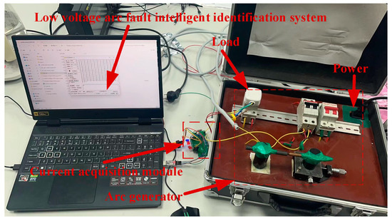
Figure 5.
Physical setup of the lower computer for the arc fault detection system.
The master computer of the low-voltage AC series arc fault detection system consists of a signal reception module and a signal storage module. Its main function is to receive current signals collected by the slave computer and store the received signals. The system uses a PC equipped with LabVIEW software to develop the interface, connecting with the Bluetooth communication module in the experimental data acquisition platform to achieve data reception, transmission, and storage. Figure 6 shows the interface of the low-voltage AC series arc fault acquisition system, based on LabVIEW software, designed in this paper.
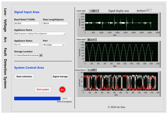
Figure 6.
Low-Voltage AC Series Arc Fault Acquisition System Interface.
Based on 1DCNN, a residual connection is introduced in this project, and a RIME optimization algorithm is used to optimize the initial learning rate and the optimal number of nodes of the hidden layer of the detection model. The structure of the CNN model is shown in Figure 3, and the specific parameters of the network structure are shown in Table 2. These include the number of layers in the network, the size, number, step size of the convolution kernel, and the activation function used.
Table 2.
Optimized detection model network structure.
Among them, the pixel size of the input layer is determined by the dimension of the established arc fault feature set. When the feature set without feature reduction and selection is used as the input, N is set to 22, and different values of N are obtained after feature reduction and feature selection via different methods for different current signals collected.
The Adam optimization algorithm was used to train the designed low-voltage AC series arc fault detection model. Four performance evaluation indexes of the detection model, namely, specificity, sensitivity, accuracy, and kappa coefficient, were used to measure the performance of the fault arc detection model. Different optimization algorithms would have certain influence on the detection accuracy under different models. Adaptive Moment Estimation (Adam) is used to dynamically adjust the learning rate of each parameter of the CNN model. This algorithm can dynamically adjust the learning rate according to the change of gradient. The Adam algorithm has the fastest convergence speed and the smallest loss rate, indicating that it is easier to converge when training large-scale data sets and complex networks, and its convergence speed is also the fastest.
In this study, four kinds of low-voltage AC series arc fault detection models based on CNN were designed and compared, and the optimal low-voltage AC series arc fault detection model was selected. The design models include: 1DCNN, Res-1DCNN, a one-dimensional convolutional neural network optimized via a RIME optimization algorithm (RIME-1DCNN), and a one-dimensional convolutional neural network optimized via a RIME optimization algorithm with a residual model (RIME-Res-1DCNN) introduced. The parameter settings of four fault arc detection algorithm models based on CNNs are shown in Table 3.
Table 3.
Detect algorithm model parameters.
With the established arc fault feature set as input, four kinds of low-voltage AC series arc fault detection models based on CNNs were trained, verified, and tested. According to the experimental results obtained, the experimental results of the four detection models were analyzed and compared, and each evaluation index of the four algorithm models was obtained, and the influence of Res and the RIME optimization algorithm on the performance of the detection model was further analyzed.
The high frequency current feature set, low frequency coupled feature set, and high frequency coupled feature set without feature reduction and feature selection were used as the input of the four models designed, and the training, verification, and testing were carried out, respectively. The model detection accuracy was evaluated using the performance evaluation index of the series arc fault detection model. The optimal arc fault feature set was selected by comparing and analyzing the experimental data obtained.
Three feature sets, namely, Principal Components Analysis (PCA) for feature reduction, Mean Impact Value (MIV) for feature selection and Random Forest (RF) for feature selection, were used as inputs to the four models designed and were trained, verified, and tested, respectively. The model detection accuracy was evaluated using the performance evaluation index of the series arc fault detection model. Compared with the experimental results of three feature sets without feature reduction and feature selection, the optimal feature reduction and feature selection method was obtained.
All established arc fault feature sets were divided into two categories: the label of the normal working state was set to 1, and the label of the pulled arc state was set to 2. In the training process of the CNN algorithm model, it is very important to select an optimizer suitable for the algorithm model to guide the learning of the parameters. In this chapter, the Adam optimization algorithm is used to train the four low-voltage AC series arc fault detection models. Four performance evaluation indexes of the detection model, namely, specificity, sensitivity, accuracy, and kappa coefficient, were used to measure the performance of the fault arc detection model. Different optimization algorithms would have certain influence on the detection accuracy under different models. The four fault arc detection algorithm models obtained on the training set and the verification set were tested on the test set, respectively, and the performance evaluation index of each algorithm model was obtained. The performance indicators obtained via the four fault arc detection algorithm models were compared, and the experimental comparison results are shown as follows.
The arc fault feature set was established by extracting features from 4308 sets of high-frequency current signals with the length of one-fifth of the sampling frequency as a window. For the high-frequency current signals without feature reduction and feature selection, the size of the feature set was 22 × 24,713. The constructed feature set was used as the input of the four detection models. Ten thousand samples in the feature set were used as the training set for model training, and the remaining samples were used as the test set. The experimental results obtained using the four performance evaluation indicators of the detection model are shown in Table 4.
Table 4.
Experimental results of high frequency current feature set.
According to the experimental results obtained in Table 3, the RMIE-Res-1DCNN model can obtain the best detection performance for the collected high-frequency current signals. This model has the highest specificity, sensitivity, accuracy, and kappa coefficient. By comparing the 1DCNN model and Res-1DCNN model, it can be seen that the sensitivity, specificity, accuracy, and Kappa coefficient of the model are significantly improved after the introduction of the Residual Network (ResNet). By comparing the 1DCNN model and RMIE-1DCNN model, it can be seen that the detection performance of the CNN model is improved by using the RIME optimization algorithm, the feature set is more stable on the model, and the variation range of the obtained performance indicators is smaller.
The arc fault feature set was established by extracting features from 4308 sets of high-frequency current signals with a length of one-fifth of the sampling frequency as a window. For the high-frequency current signals with feature dimensionality reduction via PCA, the size of the feature set was 12 × 24,713. The constructed feature set was used as the input of the four detection models. Ten thousand samples in the feature set were used as the training set for model training, and the remaining samples were used as the test set. The experimental results obtained using the four performance evaluation indicators of the detection model are shown in Table 5.
Table 5.
Experimental results of high frequency current feature set—PCA.
According to the experimental results obtained in Table 4, the RMIE-Res-1DCNN model can obtain the best detection performance for the collected high-frequency current signals. Although the feature dimensionality reduction using PCA will cause the loss of original information, it does not reduce the detection accuracy of the model and reduces the redundancy of data and improves the training speed of the model.
The arc fault feature set was established by extracting features from 4308 sets of high-frequency current signals with the length of one-fifth of the sampling frequency as a window. For the high-frequency current signals with MIV for feature selection, the size of the feature set was 8 × 24,713. The constructed feature set was used as the input of the four detection models. Ten thousand samples in the feature set were used as the training set for model training, and the remaining samples were used as the test set. The experimental results obtained using the four performance evaluation indicators of the detection model are shown in Table 6.
Table 6.
Experimental results of high frequency current feature set—MIV.
According to the experimental results obtained in Table 5, the RMIE-Res-1DCNN model can obtain the best detection performance for the collected high-frequency current signals. Using MIV for feature selection, features with higher importance and richer original information were selected, resulting in less loss of original information, not reducing the detection accuracy of too many models, and reducing the redundancy of data to improve the training speed of the model.
The arc fault feature set was established by extracting features from 4308 sets of high-frequency current signals with a length of one-fifth of the sampling frequency as a window. The size of the feature set was 8 × 24,713 for high-frequency current signals with RF feature selection. The constructed feature set was used as the input of the four detection models. Ten thousand samples in the feature set were used as the training set for model training, and the remaining samples were used as the test set. The experimental results obtained using the four performance evaluation indicators of the detection model were shown in Table 7.
Table 7.
Experimental results of high frequency current feature set—RF.
According to the experimental results obtained in Table 6, the RMIE-Res-1DCNN model can obtain the best detection performance for the collected high-frequency current signals. Using RF for feature selection, features with higher importance and richer original information are selected, resulting in less loss of the original information, not reducing the detection accuracy of excessive models, and reducing the redundancy of data to improve the training speed of models.
The arc fault feature set was established by extracting features from 2792 low-frequency coupled current signals with a length of one-fifth of the sampling frequency. For the low-frequency coupled current signals without feature reduction and feature selection, the size of the feature set was 22 × 15,993. The constructed feature set was used as the input of the four detection models. Ten thousand samples in the feature set were used as the training set for model training, and the remaining samples were used as the test set. The experimental results obtained using the four performance evaluation indicators of the detection model are shown in Table A1.
According to the experimental results obtained in Table A1, the RMIE-Res-1DCNN model can obtain the best detection performance for the collected low-frequency coupled current signals, and the detection accuracy can reach 95.88% ± 0.03%. It can be seen from the experimental results that the specificity, sensitivity, accuracy, and kappa coefficient of the model are improved by using the low-frequency coupled current signal as the feature set compared with the high-frequency current signal. After the introduction of ResNet, the model detection performance is obviously improved, and the gradient disappearance caused by too deep a model is avoided. The RIME optimization algorithm not only improves the detection performance of the model, but also makes the feature set more stable on the model, and the variation range of the obtained performance index is smaller.
The arc fault feature set was established by extracting features from 2792 low-frequency coupled current signals with a length of one-fifth of the sampling frequency. For the low-frequency coupled current signals with feature dimension reduction via PCA, the size of the feature set was 12 × 15,993. The constructed feature set was used as the input of the four detection models. Ten thousand samples in the feature set were used as the training set for model training, and the remaining samples were used as the test set. The experimental results obtained using the four performance evaluation indicators of the detection model are shown in Table A2.
According to the experimental results obtained in Table A2, the RMIE-Res-1DCNN model can obtain the best detection performance for the collected low-frequency coupled current signals. Although the feature dimensionality reduction using PCA will cause the loss of original information and affect the detection accuracy of the model, it reduces the redundancy of data and improves the training speed of the model.
The arc fault feature set was established by extracting features from 2792 low-frequency coupled current signals with a length of one-fifth of the sampling frequency as a window. For the low-frequency coupled current signals with MIV for feature selection, the size of the feature set was 8 × 15,993. The constructed feature set was used as the input of the four detection models. Ten thousand samples in the feature set were used as the training set for model training, and the remaining samples were used as the test set. The experimental results obtained by using the four performance evaluation indicators of the detection model are shown in Table A3.
According to the experimental results obtained in Table A3, the RMIE-Res-1DCNN model can obtain the best detection performance for the collected low-frequency coupled current signals. Using MIV for feature selection, features with higher importance and richer original information are selected, resulting in less loss of original information, no excessive reduction in the detection accuracy of the model, the redundancy of data is reduced, and the training speed of the model is improved.
The arc fault feature set was established by extracting features from 2792 low-frequency coupled current signals with a length of one-fifth of the sampling frequency. For the low-frequency coupled current signals with RF for feature selection, the size of the feature set was 9 × 15,993. The constructed feature set was used as the input of the four detection models. Ten thousand samples in the feature set were used as the training set for model training, and the remaining samples were used as the test set. The experimental results obtained using the four performance evaluation indicators of the detection model are shown in Table A4.
According to the experimental results obtained in Table A4, the RMIE-Res-1DCNN model can obtain the best detection performance for the collected low-frequency coupled current signals. Using RF for feature selection, features with higher importance and richer original information are selected, resulting in less loss of original information, which does not reduce the detection accuracy of the model too much, and reduces the redundancy of data and increases the training speed of the model.
The arc fault feature set was established by extracting features from 2525 sets of high-frequency coupled current signals with a length of one-fifth of the sampling frequency as a window. For the high-frequency coupled current signals without feature reduction and feature selection, the size of the feature set was 24 × 14,485. The constructed feature set was used as the input of the four detection models. Ten thousand samples in the feature set were used as the training set for model training, and the remaining samples were used as the test set. The experimental results obtained using the four performance evaluation indicators of the detection model are shown in Table A5.
According to the experimental results obtained in Table A5, the RMIE-Res-1DCNN model can obtain the best detection performance for the collected high-frequency current signals. By comparing the 1DCNN model and Res-1DCNN model, it can be seen that the sensitivity, specificity, accuracy, and Kappa coefficient of the model are significantly improved after the introduction of ResNet. By comparing the 1DCNN model and RMIE-1DCNN model, we can see that the RIME optimization algorithm for the CNN not only improves the detection performance of the model, but also makes the feature set more stable on the model, and the variation range of the obtained performance index is smaller.
The arc fault feature set was established by extracting features from 2525 high-frequency coupled current signals with a length of one-fifth of the sampling frequency as a window. For the high-frequency coupled current signals with feature dimension reduction via PCA, the size of the feature set was 10 × 14,485. The constructed feature set is used as the input of the four detection models. Ten thousand samples in the feature set were used as the training set for model training, and the remaining samples were used as the test set. The experimental results obtained using the four performance evaluation indicators of the detection model are shown in Table A6.
According to the experimental results obtained in Table A6, the RMIE-Res-1DCNN model can obtain the best detection performance for the collected high-frequency coupled current signals. Although the feature dimensionality reduction using PCA will cause the loss of original information, it does not reduce the detection accuracy of the model, reduces the redundancy of data, and increases the training speed of the model.
The arc fault feature set was established by extracting features from 2525 sets of high-frequency coupled current signals with a length of one-fifth of the sampling frequency as a window. For the high-frequency coupled current signals with MIV for feature selection, the size of the feature set was 8 × 14,485. The constructed feature set was used as the input of the four detection models. Ten thousand samples in the feature set were used as the training set for model training, and the remaining samples were used as the test set. The experimental results obtained using the four performance evaluation indicators of the detection model are shown in Table A7.
According to the experimental results obtained in Table A7, the RMIE-Res-1DCNN model can obtain the best detection performance for the collected high-frequency current signals. Using MIV for feature selection, features with higher importance and richer original information are selected, resulting in less loss of original information, not reducing the detection accuracy of the model too much, and reducing data redundancy and increasing the training speed of the model.
The arc fault feature set was established by extracting features from 2525 sets of high-frequency coupled current signals with a length of one-fifth of the sampling frequency as a window. For the high-frequency coupled current signals with RF for feature selection, the size of the feature set was 9 × 14,485. The constructed feature set was used as the input of the four detection models. Ten thousand samples in the feature set were used as the training set for model training, and the remaining samples were used as the test set. The experimental results obtained using the four performance evaluation indicators of the detection model are shown in Table A8.
According to the experimental results obtained in Table A8, the RMIE-Res-1DCNN model can obtain the best detection performance for the collected high-frequency current signals. Using RF for feature selection, features with higher importance and richer original information are selected, resulting in less loss of original information, which does not reduce the detection accuracy of the model too much, and reduces the redundancy of data to improve the training speed of the model.
According to the experimental results in this section, the following conclusions are drawn:
- For the three kinds of collected current signals, the RMIE-Res-1DCNN model has the best detection performance. After introducing the residual module, the sensitivity, specificity, accuracy, and Kappa coefficient of the model are significantly improved, which effectively alleviates the degradation problem of the deep network. Combined with the frost ice optimization algorithm, the performance of the model detection is further improved, the performance of the feature set in the model is more stable, and the fluctuation range of the performance index is smaller.
- Among the three kinds of signals, high-frequency current signal, low-frequency current coupling signal, and high-frequency current coupling signal, the detection accuracy is the highest when the arc fault feature set constructed via a high-frequency current coupling signal is used as the input of the detection model.
- RF feature selection on the original feature set is the optimal feature selection method. Feature dimension reduction based on Principal Component Analysis (PCA) leads to the loss of original information, which reduces the detection accuracy. The detection accuracy of the feature selection method based on the Minimum Amount of Information (MIV) is also lower than that of the RF method. RF feature selection retains more original features with high importance, reduces information loss, maintains high detection accuracy, and reduces data redundancy to improve model training speed.
5. Conclusions
This paper introduces network architecture built according to the GB/T 31143—2014 standard. The architecture leverages the RIME to optimize a CNN with a RES for low-voltage AC series arc fault detection.
The collected high frequency current signals, low frequency coupled current signals, and high frequency coupled current signals are respectively compared with the original feature set and the data set established based on PCA feature dimension reduction, MIV feature selection, and RF feature selection and then trained, verified, and tested on the four CNN arc fault detection models proposed in this paper. By analyzing the experimental data and comparing the experimental results of the four detection models of the ordinary CNN, the CNN optimized by introducing RES, the CNN optimized by using the RIME optimization algorithm, and the CNN optimized by using the RIME optimization algorithm and introducing RES, each evaluation index of the four algorithm models is obtained. The effects of RES and the RIME optimization algorithm on the performance of the detection model are further analyzed.
The results demonstrate that the 1DCNN detection model, optimized with the RIME optimization algorithm and incorporating RES modules, exhibits superior performance. High-frequency coupled current signals are identified as the optimal data acquisition method for low-voltage AC series arc fault detection. Random forest feature importance ranking is determined to be the most effective feature selection method. The inclusion of Res significantly enhances sensitivity, specificity, accuracy, and the Kappa coefficient, compared to the conventional 1DCNN, effectively alleviating the degradation issues in deeper networks. Optimization with RIME not only improves the detection performance of the model but also stabilizes the feature set, resulting in a narrower range of performance metric variations.
From Figure 7, we know that the RIME optimization algorithm delivers the best performance when optimizing a one-dimensional CNN detection model with an introduced Res. This model achieves a detection accuracy of 99.42% ± 0.13% and a kappa coefficient of 95.69% ± 0.96%. For collection methods, high-frequency coupled current signals are identified as the optimal choice for detecting low-voltage AC series arc faults. Regarding feature selection, random forest-based feature importance ranking proves to be the most effective method.
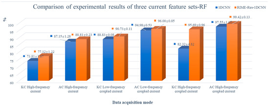
Figure 7.
Comparison of experimental results of three current feature sets.
Author Contributions
Formal analysis, S.H.; Data curation, T.K.; Writing—original draft, X.H. All authors have read and agreed to the published version of the manuscript.
Funding
This research received no external funding.
Data Availability Statement
Data are contained within the article.
Conflicts of Interest
The authors declare no conflicts of interest.
Appendix A
Table A1.
Experimental results of low frequency coupled current feature set.
Table A1.
Experimental results of low frequency coupled current feature set.
| Type | 1DCNN | Res-1DCNN | RIME-1DCNN | RIME-Res-1DCNN |
|---|---|---|---|---|
| TP | 3876 ± 11 | 3748 ± 21 | 3927 ± 12 | 3940 ± 24 |
| FP | 294 ± 12 | 105 ± 15 | 217 ± 17 | 200 ± 22 |
| FN | 111 ± 13 | 239 ± 21 | 60 ± 12 | 47 ± 23 |
| TN | 1712 ± 13 | 1901 ± 15 | 1789 ± 18 | 1806 ± 22 |
| Sp (%) | 85.34 ± 1.27 | 94.77 ± 0.73 | 89.18 ± 0.95 | 90.03 ± 0.11 |
| Se (%) | 97.22 ± 0.96 | 94.01 ± 2.56 | 98.50 ± 0.27 | 98.82 ± 0.61 |
| Ac (%) | 93.24 ± 0.77 | 94.26 ± 1.01 | 95.38 ± 0.86 | 95.88 ± 0.03 |
| KC (%) | 84.47 ± 2.55 | 87.32 ± 3.86 | 89.42 ± 0.33 | 90.57 ± 0.01 |
| KC1 (%) | 78.94 ± 1.24 | 91.86 ± 0.07 | 84.36 ± 1.25 | 85.57 ± 1.51 |
| KC2 (%) | 90.85 ± 1.37 | 83.21 ± 4.86 | 95.12 ± 1.21 | 96.19 ± 2.42 |
Table A2.
Experimental results of low frequency coupled current feature set—PCA.
Table A2.
Experimental results of low frequency coupled current feature set—PCA.
| Type | 1DCNN | Res-1DCNN | RIME-1DCNN | RIME-Res-1DCNN |
|---|---|---|---|---|
| TP | 3675 ± 24 | 3761 ± 15 | 3854 ± 22 | 3872 ± 11 |
| FP | 257 ± 17 | 320 ± 16 | 394 ± 14 | 406 ± 12 |
| FN | 312 ± 21 | 226 ± 12 | 133 ± 17 | 115 ± 11 |
| TN | 1749 ± 21 | 1686 ± 22 | 1612 ± 26 | 1600 ± 14 |
| Sp (%) | 87.19 ± 4.21 | 84.05 ± 3.53 | 80.36 ± 5.21 | 79.76 ± 2.32 |
| Se (%) | 92.17 ± 2.86 | 94.33 ± 1.93 | 96.66 ± 0.82 | 97.12 ± 1.07 |
| Ac (%) | 90.51 ± 0.75 | 90.89 ± 0.12 | 91.20 ± 0.72 | 91.31 ± 0.75 |
| KC (%) | 78.82 ± 1.27 | 79.30 ± 0.93 | 79.60 ± 0.57 | 79.75 ± 0.73 |
| KC1 (%) | 80.47 ± 4.11 | 76.57 ± 2.72 | 72.29 ± 4.76 | 71.65 ± 2.94 |
| KC2 (%) | 77.25 ± 7.12 | 82.23 ± 2.52 | 88.54 ± 2.22 | 89.92 ± 4.52 |
Table A3.
Experimental results of low frequency coupled current feature set—MIV.
Table A3.
Experimental results of low frequency coupled current feature set—MIV.
| Type | 1DCNN | Res-1DCNN | RIME-1DCNN | RIME-Res-1DCNN |
|---|---|---|---|---|
| TP | 3774 ± 11 | 3694 ± 17 | 3759 ± 11 | 3871 ± 9 |
| FP | 227 ± 15 | 290 ± 24 | 228 ± 11 | 294 ± 11 |
| FN | 291 ± 11 | 194 ± 18 | 149 ± 13 | 119 ± 12 |
| TN | 1701 ± 17 | 1815 ± 23 | 1857 ± 11 | 1709 ± 8 |
| Sp (%) | 87.51 ± 3.26 | 85.66 ± 4.07 | 81.63 ± 3.21 | 89.50 ± 4.86 |
| Se (%) | 91.36 ± 2.41 | 93.47 ± 2.61 | 95.81 ± 1.73 | 97.32 ± 2.09 |
| Ac (%) | 90.25 ± 0.47 | 90.93 ± 0.56 | 91.68 ± 1.42 | 92.07 ± 1.42 |
| KC (%) | 79.63 ± 2.08 | 79.37 ± 1.17 | 79.66 ± 0.76 | 80.30 ± 1.28 |
| KC1 (%) | 79.62 ± 3.34 | 77.53 ± 3.41 | 75.82 ± 5.38 | 73.69 ± 4.15 |
| KC2 (%) | 78.96 ± 6.12 | 81.96 ± 3.17 | 88.92 ± 1.76 | 89.71 ± 5.25 |
Table A4.
Experimental results of low frequency coupled current feature set—RF.
Table A4.
Experimental results of low frequency coupled current feature set—RF.
| Type | 1DCNN | Res-1DCNN | RIME-1DCNN | RIME-Res-1DCNN |
|---|---|---|---|---|
| TP | 3796 ± 13 | 3849 ± 11 | 3986 ± 7 | 3987 ± 11 |
| FP | 110 ± 7 | 177 ± 4 | 283 ± 3 | 240 ± 4 |
| FN | 191 ± 11 | 138 ± 13 | 1 ± 1 | 1 ± 1 |
| TN | 1896 ± 6 | 1829 ± 4 | 1723 ± 11 | 1766 ± 9 |
| Sp (%) | 94.52 ± 2.47 | 91.18 ± 0.74 | 85.89 ± 3.57 | 88.03 ± 4.13 |
| Se (%) | 95.21 ± 1.58 | 96.54 ± 2.12 | 99.97 ± 0.03 | 99.91 ± 0.09 |
| Ac (%) | 94.98 ± 0.53 | 94.74 ± 0.97 | 95.26 ± 1.22 | 96.00 ± 0.85 |
| KC (%) | 88.83 ± 0.08 | 88.14 ± 0.05 | 88.97 ± 0.77 | 90.73 ± 0.11 |
| KC1 (%) | 91.59 ± 2.82 | 86.87 ± 3.17 | 80.19 ± 6.35 | 83.04 ± 3.24 |
| KC2 (%) | 86.24 ± 3.97 | 89.45 ± 1.86 | 99.91 ± 0.07 | 99.91 ± 0.09 |
Table A5.
Experimental results of high frequency coupled current feature set.
Table A5.
Experimental results of high frequency coupled current feature set.
| Type | 1DCNN | Res-1DCNN | RIME-1DCNN | RIME-Res-1DCNN |
|---|---|---|---|---|
| TP | 3950 ± 22 | 4116 ± 37 | 4157 ± 1 | 4129 ± 53 |
| FP | 2 ± 2 | 55 ± 29 | 168 ± 2 | 10 ± 1 |
| FN | 207 ± 23 | 41 ± 39 | 2 ± 2 | 28 ± 49 |
| TN | 326 ± 2 | 273 ± 21 | 158 ± 1 | 318 ± 6 |
| Sp (%) | 99.39 ± 1.21 | 83.23 ± 8.84 | 48.17 ± 0.27 | 96.95 ± 0.31 |
| Se (%) | 95.02 ± 0.47 | 99.01 ± 0.83 | 99.91 ± 0.07 | 99.33 ± 1.30 |
| Ac (%) | 95.34 ± 0.43 | 97.86 ± 0.22 | 96.21 ± 0.08 | 99.15 ± 1.18 |
| KC (%) | 73.31 ± 1.79 | 83.89 ± 0.12 | 63.27 ± 0.04 | 93.90 ± 7.47 |
| KC1 (%) | 99.31 ± 1.36 | 81.97 ± 9.07 | 46.29 ± 0.02 | 96.70 ± 0.28 |
| KC2 (%) | 58.10 ± 2.81 | 85.91 ± 13.1 | 99.91 ± 0.08 | 91.27 ± 13.3 |
Table A6.
Experimental results of high frequency coupled current feature set—PCA.
Table A6.
Experimental results of high frequency coupled current feature set—PCA.
| Type | 1DCNN | Res-1DCNN | RIME-1DCNN | RIME-Res-1DCNN |
|---|---|---|---|---|
| TP | 3840 ± 157 | 3845 ± 141 | 3950 ± 173 | 3974 ± 180 |
| FP | 39 ± 11 | 28 ± 14 | 2 ± 1 | 6 ± 5 |
| FN | 214 ± 51 | 210 ± 11 | 207 ± 52 | 183 ± 5 |
| TN | 392 ± 193 | 402 ± 193 | 326 ± 147 | 322 ± 79 |
| Sp (%) | 97.25 ± 0.13 | 97.95 ± 0.08 | 99.39 ± 0.19 | 98.17 ± 0.27 |
| Se (%) | 94.08 ± 1.02 | 94.82 ± 1.81 | 95.02 ± 3.24 | 95.60 ± 4.35 |
| Ac (%) | 94.28 ± 1.07 | 95.03 ± 0.05 | 95.34 ± 0.07 | 95.79 ± 0.22 |
| KC (%) | 72.94 ± 0.07 | 73.19 ± 2.08 | 73.31 ± 4.35 | 75.10 ± 5.12 |
| KC1 (%) | 97.44 ± 0.84 | 98.26 ± 0.42 | 99.31 ± 0.18 | 97.94 ± 0.44 |
| KC2 (%) | 58.72 ± 11.8 | 59.27 ± 12.1 | 58.10 ± 15.4 | 60.90 ± 12.4 |
Table A7.
Experimental results of high frequency coupled current feature set—MIV.
Table A7.
Experimental results of high frequency coupled current feature set—MIV.
| Type | 1DCNN | Res-1DCNN | RIME-1DCNN | RIME-Res-1DCNN |
|---|---|---|---|---|
| TP | 4156 ± 11 | 4155 ± 21 | 4156 ± 19 | 4126 ± 12 |
| FP | 274 ± 21 | 256 ± 13 | 256 ± 11 | 241 ± 17 |
| FN | 1 ± 1 | 2 ± 2 | 1 ± 1 | 5 ± 4 |
| TN | 54 ± 19 | 71 ± 31 | 71 ± 25 | 113 ± 29 |
| Sp (%) | 16.46 ± 12.9 | 21.65 ± 11.3 | 21.65 ± 13.4 | 32.67 ± 7.28 |
| Se (%) | 99.98 ± 0.01 | 99.95 ± 0.06 | 99.98 ± 0.02 | 99.70 ± 0.18 |
| Ac (%) | 93.87 ± 3.76 | 94.23 ± 2.09 | 94.25 ± 2.76 | 94.18 ± 1.06 |
| KC (%) | 26.66 ± 9.43 | 33.64 ± 7.56 | 33.76 ± 6.27 | 37.92 ± 2.07 |
| KC1 (%) | 15.43 ± 12.1 | 20.25 ± 10.2 | 20.37 ± 9.06 | 23.19 ± 4.02 |
| KC2 (%) | 98.04 ± 1.95 | 97.05 ± 2.96 | 98.50 ± 1.51 | 99.15 ± 0.03 |
Table A8.
Experimental results of high frequency coupled current feature set—RF.
Table A8.
Experimental results of high frequency coupled current feature set—RF.
| Type | 1DCNN | Res-1DCNN | RIME-1DCNN | RIME-Res-1DCNN |
|---|---|---|---|---|
| TP | 4094 ± 11 | 4126 ± 16 | 4142 ± 7 | 4147 ± 8 |
| FP | 48 ± 24 | 43 ± 12 | 34 ± 2 | 16 ± 12 |
| FN | 63 ± 13 | 52 ± 17 | 14 ± 7 | 10 ± 7 |
| TN | 282 ± 38 | 265 ± 22 | 296 ± 2 | 312 ± 12 |
| Sp (%) | 85.67 ± 3.76 | 86.77 ± 2.09 | 89.63 ± 0.61 | 95.12 ± 3.66 |
| Se (%) | 98.49 ± 0.29 | 99.24 ± 0.07 | 99.66 ± 0.17 | 99.76 ± 0.17 |
| Ac (%) | 97.55 ± 1.07 | 98.46 ± 1.09 | 98.93 ± 0.20 | 99.42 ± 0.13 |
| KC (%) | 82.32 ± 4.82 | 87.59 ± 4.38 | 91.87 ± 1.47 | 95.69 ± 0.96 |
| KC1 (%) | 84.49 ± 3.62 | 85.26 ± 3.06 | 88.87 ± 0.67 | 94.74 ± 3.90 |
| KC2 (%) | 80.24 ± 4.07 | 85.95 ± 4.76 | 95.10 ± 2.41 | 96.65 ± 2.27 |
References
- Lee, D.; Kim, J. Empirical Modeling of Arc Faults Based on Recent Experimental Data and Field Studies. IEEE Trans. Ind. Electron. 2024, 71, 7942–7953. [Google Scholar]
- Carter, T.; Wang, J. Elmore Model-Based Analysis of High-Current Arc Faults and Their Impact on Electrical Systems. Energy Rep. 2024, 11, 1104–1118. [Google Scholar]
- Nakamura, K.; Nakajima, H. Improvement of Arc Fault Detection Based on Sato Model and Machine Learning. Electr. Power Syst. Res. 2024, 221, 107295. [Google Scholar]
- Yang, G.; Li, T.; Zhang, X. Review of Arc Fault Detection Methods and the Application of Mayr Model in Electrical Arc Fault Detection. IEEE Trans. Power Electron. 2024, 39, 5398–5410. [Google Scholar]
- Lee, S.H.; Kim, K.R. Detection of Arc Faults Using Optical Emission Analysis: Review and Advances. IEEE Trans. Power Deliv. 2022, 37, 1992–2001. [Google Scholar]
- Xu, T.W.; Liu, Z.J. Arc Fault Detection Based on Acoustic Emission Monitoring: Recent Developments and Future Directions. Sens. Actuators A Phys. 2024, 336, 113386. [Google Scholar]
- Smith, A.B.; Huang, J.L. Electromagnetic Radiation-Based Arc Fault Detection: A Review of Techniques and Applications. J. Electr. Eng. Technol. 2023, 18, 1401–1412. [Google Scholar]
- Patel, R.M.; Wang, H.J. Monitoring Environmental Temperature and Pressure Changes Induced by Electrical Arcs for Fault Detection. IEEE Trans. Ind. Electron. 2024, 71, 6297–6306. [Google Scholar]
- Kim, J.C.; Lehman, B.; Ball, R. A Series DC Arc Fault Detection Algorithm Based on PV Operating Characteristics and Detailed Extraction of Pink Noise Behavior. In Proceedings of the 2021 IEEE Applied Power Electronics Conference and Exposition (APEC), Phoenix, AZ, USA, 21–25 March 2021; pp. 989–994. [Google Scholar] [CrossRef]
- Zhao, S.; Wang, Y.; Niu, F.; Zhu, C.; Xu, Y.; Li, K. A Series DC Arc Fault Detection Method Based on Steady Pattern of High-Frequency Electromagnetic Radiation. IEEE Trans. Plasma Sci. 2019, 47, 4370–4377. [Google Scholar] [CrossRef]
- Johnson, C.D. Utilizing Optical Sensors for Arc Fault Detection in Electrical Systems. J. Electr. Eng. Technol. 2023, 19, 1025–1037. [Google Scholar]
- Brown, M.R.; Lee, H.A. Acoustic Emission Techniques for Arc Fault Detection and Diagnostics. IEEE Access 2023, 11, 15032–15044. [Google Scholar]
- Johnson, D.A. Application of Electromagnetic Sensors for Arc Fault Detection in Power Systems. Int. J. Electr. Power Energy Syst. 2024, 129, 106915. [Google Scholar]
- Smith, E.K.; Zhao, L.Y. Detecting Electrical Arcs Using Environmental Temperature and Pressure Sensors. Energy Rep. 2023, 10, 1052–1061. [Google Scholar]
- Park, S.J.; Kim, K.H. Voltage Signal Analysis for Arc Fault Detection in Low Voltage AC Systems. IEEE Trans. Power Deliv. 2021, 36, 1234–1241. [Google Scholar]
- Zhang, L.M.; Wang, Y.X. Low-Frequency Current Signal Characteristics in Series Arc Faults for Low Voltage AC Circuits. IEEE Access 2022, 10, 34567–34578. [Google Scholar]
- Lee, H.R.; Choi, J.P. High-Frequency Current Signal Analysis for Detection of Series Arc Faults in Low Voltage AC Networks. J. Electr. Eng. Technol. 2022, 17, 2310–2319. [Google Scholar]
- Liu, M.T.; Zhang, F.L. Coupled Current Signal Detection for Identifying Series Arc Faults in Low Voltage AC Systems. Int. J. Electr. Power Energy Syst. 2023, 129, 106908. [Google Scholar]
- Zhang, S.T.; Lin, J.W. Arc Fault Detection in Low Voltage Systems Using Fourier Transform and Machine Learning. IEEE Trans. Power Deliv. 2021, 36, 2309–2318. [Google Scholar]
- Wu, M.H.; Sun, L.Q. Wavelet Packet Transform-Based Feature Extraction for Arc Fault Detection in AC Circuits. Electr. Power Syst. Res. 2022, 197, 107382. [Google Scholar]
- Li, T.Y.; Zhang, Z.F. Arc Fault Detection Using Empirical Mode Decomposition and Support Vector Machines. IEEE Access 2021, 9, 68534–68543. [Google Scholar]
- Liu, Y.H.; Wang, J.K. Variational Mode Decomposition and Deep Learning for Series Arc Fault Detection in Electrical Systems. IEEE Trans. Ind. Inform. 2022, 18, 1542–1551. [Google Scholar]
- Chen, X.F.; Zhang, H.J. Complete Ensemble Empirical Mode Decomposition for Arc Fault Detection in Power Systems. J. Electr. Eng. Technol. 2023, 18, 103–112. [Google Scholar]
- Zhao, L.M.; Hu, R.T. Multi-Modal Feature Extraction and Intelligent Detection of Arc Faults Using Advanced Signal Processing Techniques. Energy Rep. 2023, 10, 1589–1602. [Google Scholar]
- Jiang, J.; Wen, Z.; Zhao, M.; Bie, Y.; Li, C.; Tan, M.; Zhang, C. Series Arc Detection and Complex Load Recognition Based on Principal Component Analysis and Support Vector Machine. IEEE Access 2019, 7, 47221–47229. [Google Scholar] [CrossRef]
- Han, C.; Wang, Z.; Tang, A.; Gao, H.; Guo, F. Recognition Method of AC Series Arc Fault Characteristics under Complicated Harmonic Conditions. IEEE Trans. Instrum. Meas. 2021, 70, 1–9. [Google Scholar] [CrossRef]
- Li, J.H.; Zhang, X.S. Application of Backpropagation Neural Network for Arc Fault Detection in Electrical Systems. J. Electr. Eng. Technol. 2022, 17, 1654–1663. [Google Scholar]
- Zhang, Y.Q.; Wang, W.J. Extreme Learning Machine for Detection of Arc Faults in Low Voltage Power Systems. IEEE Trans. Power Electron. 2022, 37, 4567–4576. [Google Scholar]
- Chen, L.Y.; Zhao, S.J. Probabilistic Neural Network-Based Arc Fault Detection in Electrical Circuits. Neurocomputing 2023, 492, 85–95. [Google Scholar]
- Liu, M.H.; Zhang, T.L. Fully Connected Neural Networks for Accurate Arc Fault Detection in Low Voltage Systems. Int. J. Electr. Power Energy Syst. 2023, 138, 108711. [Google Scholar]
- Xing, L.; Wen, Y.; Xiao, S.; Zhang, D.; Zhang, J. A Deep Learning Approach for Series DC Arc Fault Diagnosing and Real-Time Circuit Behavior Predicting. IEEE Trans. Electromagn. Compat. 2022, 64, 569–579. [Google Scholar] [CrossRef]
Disclaimer/Publisher’s Note: The statements, opinions and data contained in all publications are solely those of the individual author(s) and contributor(s) and not of MDPI and/or the editor(s). MDPI and/or the editor(s) disclaim responsibility for any injury to people or property resulting from any ideas, methods, instructions or products referred to in the content. |
© 2024 by the authors. Licensee MDPI, Basel, Switzerland. This article is an open access article distributed under the terms and conditions of the Creative Commons Attribution (CC BY) license (https://creativecommons.org/licenses/by/4.0/).