Co-Design of a Wind–Hydrogen System: The Effect of Varying Wind Turbine Types on Techno-Economic Parameters

Abstract

Green hydrogen is crucial for achieving climate neutrality and replacing fossil fuels in processes that are hard to electrify. Wind farms producing electricity and hydrogen can help mitigate stress on electricity grids and enable new markets for operators. While optimizing wind farms for electricity production is well-established, optimizing combined wind–hydrogen systems is a relatively new research field. This study examines the potential profit of wind–hydrogen systems by conducting a case study of an onshore wind farm near the North Sea. Varying turbine types from high wind-speed turbines (with high annual energy production) to low wind-speed turbines (with high full-load hours) are examined. Findings indicate that in a combined hydrogen system, the low wind-speed turbines, which are sub-optimal for mere electricity production, yield lower levelized costs of hydrogen at a higher hydrogen production. Although high wind-speed turbines generate higher profits under current market conditions, at high hydrogen prices and low electricity prices, low wind-speed turbines can yield higher total profit at this site. Therefore, an integrated optimization approach of wind–hydrogen systems can, in certain cases, lead to better results compared to an isolated, sequential optimization of each individual system.

1. Introduction

Green hydrogen is a crucial component in the transition towards a 100% sustainable energy system, as it can replace fossil fuels in processes that are challenging to electrify, such as crude steel production [1]. In order to meet the growing demand for green hydrogen, the European Commission has set a target of 10 million tons of green hydrogen to be produced annually within the European Union by 2030 [2]. This is equivalent to an installed electrolyzer capacity of approximately 100 GW, which will require substantial quantities of Renewable Energy Sources (RESs) [3]. The production of green hydrogen from wind energy can improve the utilization of Wind Farms (WFs), while mitigating bottlenecks in the electricity grid that otherwise result in wind energy curtailment. The construction of electrolyzers, in combination with WFs, offers new opportunities for WF developers and operators, in addition to the mere sale of electricity. However, this also poses new challenges regarding the design of wind–hydrogen systems, which are referred to as hybrid wind farms in this study. Consequently, hybrid WFs present an emerging field of research and business development [4].

The optimization of WFs for electricity production is a well-established research area. The objective of conventional methods is typically to design an optimal layout, with the goal of minimizing the Levelized Cost Of Electricity (LCOE) while maximizing the Annual Energy Product (AEP) to enhance the WF profitability [5,6]. This includes selecting the most suitable Wind Turbine Generator (WTG), determining the optimal WTG positions, and choosing the hub height (H) and rotor diameter (RD). However, the design process of wind–hydrogen systems presents a challenge in determining the optimal design criteria for the combined system of the WF and the hydrogen-producing system components. One approach is to initially design the WF layout and select WTGs based on the LCOE and AEP optimization and sequentially optimize the hydrogen system. However, it is unclear, if this approach will result in the overall most profitable hybrid WF. This is particularly the case in scenarios where enhancing the efficiency of the hydrogen system by varying WF design parameters from their optimum leads to a decrease in the efficiency of the WF. It should therefore be investigated, if the optimal wind–hydrogen system design requires integrating the optimization of both the WF and the hydrogen system.

Numerous studies on the optimal design of wind–hydrogen systems have been conducted. While addressing various different aspects, the most common objective is to reduce the Levelized Cost Of Hydrogen (LCOH).

Hofrichter et al. [7] consider different locations that are characterized by varying full load hours (FLHs) of a WF. They vary the installed wind power at these locations and determine the optimal ratio between rated power of the electrolyzer and the WF, to achieve minimal LCOH (LCOH_min). The steps in the variation of installed wind power are arbitrary between 0.5 and 50 MW, with a fixed hub height H of 150 m for the considered WTGs. In their study, Grant et al. [8] determine the LCOH that can be achieved for a fixed rated electrolyzer power (P_Ely) of 1 GW, which is fed by a hybrid power plant containing photovoltaic (PV) plants and WTGs. The authors generate results for over 50,000 locations in the USA with various combined WF and PV plant capacities. They utilize six MW reference WTGs, each with a fixed hub height H of 140 m, to calculate the power generation profile of the WF on site. Ibagon et al. [9] first specify a quantity of hydrogen to be produced and the dimension of the renewable capacity of the WF and PV plants accordingly, in order to achieve LCOH_min. Although the generation capacity is used on a site-specific and hourly basis, no detailed information on the WTGs used is provided.

While the installed capacity of the RES at a given location varies across these studies, the selected WTGs, their hub height H and RD or rated power (P_WTG) remain constant within each study. Additionally, the WF itself is not subjected to a comprehensive analysis, as no optimization of the WFs is conducted [7,8,9]. For example, all studies assume that the available area is suitable for installing additional WTGs when required to achieve LCOH_min. Schnuelle et al. [10] consider different WFs with different turbine types in their study of hydrogen production costs from dynamic wind and PV. However, they do not vary the turbine types at a specific site, as their focus is on optimizing the electrolyzer operating strategies, not on optimizing the WF, which is treated as a fixed input. Additionally, there are numerous studies, such as [11,12], on ideal sites on a continental or regional scale for hydrogen production from wind or PV, but as they take a macroscopic approach, they also do not vary the WTGs used.

In a previous study, we conducted a case study in which the WTGs used in a WF were varied and the effects on the resulting LCOH were discussed. It was assumed that the electrolyzer is only fed by electricity provided by the WF. Thus, the electricity cost was set as equal to the LCOE of the WF. Nevertheless, despite the variation in AEP and the Load Duration Curve (LDC) based on the WTG variation, the assumption was made that LCOE would remain constant [13]. However, the LCOE is highly dependent on FLHs and capital expenditures (CAPEX) for the WTGs [14]. Additionally, the effect of varying WTGs with fixed positions on the LDC has been simplified, as wake effects were neglected.

Several studies have shown that the LCOH of wind–hydrogen systems is driven by the electricity costs and the capacity utilization of the electrolyzer, in addition to the high investment costs of electrolyzers [8,9,13,15,16]. However, the impact of changes in WF design parameters, such as the selection of different WTGs, have not been adequately addressed in the literature. The aim of this paper is to demonstrate that there are interdependencies between the WF and the hydrogen system that necessitate an integrated optimization of both system designs. Therefore, a tool chain is established that combines a bottom-up WTG cost model [17,18], a WF optimizer [5], and a wind–hydrogen system optimization model [13]. A description of the models used and their interactions is provided in Section 2. This novel tool chain is then applied to analyze the impact of different WTGs on various key performance indicators, including the LCOE, LCOH and AEP of the wind–hydrogen system for a selected case study in northern Germany. Section 3 presents a description of the WF site on the German North Sea coast that was used for this case study, and the corresponding results. The results, model limitations, and implications for future research are finally discussed in Section 4. A complete list of abbreviations used throughout this study is provided in

Table A1. Complete list of abbreviations used throughout this document.

Abbreviation		Abbreviation
AEL	Alkaline Electrolyzer	POD	Point Of Demand
AEP	Annual Energy Product	PV	Photovoltaic
AHP	Annual Hydrogen Product	PWF	rated WF Power
AP	Annual Profit	PWTG	rated Wind Turbine Generator Power
CAPEX	Capital Expenditures	RD	Rotor Diameter
cComponent	Component Cost	RES	Renewable Energy Sources
CFEly	Capacity Utilization Electrolyzer	TOTEX	Total Expenditures
ECHS	Electricity Consumption Hydrogen System	vcutin	cut in wind speed
FLH	Full-Load Hours	vcutout	cut out wind speed
H	Hub Height	WF	Wind Farm
HyDe	Hybrid Wind Farm Design Environment	WIFO	Wind Farm Optimizer
LCOE	Levelized Cost Of Electricity	WTG	Wind Turbine Generator
LCOH	Levelized Cost Of Hydrogen	5MW100	5 MW WTG with 100 m H
LDC	Load Duration Curve	5MW120	5 MW WTG with 120 m H
LROE	Levelized Revenue Of Electricity	5MW140	5 MW WTG with 140 m H
LROH	Levelized Revenue Of Hydrogen	7MW140	7 MW WTG with 140 m H
OPEX	Operational Expenditures	WF5MW100	WF with 5 MW WTG with 100 m H
PEl/PWF	ratio PEly to PWF	WF5MW120	WF with 5 MW WTG with 120 m H
PEly	rated Electrolyzer Power	WF5MW140	WF with 5 MW WTG with 140 m H
PEMEL	Proton Exchange Membrane Electrolyzer	WF7MW140	WF with 7 MW WTG with 140 m H
POCC	Point Of Common Coupling

.

2. Materials and Methods

The following section provides an overview of the utilized WTG cost model, the WF optimizer, the wind–hydrogen system optimization model, and their combinations in a novel tool chain. Additionally, model assumptions and adaptions are presented.

It is assumed that the electrolyzer in this study is operated exclusively with electricity generated by the WF, while no additional grid electricity is used. The surplus electricity produced by the WF, which is not consumed by the electrolyzer, is fed into the electricity transmission grid. A schematic overview of the models and their interactions is illustrated in Figure 1. In this study, the WF optimization environment is referred to as Wind Farm Optimizer (WIFO) [5], and the wind–hydrogen system optimization model developed by Reichartz et al. [13] is referred to as Hybrid Wind Farm Design Environment (HyDE). The input data, indicated in green, can be classified into three categories: WTG data such as hub height H or rotor diameter RD, WF site-specific data such as wind data, and WF layout and market data, such as electricity or hydrogen price. For this study, the assumption is made that the electricity price p_el and hydrogen price p_H2 are constant over time and therefore equal the Levelized Revenue Of Electricity (LROE) and Levelized Revenue Of Hydrogen (LROH), respectively. The design parameters that are varied in this study are turbine power P_WTG (varying between 5 MW and 7 MW), hub height H (varying in the range of 100 m to 140 m), and rotor diameter RD (varying between 162 and 185 m). The three central calculation models of the toolchain presented are described in the following.

2.1. WTG Cost Model

The LCOE of a WF depend, among other factors, on the total expenditures (TOTEX), which in turn depend largely on the CAPEX for the selected WTGs, transportation, installation and balance of plant [6]. The costs for a WTG (CAPEX_WTG) are dependent on a number of factors, including the rated-power P_WTG, the rotor diameter RD, and the hub height H [17,19]. To calculate the CAPEX_WTG for different WTGs, the cost model proposed by Reichartz et al. [17,18] is utilized. One advantage of this method is that the costs for the most expensive WTG components, such as the tower (c_Tower), rotor (c_Rotor), and gearbox (c_Gearbox), are determined using a bottom-up approach. This allows for differentiation between low wind-speed and high wind-speed WTGs, which usually differ significantly in RD and H [20]. Conventional top-down cost models, which only scale the costs based on the rated WTG power P_WTG, are unable to provide this differentiation. The cost model requires a minimum of three input parameters: the rated-power P_WTG, the hub height H, and the rotor diameter RD, as shown in Figure 1. However, as no further differentiations regarding CAPEX_WTG are made in this study, such as varying between WTGs with a gearbox or direct drive turbines, no additional input data are provided or varied. For a comprehensive model description, including all underlying assumptions and model equations, please refer to [17,18].

In order to calculate the WTG-dependent LCOE for a WF site (CAPEX_WF), the calculated CAPEX_WTG from the cost model is transferred into a wind farm optimizer for further calculations.

2.2. Wind Farm Optimizer (WIFO)

WIFO is a state-of-the-art WF optimizer initially designed by Roscher [5] and maintained by the Chair for Wind Power Drives at RWTH Aachen University. In this study, WIFO is utilized to calculate the LCOE for various WF configurations. These calculations are based on the AEP, CAPEX, and the operational expenditures (OPEX). The latter are currently calculated by WIFO, based on literature values. CAPEX beyond turbine cost are assumed to be EUR 521/kW (CAPEX_BOP). These consist of costs for installation, transportation, project development, and balance of plant (BOP) [21]. OPEX are calculated with a power specific component of EUR 20/kW and an energy specific component of EUR 0.008/kWh [22]. WIFO accounts for energy yield losses due to wake effects and technical turbine availability, as well as additional efficiency losses within the WF and WTGs. It is assumed that the turbine downtime is distributed evenly over each year. While alternative wake modeling methods are available, in this study the wake model proposed by Katic and Jensen is used [23]. Input data for WIFO are WTG-specific information, including CAPEX_WTG derived from the WTG cost model, rotor diameter RD, hub height H, and rated-power P_WTG. Furthermore, the cut-in wind speed v_cutin and the cut-out wind speed v_cutout of the WTGs are required input data, as the power curves of the WTGs are calculated based on this information. Additionally, WIFO requires location-specific data, such as the WF layout and wind distribution data. Based on this information, the LDC of a given WF is then derived.

The results of WIFO, including LCOE and the LDC, serve as an input for the optimization of the hydrogen-system carried out in HyDE.

As the name implies, WIFO is designed to perform optimizations of WFs for a particular site, including the WTG layout optimization. However, in this study, it is used solely for the assessment of a given WF layout with varying WTGs. The long-term objective is to integrate the WF optimization and the optimization conducted in HyDE, which is explained below. This is discussed in further detail in Section 3 and Section 4.

2.3. Hybrid Wind-Farm Design Environment (HyDE)

HyDE is an optimization tool designed to achieve LCOH_min by optimizing the hydrogen system for an existing WF with given LCOE at a specific site [13]. In HyDE, only proton exchange membrane electrolyzers (PEMELs) are considered, as they are more suitable for on-site hydrogen production with WFs than alkaline electrolyzers (AELs). This is due to several factors, including better load flexibility and shorter cold and warm start times, compared to AELs [24,25,26,27]. To calculate the optimal ratio for LCOH_min between electrolyzer power P_Ely and rated WF power P_WF (P_Ely/P_WF), the capacity utilization of the electrolyzer (CF_Ely) is calculated as dependent on P_Ely. The CF_Ely is defined as the fraction of hours per year during which the electrolyzer is operated at equivalent rated power P_Ely [13], while the rated WF power P_WF is the sum of P_WTG of all turbines in the farm. The calculation of CF_Ely is based on the LDC provided by WIFO. Additionally, the logistics of hydrogen transportation to the Point Of Demand (POD) are considered. HyDE automatically identifies the optimal distribution mode and carries out the necessary calculations for the sizing of the required infrastructure for the supply of hydrogen from the WF site to the POD. The LCOHs calculated by HyDE therefore already include hydrogen transportation costs. The distribution modes considered include a variety of tractor and trailer combinations and hydrogen transportation via pipeline. The original source provides a comprehensive overview of the model assumptions, including a detailed cost breakdown for all components and the relevant equations [13].

In order to perform the optimization, additional input parameters regarding the WF site are required. These include the Point Of Common Coupling (POCC) of the WF, as it is assumed that the electrolyzer is connected to the internal electricity grid of the WF. As the electrolyzer requires water, it is necessary to define the nearest suitable water supply point. Additionally, the POD and the position of the electrolyzer must also be defined. HyDE is capable of optimizing the electrolyzer position on the WF site. However, this feature is not used in the present study, as only a fixed electrolyzer position is considered.

The initial HyDE model discussed in [13] has been modified and improved as follows: in [13], it is assumed that the electrolyzer has a constant efficiency, regardless of the power it is currently operating at. Given the particularly poor partial-load performance of PEMEL at low power, it is assumed that the electrolyzer is shut down if the WF power output is less than 10% of P_Ely in this study. This is in line with other research [28,29]. An operation of the electrolyzer in overload (>100% of P_Ely) is not considered. In accordance with [13], it is assumed that the efficiency of the electrolyzer is constant for the remaining load range.

As previously stated, HyDE is intended to achieve LCOH_min for a wind–hydrogen system. However, WFs that solely produce electricity are typically designed to generate maximum profits over their lifetime, and not only for a minimal LCOE [30]. This requires knowledge about the achievable revenue for electricity over the lifetime of the WFs. Therefore, in order to optimize the wind–hydrogen system, which produces hydrogen and electricity, for maximum profit, additional knowledge about the achievable revenue for hydrogen is necessary.

To optimize the wind–hydrogen system for profit, HyDE is extended by incorporating Equation (1). The annual profit (AP, in EUR/a) is calculated as a function of the rated electrolyzer power P_Ely. Therefore, the electricity consumption of the hydrogen system (ECHS, in kWh/a), which includes not only the electricity usage of the PEMEL, but also that of auxiliary infrastructure such as pumps, is determined based on P_Ely and its corresponding CF_Ely. To calculate the AP, additionally the Levelized Revenue Of Electricity (LROE, in EUR/kWh) and the Levelized Revenue Of Hydrogen (LROH, in EUR/kWh) is used. In contrast to LCOE, LROE does not quantify the cost of electricity, but it assesses the revenue generated from electricity sales [31]. The same concept is applied here to hydrogen, for LROH. AHP is the Annual Hydrogen Product (in kWh/a) of the wind–hydrogen system.

AP = (AEP − ECHS) × (LROE − LCOE) + AHP × (LROH − LCOH)

(1)

Therefore, additional market data inputs are required, including electricity prices p_el and hydrogen prices p_H2, as shown in Figure 1. As a simplified assumption, LROHs are set equal to p_H2 and LROEs are set equal to p_el.

The tool chain, which comprises the WTG cost model, WIFO, and the modified HyDE version, is used to generate results for a WF site with varying WTGs. This analysis aims to determine the preferable hybrid farm design, based on overall profit from both electricity and hydrogen production, and to evaluate key performance indicators such as LCOE, LCOH, and AP.

The authors acknowledge that ChatGPT, and DeepL were used to assist with formulating some of the text in this work [32,33].

3. Results

This section first describes the WF site and the WTGs under consideration. Necessary input data, including those required for the analysis of the hydrogen system, are provided. In addition, the results of the sub-models, the WTG cost model, WIFO and HyDE are presented.

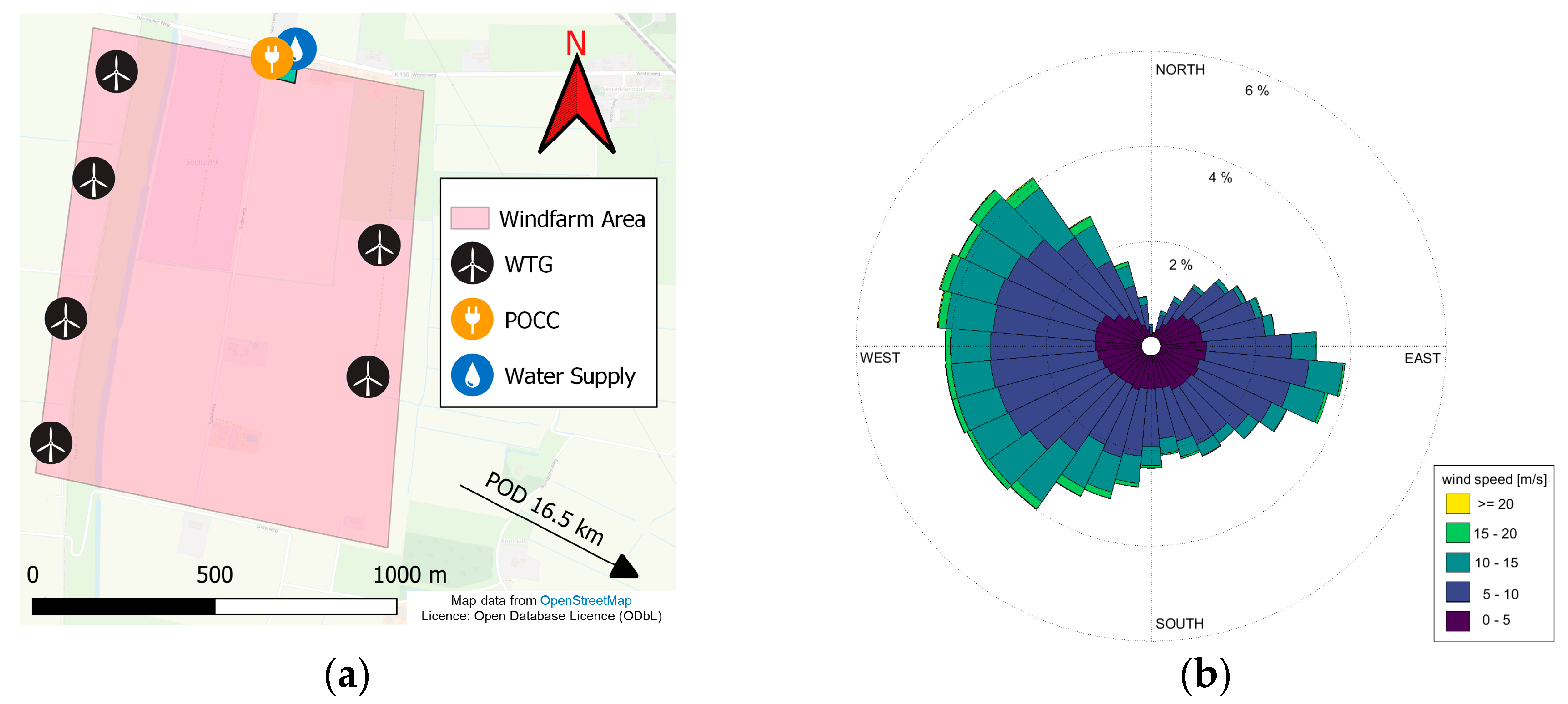
3.1. Wind Farm Site and Wind Turbine Generators

The WF site is located approximately 3 km east of the North Sea coastline in the municipality Friedrich-Wilhelm-Lübke-Koog in Germany. The area is part of an existing WF illustrated schematically in Figure 2a. In total, the WF consists of six WTGs, positioned as shown below. Figure 2b displays the wind rose for the site at an elevation of 80 m above ground level. The cumulated Weibull scale parameter is 9.24, with a shape parameter of 2.35. The meteorological data of the WF site are derived from historical hourly wind measurements obtained from measurement stations operated by Deutscher Wetterdienst [34].

It is assumed that the water supply for the electrolyzer is located in the close vicinity of the WF site, in proximity to the POCC of the WF. As illustrated in Figure 2a, the POD is located approximately 16.5 km to the southeast of the WF site. The POD is a hydrogen pipeline that is part of the German hydrogen core network. Although the network is not yet operational, its construction has been proposed for 2024 by a consortium of gas transmission system operators [35]. The gas transmission grid is assumed to have a capacity that is significantly greater than the hydrogen production capacity of a single WF. Consequently, it is assumed that all hydrogen produced can be sold without further limitations. This assumption is also reflected in the expectation that the German hydrogen demand cannot be fully met, at least in the short and medium term [3].

While the WTG positions remain constant throughout this study, the WTG types are varied. The technical specifications of the WTGs considered are listed in

Table 1. Technical specifications of considered WTGs and resulting CAPEX_WTG.

Parameter	5 MW WTG	7 MW WTG
PWTG (MW)	5	7
RD (m)	185	162
H (m)	100/120/140	140
Power density (W/m2)	186	340
vcutin (m/s)	3	3
vcutout (m/s)	22	25
CAPEXWTG (€/kW) 1	1251/1274/1297	931

¹ as calculated by the WTG cost model [17,18].

. The turbine specifications used here are artificial, yet they are based on existing WTGs. Two different WTG types are considered, one typical low wind-speed WTG with a RD of 185 m and a rated power P_WTG of 5 MW, and one typical high wind-speed WTG with a RD of 162 m and P_WTG of 7 MW. It is assumed that the low wind-speed 5 MW WTG has a lower cut-out wind speed v_cutout than the 7 MW turbine. Both WTGs have the same cut-in wind speed v_cutin. Three different hub heights H are considered for the 5 MW WTG. Therefore, a total of four turbine configurations, and thus four different WF configurations are analyzed. To increase readability, the 5 MW turbine with a hub height of 100 m will be referred to in the following as 5MW100, the 5 MW turbine with a hub height of 120 m as 5MW120, and so forth. It should be noted at this point that a hub height of 100 m is unusually low for a turbine with an RD of 185 m, but is included here as a lower-bound estimate. The power curves of the WTGs are illustrated in Figure 3a. No differentiation is made between the power curves with regard to the hub height H in this context. The power curves are calculated by WIFO [5], based on the turbine specifications given in Table 1.

CAPEX_WTG are calculated using the WTG cost model [17,18]. For better comparability, the power-specific CAPEX (in EUR/kW) are shown in Table 1. As a result of the higher RD and lower P_WTG, the power-specific CAPEX of the 5MW100, 5MW120 and 5MW140 WTGs are significantly higher than those of the 7MW140 WTG. Due to the larger tower, the power-specific CAPEX for the 5MW140 turbine is higher than for the 5 MW turbines with lower hub heights. There are no additional cost variations considered for the different WTGs. It is assumed that the WTG availability is 97% for all turbines, while the WF lifetime is assumed to be 25 years.

3.2. WIFO Results

In the following Section, the WIFO results for the previously introduced WF (see Figure 2) are presented. An overview of the results is given in

Table 2. WIFO results for the 30 MW and 42 MW WF configurations. The optimal values for CAPEX, AEP, FLH, and LCOE are highlighted in bold.

Parameter	30 MW WF	42 MW WF
WTG	5MW100/5MW120/5MW140	7MW140
CAPEXWF (Mio. €)	53.16/53.85/54.53	60.98
AEP (GW)	171.28/178.36/181.49	216.57
FLH (h)	5709/5945/6050	5157
LCOE (€ct./kWh)	3.62/3.56/3.54	3.55

. The four WF configurations with differing WTGs are referenced with WF7MW140 for the WF with the 7MW140 WTGs, and so forth. Figure 3b illustrates the calculated LDCs based on the turbine power curves and the site-specific wind distribution (see Figure 2b and Figure 3a). As evident in Figure 3b, the AEP of the WF7MW140, which is represented by the area below the dash-dotted line, is larger than that of each other turbine choice at this site. This is also shown in Table 2. The CAPEX_WF for the WF5MW100 and WF5MW120 are the lowest among the considered farm configurations. Nevertheless, the LCOEs for these two farms are the highest, at EUR 0.0362 and 0.0356/kWh, respectively. This is due to the CAPEX_WF being comparably high to that of the WF7MW140. For example, the CAPEX_WF of the WF5MW100 is only 12.8% lower than that of the WF7MW140, while the AEP is 21% lower. Although the power-specific CAPEX_WTG of the 5MW140 are the highest of all turbines (see Table 1), the LCOEs for the WF5MW140 are the lowest of all farms, yet the AEP is still 16.2% smaller than for the WF7MW140. This is a result of the lower absolute CAPEX_WF of the WF5MW140.

For the exclusive production of electricity, the WF configuration with six 7 MW high-wind speed turbines is the optimal solution for the analyzed site. This configuration yields the highest AEP at a lower (compared to the WF5MW100 and WF5MW120) or nearly identical LCOE (compared to the WF5MW140) with respect to all farm configurations with 5 MW low-wind speed turbines. In the following analysis of the farm configurations, it is investigated whether the optimal WF for electricity production is also optimal for hydrogen production. Therefore, the WIFO results (the LCOE and LDCs of all WF configurations) are put into the wind–hydrogen optimizer HyDE.

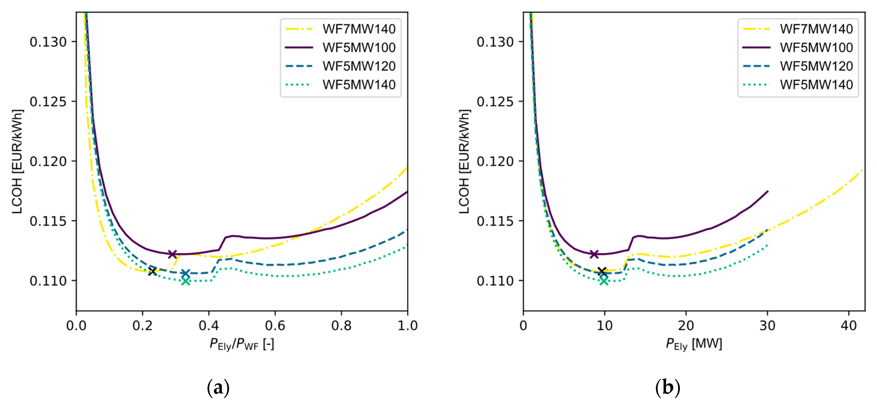
3.3. Wind–Hydrogen System

In HyDE, the electrolyzer and auxiliary infrastructure is optimized for each of the four considered WF configurations. The following section presents the impact of varying WF configurations on the design parameters and key performance indicators of the wind–hydrogen system, specifically the AHP and LCOH_min. In all calculations, the efficiency of the PEMEL is assumed to be 65%, independent of the current capacity utilization (see Section 2.3). All other parameters and cost assumptions for the PEMEL and the infrastructure necessary for the hydrogen system are based on the specifications given in [13].

Figure 4a shows the CF_Ely as a function of P_Ely/P_WF for the different WF configurations. The CF_Ely is calculated by HyDE based on the LDC derived from WIFO. While the CF_Ely does decline with an increasing P_Ely/P_WF ratio, for all WF configurations, the decline is most significant for the WF7MW140. This is due to the fact that the 7 MW WTG generates less power at lower wind speeds, relative to its rated power, than the 5 MW WTG (see Figure 3a), as it is designed for a higher rated wind speed. Consequently, since the electrolyzer is only fed from electricity generated by the WF, the CF_Ely is the lowest for the WF7MW140 for all P_Ely/P_WF. Figure 4b shows the same values over the absolute rated power of the electrolyzer P_Ely. The CF_Ely of the WF7MW140 is always higher than for the WF5MW100, regardless of P_Ely. For P_Ely values above about 6 MW, the CF_Ely of the WF5MW120 and WF5MW140 are higher than for WF7MW140. No P_Ely/P_WF ratios higher than 1 are considered.

Figure 5a shows the LCOH as a function of P_Ely/P_WF for all WF configurations. The resulting LCOH_min for each WF configuration is indicated with an X. In comparison, Figure 5b shows the same values, but again over the absolute rated power of the electrolyzer P_Ely. The results are generated by HyDE, utilizing the LDCs and LCOE calculated by WIFO and presented in Section 3.2. Additional results are shown in

Table 3. HyDE results for the different WF configurations with a hydrogen system. The optimal values for LCOH, P_Ely, CF_Ely, P_Ely/P_WF, CAPEX_Ely, and AHP are highlighted in bold.

Parameter	30 MW WF	42 MW WF
WTG	5MW100/5MW120/5MW140	7MW140
LCOHmin (€ct./kWh)	11.22/11.06/11.00	11.08
PEly (kW) 1	8700/9900/9900	9660
CFEly (%) 1	84.3/84.3/84.8	83.8
PEly/PWF (%) 1	29/33/33	23
Distribution mode 1	Diesel-LOHC 2	Diesel-LOHC 2
CAPEXEly (Mio. €) 1,3	14.04/15.76/15.78	15.40
AHP (t/a) 1	1254/1425/1436	1384

¹ values at LCOH_min. ² Diesel tractor, liquid oxygen hydrogen carrier (LOHC) trailer combination (please refer to [13] for additional information). ³ CAPEX for the additional hydrogen system, not including the CAPEX_WF of the WF.

.

As shown in Figure 5 and Table 3, the achievable LCOH_min for the WF5MW120 and WF5MW140 are lower than for the WF7MW140. However, the WF5MW100 results in the highest LCOH_min of all WF and electrolyzer configurations. The P_Ely/P_WF values at which LCOH_min are achieved are significantly higher for all WF configurations with 5 MW turbines, than for the WF configuration with the 7 MW turbine. This is a consequence of the faster declining CF_Ely for the WF7MW140, as previously described. Given that the optimal P_Ely/P_WF with regards to LCOH_min is considerably larger for the WF5MW120 and WF5MW140, it follows that the absolute electrolyzer power P_Ely is also slightly greater than for the WF7MW140 for achieving LCOH_min. Consequently, due to the higher CF_Ely and P_Ely, the WF5MW120 and WF5MW140 also lead to a greater AHP than the WF7MW140 at P_Ely/P_WF for LCOH_min (see Table 3).

In addition to the results for LCOH_min, Figure 5a,b illustrate further trends. The qualitative progression of LCOH as a function of P_Ely/P_WF or P_Ely is similar across all of the considered WF configurations. When P_Ely/P_WF is 0.1 or lower, the LCOHs are high, even though the CF_Ely is high at these ratios. The high LCOHs are a result of small electrolyzer powers P_Ely, leading to only a small AHP. Despite the low P_Ely, fixed infrastructure costs such as roads and electric cables persist, which lead to a high LCOH, due to a bad capacity utilization of the auxiliary infrastructure.

Figure 5a also shows that the LCOHs for the WF7MW140 increase significantly at P_Ely/P_WF of about 0.2, while the LCOHs for the other WF configurations show the same increase at P_Ely/P_WF of about 0.4. This is due to limited amount of hydrogen that can be transported to the POD by a single tractor–trailer combination. Therefore, the need for a second tractor and trailer increases the LCOH significantly. Since the AHP is higher for the same P_Ely/P_WF for the WF7MW140, this occurs at lower P_Ely/P_WF. However, after the increase, the LCOH start to decrease again at higher P_Ely/P_WF. This is due to the fact that the utilization of the tractor–trailer combination increases again at higher P_Ely/P_WF. These phenomena do not reappear for even higher P_Ely/P_WF, as pipeline transport becomes the most cost-effective option for AHP above a certain threshold and the costs for a pipeline do not show such discontinuities. For more information, see [13]. However, the decrease in CF_Ely with increasing P_Ely/P_WF ultimately leads to LCOH rising for higher P_Ely/P_WF. This trend is particularly evident for the WF7MW140.

Although the WF configuration with six 7 MW high-wind speed turbines is optimal for electricity production (see Section 3.2), it does not result in the lowest LCOH_min. Instead, the lowest LCOH_min at the considered site are achieved by the WF configurations with the 5 MW low-wind speed turbines (WF5MW120 and WF5MW140). However, the total energy production, which equals the AEP of the WF configurations, remains the highest for the WF7MW140. Consequently, it is unclear whether the WF configurations for optimal LCOH can outperform the WF7MW140 in profitability, considering the sale of both electricity and hydrogen. A detailed analysis, comparing the best WF configuration with low wind-speed turbines (WF5MW140) with the WF configuration with high wind-speed turbines (WF7MW140) is provided in the following Section.

3.4. Wind–Hydrogen System under Market Conditions

In Section 3.3, the HyDE results regarding the optimal P_Ely/P_WF for LCOH_min were presented. Typically, WFs that produce only electricity are designed to maximize profit over their operational lifetime, as discussed in Section 2.3. Assuming this design principle will remain consistent for hybrid WFs, these will also be optimized for maximum profitability. Consequently, the optimal P_Ely/P_WF ratio for achieving LCOH_min may not align with the optimal P_Ely/P_WF ratio for maximum annual profit (AP_max).

3.4.1. Effect of Varying LROH on the Optimal System Design

In order to design a wind–hydrogen system for AP_max, it is necessary to know the achievable LROE and LROH. Since the WF under consideration is located in Germany, the reference value for wind energy of the Erneuerbare Energien Gesetz (EEG) is used as reference LROE, which is EUR 0.0735/kWh in 2024 [36]. For simplicity, no quality correction factor is included for both WF configurations.

Figure 6a shows the AP as a function of P_Ely/P_WF for the WF5MW140, which is calculated based on Equation (1). The LROHs are varied between EUR 0.165 and 0.175/kWh here, while the LROEs of EUR 0.0735/kWh are assumed. The black horizontal line indicates the reference AP, which is achieved when no hydrogen system is installed (AHP = 0) and the entire generated electricity is sold. The vertical dashed grey line is the P_Ely/P_WF ratio for which LCOH_min are achieved (see Table 3). Figure 6b illustrates the AP for the WF7MW140, with the LROE fixed at EUR 0.0735/kWh, as in Figure 6a. The AP for the WF7MW140 is consistently higher than that for the WF5MW140 across all LROH values considered, as well as for the case with no hydrogen production (about EUR 1.5 million/a higher in this case). This is primarily due to the significantly greater AEP of the WF7MW140 (see Table 2), which results in a higher overall profit.

At an LROH of EUR 0.165/kWh, the AP_max for the WF5MW140 is higher than in the scenario of no hydrogen production. In contrast, at the same LROH, integrating an electrolyzer does not yield any advantages in terms of AP for the WF7MW140. This disparity is a result of the higher LCOH of the WF7MW140, as shown in Figure 5a,b.

The increase in LCOH at the P_Ely/P_WF values mentioned in Section 3.3, which is a consequence of the need for a second tractor and trailer, is represented here as a decline in the AP. Furthermore, the decline in AP is considerably higher for the WF7MW140 than for the WF5MW140 at higher P_Ely/P_WF values, again a result of the faster decrease in CF_Ely for the WF7MW140 compared to the WF5MW140 (see Figure 4a).

In addition, for both WFs and almost all LROH levels, there is a notable difference between the P_Ely/P_WF value that optimizes AP_max and those that result in LCOH_min. Figure 6a,b show that the P_Ely/P_WF value that maximizes the AP is sensitive to variations in LROH. For instance, while the AP remains negative compared to the AP for no hydrogen production, at an LROH of EUR 0.165/kWh for both WFs, the optimal P_Ely/P_WF ratio for maximizing the AP reaches 0.67 at an LROH of EUR 0.17/kWh for the WF5MW140. Although this trend is less distinct for the WF7MW140, it is still evident as the P_Ely/P_WF value for AP_max exceeds 0.5 at an LROH of EUR 0.175/kW, while the P_Ely/P_WF for LCOH_min is only 0.23. However, due to the trends in CF_Ely and consequently the LCOH at higher P_Ely/P_WF values, this trend is less significant.

3.4.2. Effect of Varying WTGs on the Most Profitable Hybrid WF

In the previous analysis, the effects of varying LROH on the AP and the optimal P_Ely/P_WF value for both the WF5MW140 and WF7MW140 at a fixed LROE were discussed. However, as shown in Section 3.3, the WF5MW140 outperforms the WF7MW140 in terms of achievable LCOH_min (see Table 3). The question arises, whether there is a parameter range of LROE and LROH, where the WF5MW140 also outperforms the WF7WM140 in terms of AP. Therefore, Figure 7a,b show a parameter range variation of LROE and LROH. The parameter range where the AP of the WF5MW140 exceeds the AP of the WF7MW140 is shown in green, and vice versa in blue. The results are based on Equation (1). In Figure 7a, the results are plotted for the P_Ely/P_WF values of both WFs at those that result in LCOH_min. Thus, the electrolyzer of the WF5MW140 has a rated power P_Ely of 9.9 MW, while the electrolyzer of the WF7MW140 has a rated power P_Ely of 9.66 MW (see Table 3). Since the WF5MW140 produces more hydrogen at lower cost, the AP exceeds that of the WF7MW140 at low LROE combined with high LROH. Figure 7b shows the same plot, but both electrolyzers have a rated power of 20 MW. Since the WF5MW140 performs better in terms of LCOH at higher P_Ely/P_WF values, the parameter range where the AP of the WF5MW140 exceeds the AP of the WF7MW140 shifts to higher LROE and lower LCOH.

For both electrolyzers with a rated power of 20 MW, Equation (2) defines the LROH-threshold at which the AP of the WF5MW140 exceeds that of the WF7MW140 as a function of the LROE, and thus describes the black line in Figure 7b.

LROH = 12.97 × LROE − EUR 0.397/kW

(2)

For LROH values above this linear equation, the AP of the WF5MW140 is greater, even though the WF7MW140 achieves a significantly higher AEP at the same site (see Table 2). For example, for LROE of EUR 0.05/kWh this tipping point occurs at LROH of about EUR 0.25/kWh.

3.4.3. Effect of Varying LROE on the Optimal System Design

To further investigate the effect of varying LROE on the optimal P_Ely/P_WF value for AP_max, Figure 8 presents the AP of the WF5MW140 for LROE of EUR 0.0635/kWh. Compared to the outcomes for LROE of EUR 0.0735/kWh, the AP with no hydrogen production is reduced by approximately EUR 1.8 million/a. While the addition of a hydrogen system to the WF resulted in a decrease in AP across all P_Ely/P_WF values (as shown in Figure 6a), the hydrogen system now has a positive impact on the AP at the same LROH of EUR 0.165/kWh, with the reduced LROE. Even with a reduction in LROH by EUR 0.01/kWh to EUR 0.155/kWh, the hydrogen system enhances the AP. Thus, the optimal P_Ely/P_WF value is sensitive not only to variations in LROH, but also to changes in LROE.

4. Summary and Discussion

The objective of this study was to determine whether the optimal Wind Farm (WF) design for electricity production differs from that optimized for combined electricity and hydrogen production, especially when considering different Wind Turbine Generators (WTGs). Therefore, the influence of varying WTGs in a WF on the optimal electrolyzer power P_Ely for minimal LCOH (LCOH_min) and maximum profitability (AP_max) has been investigated. A combination of pre-existing calculation models into a novel tool chain consisting of a bottom-up cost model for WTGs, a WF optimizer, and a wind–hydrogen system optimizer has been introduced.

A detailed analysis was conducted for a WF site on the German North Sea coast with six WTGs. Variations in the WTGs ranged from a 5 MW low wind-speed turbine to a 7 MW high-wind speed turbine, while the turbine positions remained constant. Additionally, different hub heights for the 5 MW WTG were considered, ranging from 100 m to 140 m. The hub height of the 7 MW turbine was fixed at 140 m.

In terms of pure electricity production, the farm with 7 MW turbines outperforms all considered farm configurations with 5 MW turbines at the given site. The Annual Energy Product (AEP) of the farm with 7 MW turbines is about 35 GWh higher than the AEP of the best performing WF with 5 MW low-wind speed turbines. The annual profit (AP) of the WF with 7 MW high-wind speed turbines is also the highest for sole electricity production. While the LCOE are almost identical to that of the best 5 MW turbine, the AP of the farm with 7 MW turbines is about EUR 1.5 million/a higher. due to the higher AEP at a considered electricity price of EUR 0.0735/kWh.

The findings of this study have shown that the farm configurations with low wind-speed turbines can yield a higher Annual Hydrogen Product (AHP)—up to 1436 t/a, compared to 1384 t/a for the farm with the high wind-speed turbines at LCOH_min. Additionally, these WF configurations yield lower LCOH_min values—up to EUR 0.11/kWh compared to EUR 0.1108/kWh. This is primarily a result of a higher electrolyzer capacity utilization (CF_Ely) at higher P_Ely/P_WF ratios associated with the WF configurations with low wind-speed turbines. With respect to the AP, the WF configurations with low wind-speed turbines can also outperform the WF configuration with high wind-speed turbines at certain market conditions. In cases of low LROE and high LROH, the low wind-speed turbine can become the overall superior farm configuration.

The results for the LCOH in this study align well with those reported in other research and literature reviews on green hydrogen production from wind energy [16,37]. Generally, it is important to note that comparing current LCOH results across different models is still challenging, due to a lack of experience and differing assumptions. For instance, Grant et al. [8] reported an average LCOH of only EUR 0.0864/kWh for sites with a capacity utilization of a hybrid farm (consisting of a WF and PV) greater than 0.374, which is significantly lower than the results of LCOH_min of this study. This difference persists even when accounting for an exchange rate of USD 1 to EUR 1, despite the high capacity utilization of the WF, regardless of the WTGs used, in this study. However, Grant et al. [8] for example, assume significantly lower electrolyzer costs, approximately half of those used in this study. Additionally, their model does not include hydrogen transport costs.

In our own previous work, we reported a higher LCOH_min of about EUR 0.132/kWh in another case study, despite using the same cost assumptions for the hydrogen system as in this study and, additionally, assuming a higher electrolyzer efficiency of 70% [13]. However, those previous results are influenced by the lower wind conditions at the analyzed WF site, which resulted in a lower CF_Ely. Additionally, the assumption of a higher LCOE ultimately resulted in higher a LCOH_min. Consequently, this also results in higher P_Ely/P_WF values for the LCOH_min for the WF site analyzed in this study.

5. Conclusions and Future Work

The case study presented in this paper shows that the design of a wind farm, specifically the wind turbines used, significantly impacts the overall performance of a wind–hydrogen system. The optimal farm configuration for electricity production at the studied site is not necessarily optimal for combined hydrogen and electricity generation, particularly with regards to the lowest LCOH. Therefore, future optimization efforts of hybrid wind farms should adopt an integrated approach, considering the interdependencies between the wind farm and hydrogen production systems, rather than optimizing them in isolation. An integrated optimization of both systems will lead to a lower LCOH and enhance the profitability of hybrid farms, and thereby improve the competitiveness of farm developers and operators. Furthermore, a reduction in green hydrogen production costs can help accelerate the growth of the green hydrogen sector, facilitating the achievement of the European Commission’s target of producing 10 million tons of green hydrogen annually within the EU by 2030 [2]. Additionally, decreasing hydrogen production costs will not only benefit the wind and hydrogen industry, but also society as a whole, as it has the potential to lower energy costs in the long term.

Future work should address other optimization parameters of a wind farm that could impact the performance of the wind–hydrogen system, in addition to the influence of changing turbines examined in this work. WF optimization should include more than just selecting the optimal WTGs for a site; it also includes factors such as optimizing turbine positions and number of turbines, among others. Finally, a proper optimization algorithm has to be applied to identify actual optima. In this study only a few pre-defined WF designs have been evaluated. The optimization tool WIFO [5] is designed to evaluate and optimize WFs in this exact way, and will be used for optimization in future work.

Furthermore, while it has been shown that electricity prices significantly affect the optimal system design, simplified assumptions regarding LROE were made, assuming them to be equal to the reference value of the EEG. In reality, however, WFs in Germany must sell their electricity on the market and may therefore perform above or below the reference value of the EEG. Therefore, when designing a wind–hydrogen system for optimal profit, additional market analysis and modelling of revenues is required during future studies.

References

1. IEA. Global Hydrogen Review 2021. 2021. Available online: https://www.iea.org/reports/global-hydrogen-review-2021 (accessed on 14 August 2024).
2. European Commission. REPowerEU Plan. 2022. Available online: https://eur-lex.europa.eu/legal-content/EN/TXT/?uri=COM:2022:230:FIN (accessed on 15 August 2024).
3. Odenweller, A.; George, J.; Müller, V.; Verpoort, P.; Gast, L.; Pfluger, B.; Ueckerdt, F. Wasserstoff und Die Energiekrise: Fünf Knackpunkte; Kopernikus-Projekt Ariadne Potsdam-Institut für Klimafolgenforschung (PIK): Potsdam, Germany, 2022. [Google Scholar]
4. EERA. NeWindEERA: A New Research Programme for the European Wind Energy Sector. 2024. Available online: https://www.northwindresearch.no/wp-content/uploads/2024/03/NeWindEERA-Brochure-Final-Checked.pdf (accessed on 14 August 2024).
5. Roscher, B. Multi-Dimensionale Windparkoptimierung in der Planungsphase: Multi-Dimensional Wind Farm Optimization in the Concept Phase, 1st ed; Verlagsgruppe Mainz GmbH: Aachen, Germany, 2020. [Google Scholar]
6. Balasubramanian, K.; Thanikanti, S.B.; Subramaniam, U.; Sudhakar, N.; Sichilalu, S. A novel review on optimization techniques used in wind farm modelling. Renew. Energy Focus 2020, 35, 84–96. [Google Scholar] [CrossRef]
7. Hofrichter, A.; Rank, D.; Heberl, M.; Sterner, M. Determination of the optimal power ratio between electrolysis and renewable energy to investigate the effects on the hydrogen production costs. Int. J. Hydrogen Energy 2023, 48, 1651–1663. [Google Scholar] [CrossRef]
8. Grant, E.; Brunik, K.; King, J.; Clark, C.E. Hybrid power plant design for low-carbon hydrogen in the United States. J. Phys. Conf. Ser. 2024, 2767, 82019. [Google Scholar] [CrossRef]
9. Ibagon, N.; Muñoz, P.; Correa, G. Techno economic analysis tool for the sizing and optimization of an off-grid hydrogen hub. J. Energy Storage 2023, 73, 108787. [Google Scholar] [CrossRef]
10. Schnuelle, C.; Wassermann, T.; Fuhrlaender, D.; Zondervan, E. Dynamic hydrogen production from PV & wind direct electricity supply—Modeling and techno-economic assessment. Int. J. Hydrogen Energy 2020, 45, 29938–29952. [Google Scholar]
11. Benalcazar, P.; Komorowska, A. Prospects of green hydrogen in Poland: A techno-economic analysis using a Monte Carlo approach. Int. J. Hydrogen Energy 2022, 47, 5779–5796. [Google Scholar] [CrossRef]
12. Sens, L.; Piguel, Y.; Neuling, U.; Timmerberg, S.; Wilbrand, K.; Kaltschmitt, M. Cost minimized hydrogen from solar and wind—Production and supply in the European catchment area. Energy Convers. Manag. 2022, 265, 115742. [Google Scholar] [CrossRef]
13. Reichartz, T.; Jacobs, G.; Rathmes, T.; Blickwedel, L.; Schelenz, R. Optimal position and distribution mode for on-site hydrogen electrolyzers in onshore wind farms for a minimal levelized cost of hydrogen (LCoH). Wind Energ. Sci. 2024, 9, 281–295. [Google Scholar] [CrossRef]
14. Sens, L.; Neuling, U.; Kaltschmitt, M. Capital expenditure and levelized cost of electricity of photovoltaic plants and wind turbines—Development by 2050. Renew. Energy 2022, 185, 525–537. [Google Scholar] [CrossRef]
15. Correa, G.; Volpe, F.; Marocco, P.; Muñoz, P.; Falagüerra, T.; Santarelli, M. Evaluation of levelized cost of hydrogen produced by wind electrolysis: Argentine and Italian production scenarios. J. Energy Storage 2022, 52, 105014. [Google Scholar] [CrossRef]
16. Ajanovic, A.; Sayer, M.; Haas, R. The economics and the environmental benignity of different colors of hydrogen. Int. J. Hydrogen Energy 2022, 47, 24136–24154. [Google Scholar] [CrossRef]
17. Reichartz, T.; Jacobs, G.; Oertmann, A.; Blickwedel, L.; Schelenz, R. Introducing a partial bottom-up model for onshore wind turbine CAPEX estimation. J. Phys. Conf. Ser. 2024, 2767, 52002. [Google Scholar] [CrossRef]
18. Reichartz, T.; Jacobs, G.; Oertmann, A.; Blickwedel, L.; Schelenz, R. Supplement to: Introducing a bottom-up cost model for wind turbines—Model equations. Zenodo 2024. [Google Scholar] [CrossRef]
19. Satymov, R.; Bogdanov, D.; Breyer, C. Global-local analysis of cost-optimal onshore wind turbine configurations considering wind classes and hub heights. Energy 2022, 256, 124629. [Google Scholar] [CrossRef]
20. Wietschel, M.; Ullrich, S.J.; Markewitz, P.; Schulte, F.; Genoese, F. (Eds.) Energietechnologien der Zukunft: Erzeugung, Speicherung, Effizienz und Netze; Springer Vieweg: Wiesbaden, Germany, 2015. [Google Scholar]
21. Wallasch, A.-K.; Lüers, S.; Heyken, M.; Rehfeld, K. Vorbereitung und Begleitung bei der Erstellung Eines Erfahrungsberichts Gemäß § 97 Erneuerbare-Energien-Gesetz: Teilvorhaben II e): Wind an Land. 2019. Available online: https://www.zsw-bw.de/uploads/media/deutsche-windguard-vorbereitung-begleitung-erfahrungsbericht-eeg.pdf (accessed on 26 August 2024).
22. Kost, C.; Shammugan, S.; Fluri, V.; Peper, D.; Memar, A.; Schlegl, T. Stromgestehungskosten Erneuerbare Energien. 2021. Available online: https://www.ise.fraunhofer.de/content/dam/ise/de/documents/publications/studies/DE2021_ISE_Studie_Stromgestehungskosten_Erneuerbare_Energien.pdf (accessed on 26 August 2024).
23. Brusca, S.; Lanzafame, R.; Famoso, F.; Galvagno, A.; Messina, M.; Mauro, S.; Prestipino, M. On the Wind Turbine Wake Mathematical Modelling. Energy Procedia 2018, 148, 202–209. [Google Scholar] [CrossRef]
24. Schiebahn, S.; Grube, T.; Robinius, M.; Tietze, V.; Kumar, B.; Stolten, D. Power to gas: Technological overview, systems analysis and economic assessment for a case study in Germany. Int. J. Hydrogen Energy 2015, 40, 4285–4294. [Google Scholar] [CrossRef]
25. Davoudi, S.; Khalili-Garakani, A.; Kashefi, K. Power-to-X for Renewable-Based Hybrid Energy Systems. In Whole Energy Systems: Bridging the Gap via Vector-Coupling Technologies; Vahidinasab, V., Mohammadi-Ivatloo, B., Eds.; Springer International Publishing: Cham, The Netherlands, 2022; pp. 23–40. [Google Scholar]
26. Buttler, A.; Spliethoff, H. Current status of water electrolysis for energy storage, grid balancing and sector coupling via power-to-gas and power-to-liquids: A review. Renew. Sustain. Energy Rev. 2018, 82, 2440–2454. [Google Scholar] [CrossRef]
27. Hermesmann, M.; Grübel, K.; Scherotzki, L.; Müller, T.E. Promising pathways: The geographic and energetic potential of power-to-x technologies based on regeneratively obtained hydrogen. Renew. Sustain. Energy Rev. 2021, 138, 110644. [Google Scholar] [CrossRef]
28. Krishnan, S.; Corona, B.; Kramer, G.J.; Junginger, M.; Koning, V. Prospective LCA of alkaline and PEM electrolyser systems. Int. J. Hydrogen Energy 2024, 55, 26–41. [Google Scholar] [CrossRef]
29. Koponen, J.; Kosonen, A.; Ruuskanen, V.; Huoman, K.; Niemelä, M.; Ahola, J. Control and energy efficiency of PEM water electrolyzers in renewable energy systems. Int. J. Hydrogen Energy 2017, 42, 29648–29660. [Google Scholar] [CrossRef]
30. González, J.S.; Rodríguez, Á.G.; Mora, J.C.; Burgos Payán, M.; Santos, J.R. Overall design optimization of wind farms. Renew. Energy 2011, 36, 1973–1982. [Google Scholar] [CrossRef]
31. Blickwedel, L.; Harzendorf, F.; Schelenz, R.; Jacobs, G. Future economic perspective and potential revenue of non-subsidized wind turbines in Germany. Wind Energ. Sci. 2021, 6, 177–190. [Google Scholar] [CrossRef]
32. DeepL. DeepL: Translator Computer Software. 2024. Available online: https://www.deepl.com/de/translator (accessed on 4 September 2024).
33. OpenAI. ChatGPT: Large Language Model. 2024. Available online: https://www.openai.com/chatgpt (accessed on 4 September 2024).
34. DWD Climate Data Center (CDC). Historical Hourly Station Observations of Wind Speed and Wind Direction for Germany, Versionv006. 2018. Available online: https://opendata.dwd.de/climate_environment/CDC/observations_germany/climate/hourly/wind/historical/ (accessed on 22 May 2018).
35. FNB Gas. 2024. Available online: https://fnb-gas.de/en/hydrogen-core-network/ (accessed on 6 August 2024).
36. Bundesnetzagentur. Bundesnetzagentur—EEG-Förderung und-Fördersätze; 2024. Available online: https://www.bundesnetzagentur.de/DE/Fachthemen/ElektrizitaetundGas/ErneuerbareEnergien/EEG_Foerderung/start.html (accessed on 19 August 2024).
37. Bhandari, R.; Shah, R.R. Hydrogen as energy carrier: Techno-economic assessment of decentralized hydrogen production in Germany. Renew. Energy 2021, 177, 915–931. [Google Scholar] [CrossRef]
Figure 1. Overview of the method used to calculate the optimal hybrid farm design for two given Wind Turbine Generator types. Green boxes are input data; blue boxes are calculation models; and values in the orange box are output data.
Energies 17 04710 g001
Figure 2. (a) Schematic illustration of the WF site, including WTG, POCC, POD and water supply positions; (b) wind rose at the WF site at 80 m height above ground level.
Energies 17 04710 g002
Figure 3. (a) Power curves of the 5 MW and 7 MW WTG, as calculated by WIFO; (bWIFO-generated LDCs at the WF site for the different WF configurations [5].
Energies 17 04710 g003
Figure 4. (a) CFEly depending on PEly/PWF for all WF configurations; (b) CFEly depending on PEly for all WF configurations.
Energies 17 04710 g004
Figure 5. (a) LCOH depending on PEly/PWF; (b) LCOH depending on PEly; LCOHmin is marked with an × for each WF configuration (For better visibility, the marker for WF7MW140 is black).
Energies 17 04710 g005
Figure 6. (a) Annual profit (AP) for the WF5MW140; (b) and annual profit (AP) for the WF7MW140; as a function of PEly/PWF, for varying LROH. The black horizontal line indicates profit at no hydrogen production (AHP = 0 t/a), the dashed grey vertical line indicates the PEly/PWF ratio for which LCOHmin are achieved. APmax for each LROH value is indicated by a cross. LROEs are fixed at EUR 0.0735/kWh.
Energies 17 04710 g006
Figure 7. Annual profit (AP) as a function of LROH and LROE for the WF5MW140 and WF7MW140 (a) for PEly/PWF at LCOHmin for each WF; (b) for both PEly at 20 MW. Indicated in blue is the range with the annual profit of the WF7MW140 exceeding the annual profit of the WF5MW140, and vice versa in green.
Energies 17 04710 g007
Figure 8. Annual profit (AP) for the WF5MW140 as a function of PEly/PWF, for varying LROH. LROE are fixed at EUR 0.0635/kWh; maximum AP is marked with an × for each LROH value.
Energies 17 04710 g008