
Model Predictive Control of a Stand-Alone Hybrid Battery-Hydrogen Energy System: A Case Study of the PHOEBUS Energy System


Abstract
1. Introduction
- Development of novel piecewise-linear multidimensional MILP optimization models to enable the exploitation of the nonlinear multidimensional dynamics of the electrolyzer, the battery, and the fuel cell.
- Adaptation of the objective function to enable seasonal storage with a limited prediction horizon in the optimization problem.
- Extensive parameter study of the impact of the model accuracy, the temporal resolution, and the prediction horizon for a model predictive controller.
2. Methods
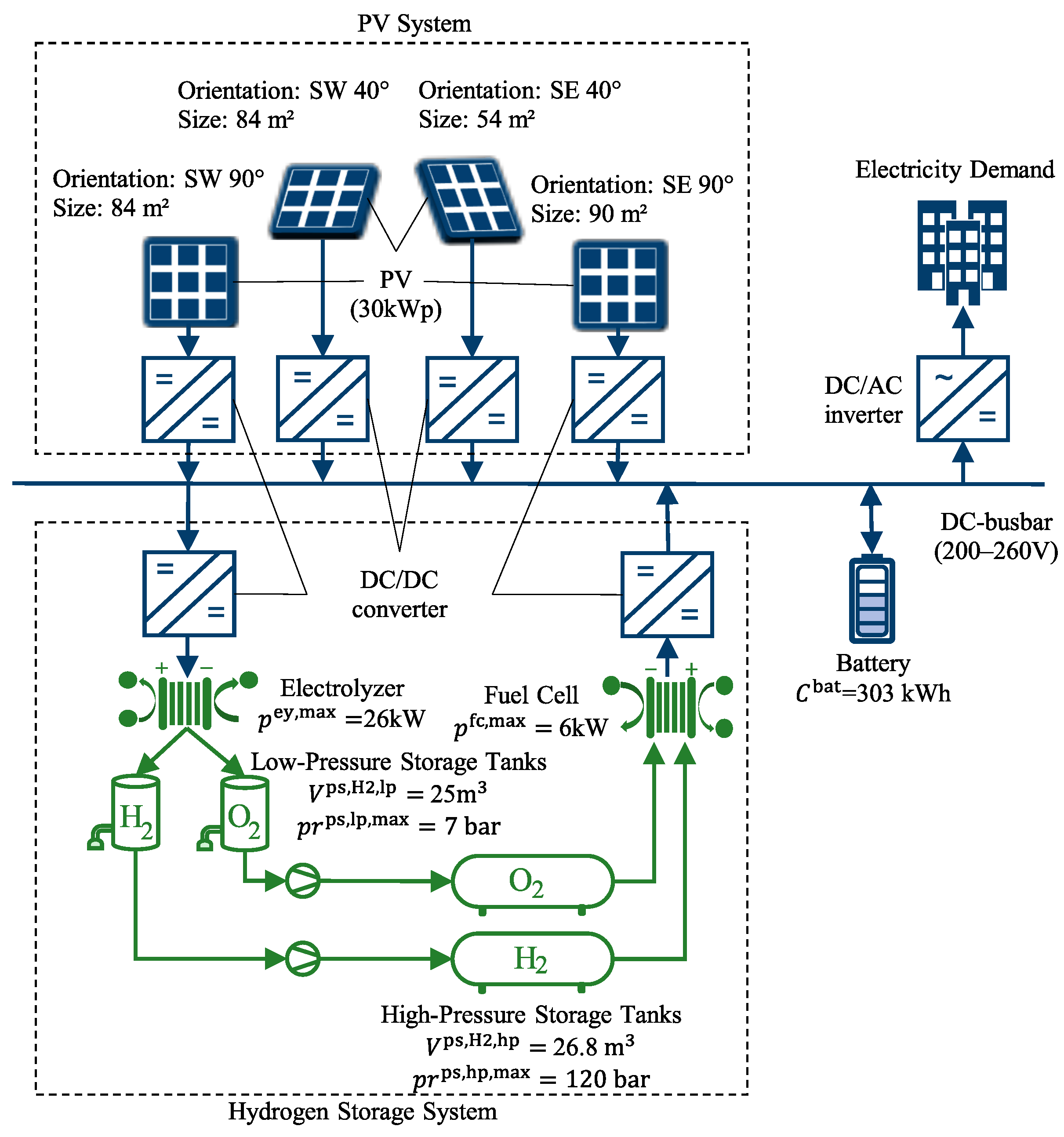
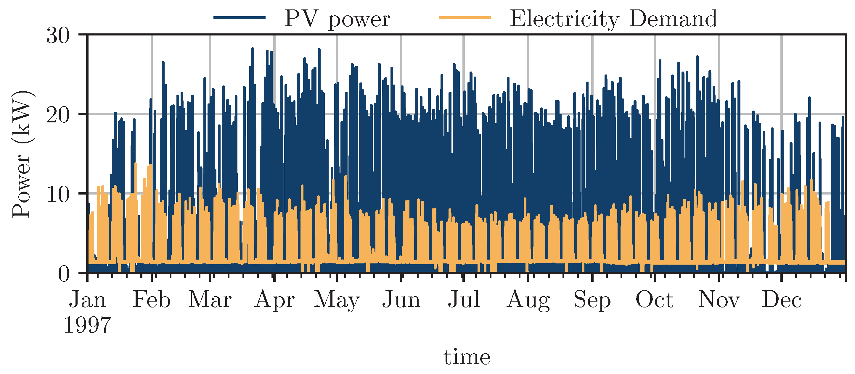
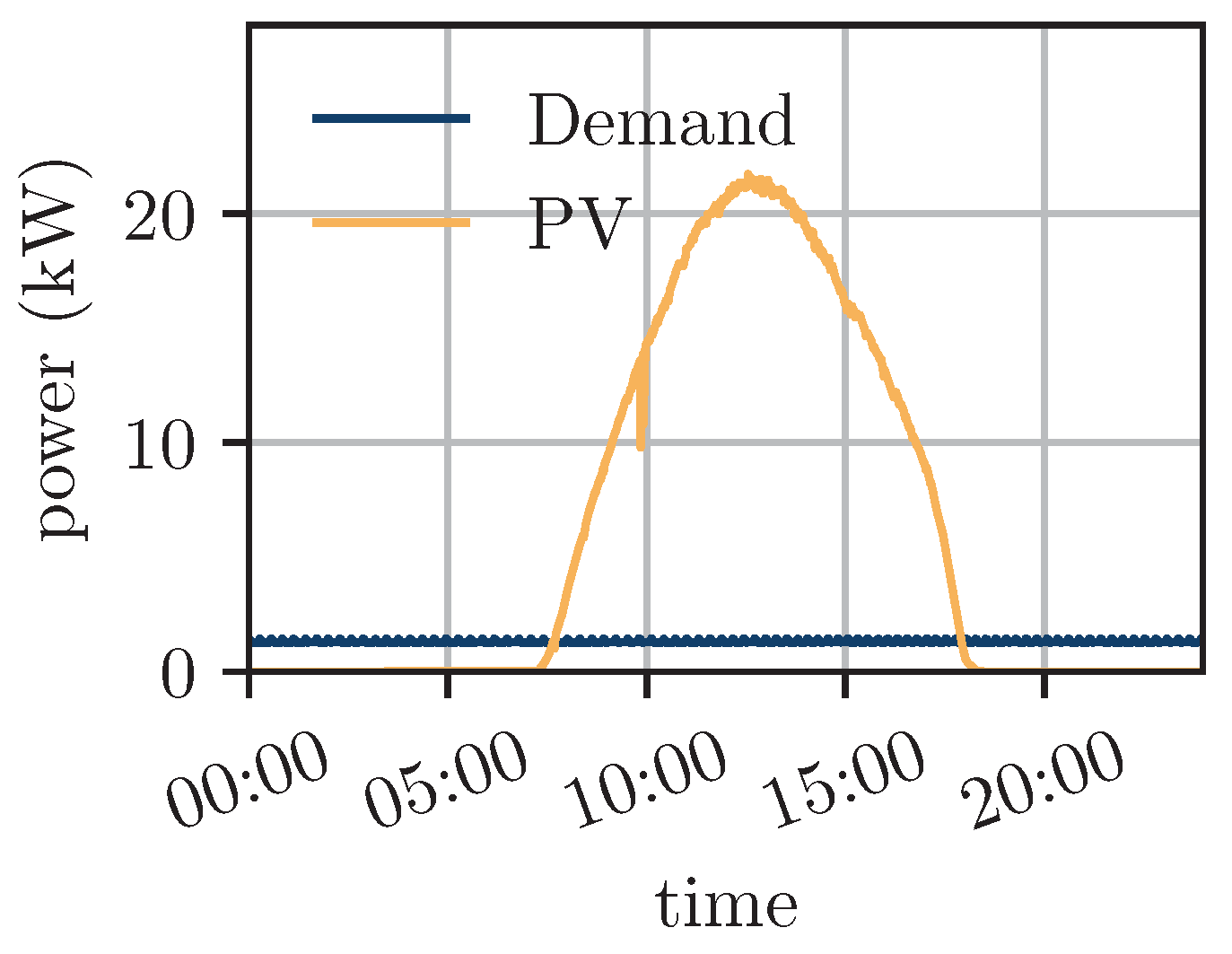
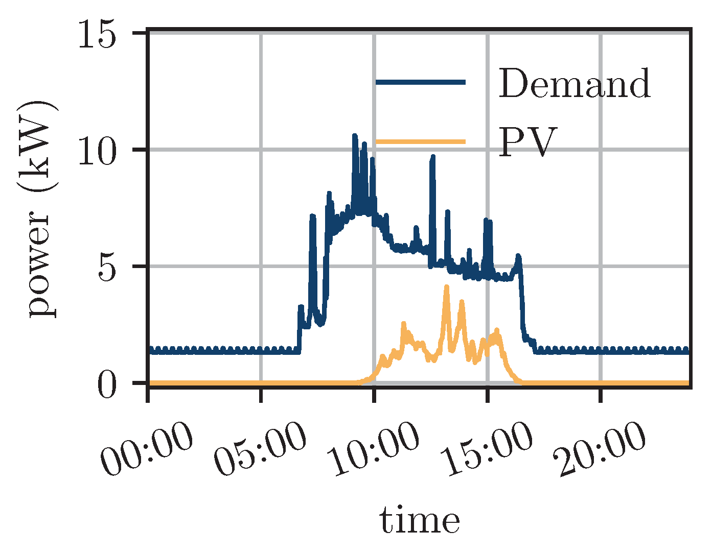
2.1. Simulation Model
2.2. Detailed Optimization Model
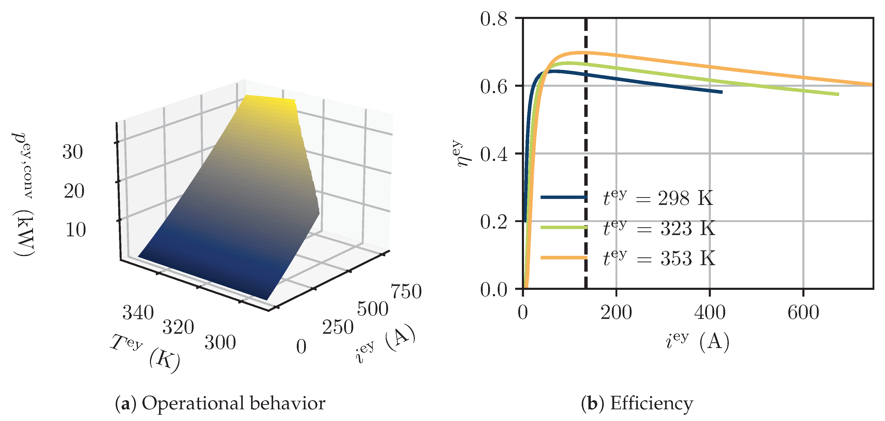
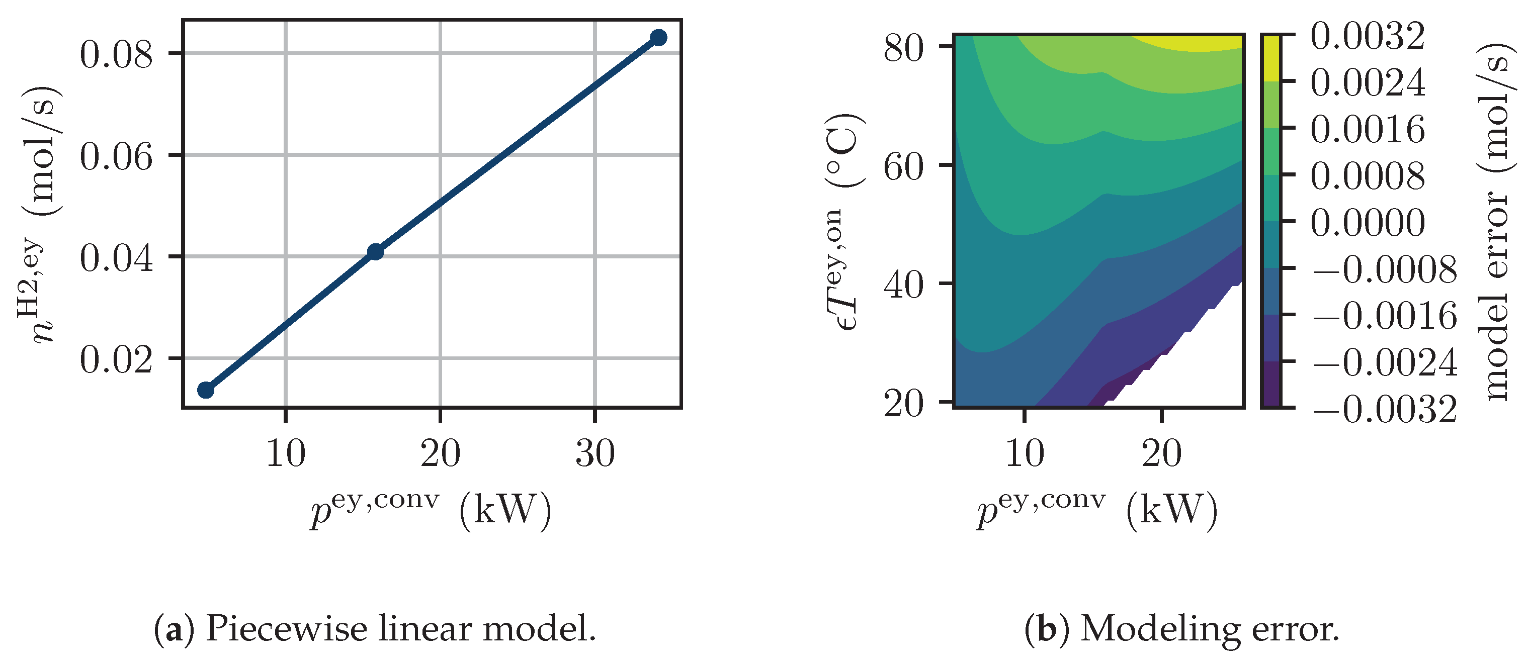
2.2.1. Electrolyzer
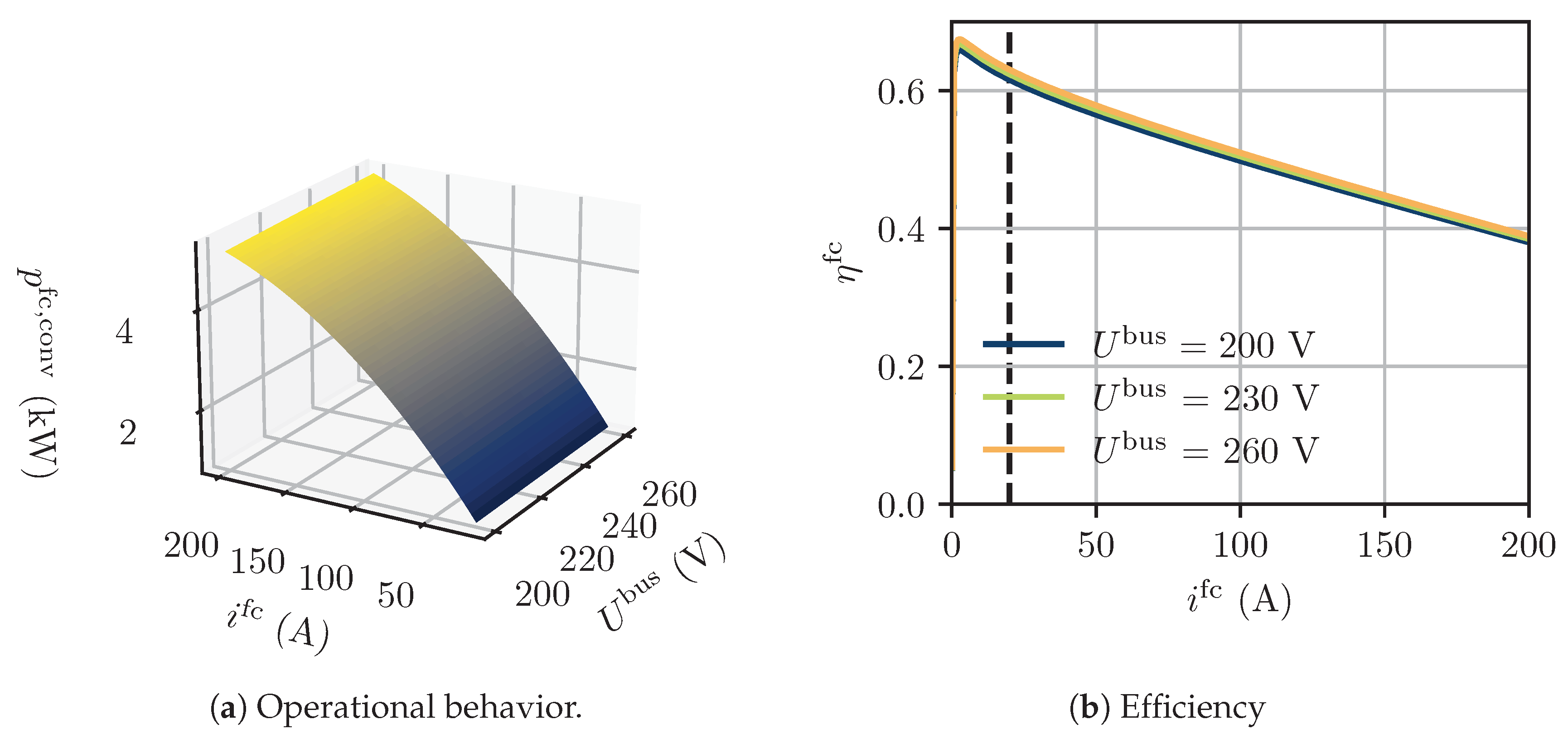
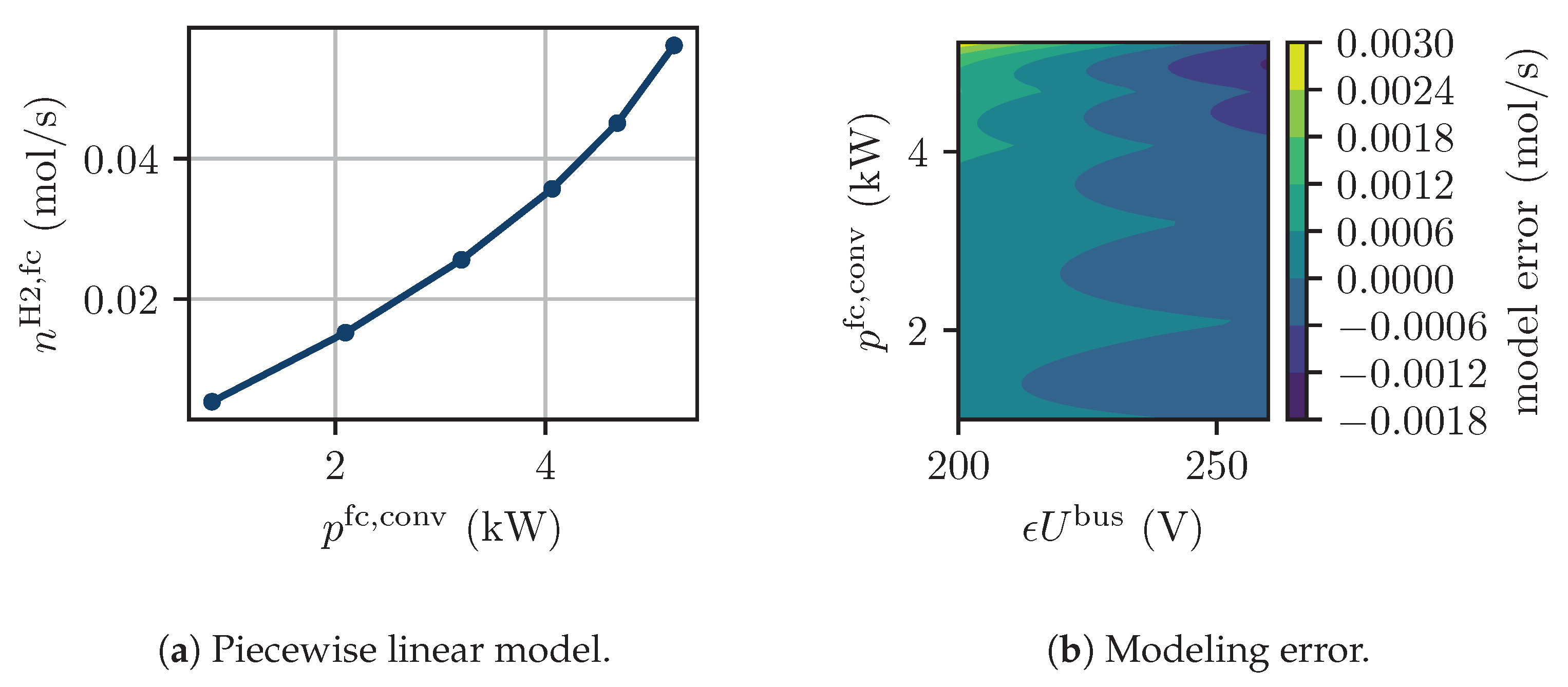
2.2.2. Fuel Cell
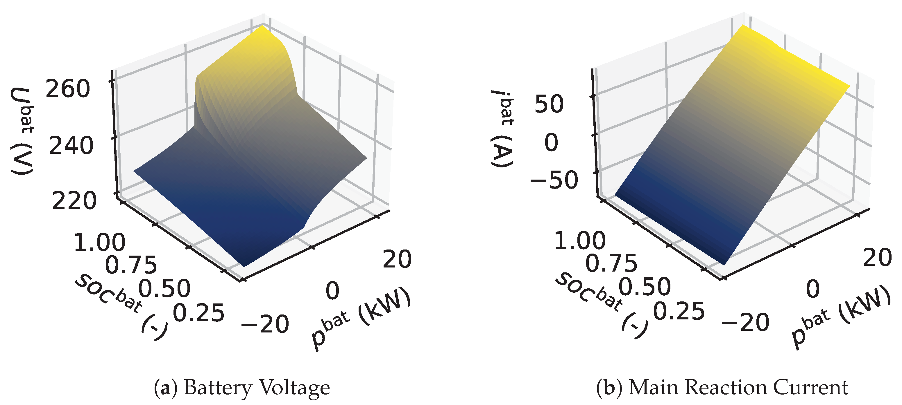
2.2.3. Battery
2.2.4. Pressure Storage
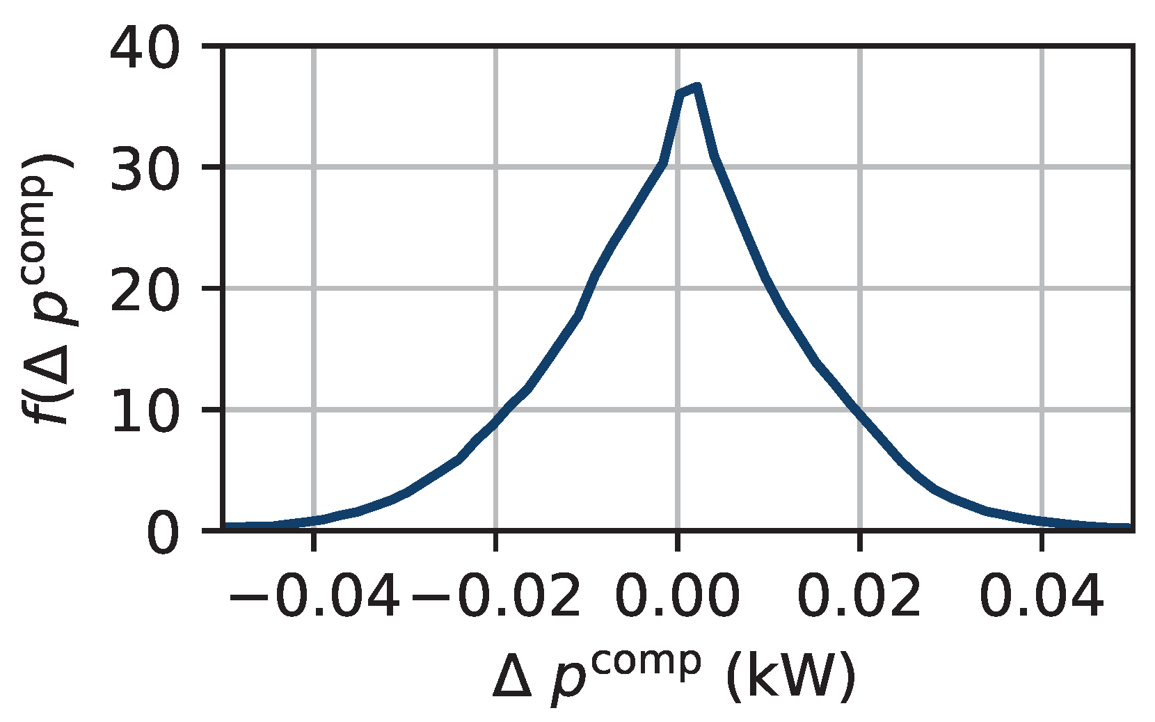
2.2.5. Compressor
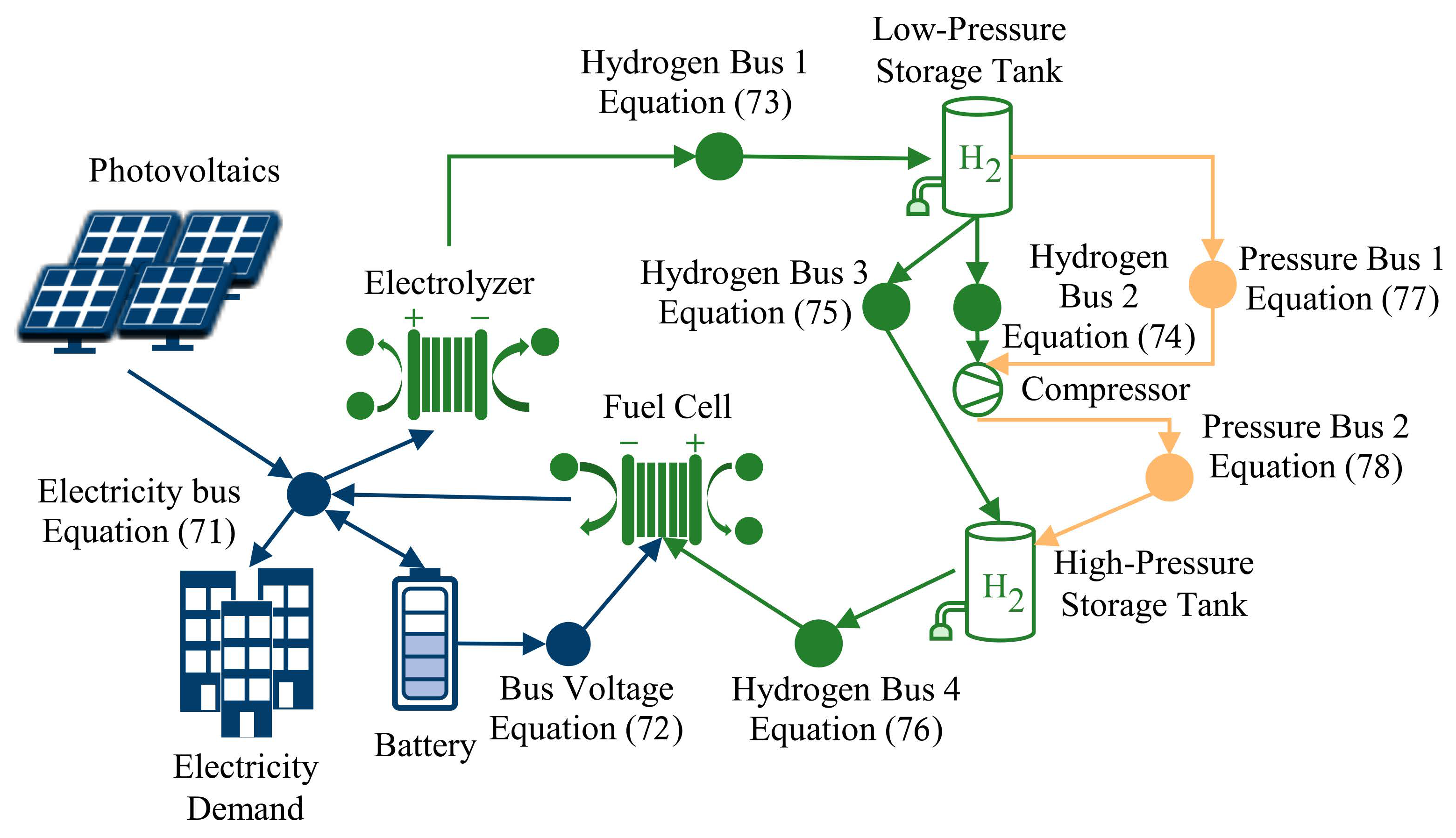
2.2.6. Energy System
2.3. Simplified Optimization Model
3. Case Study
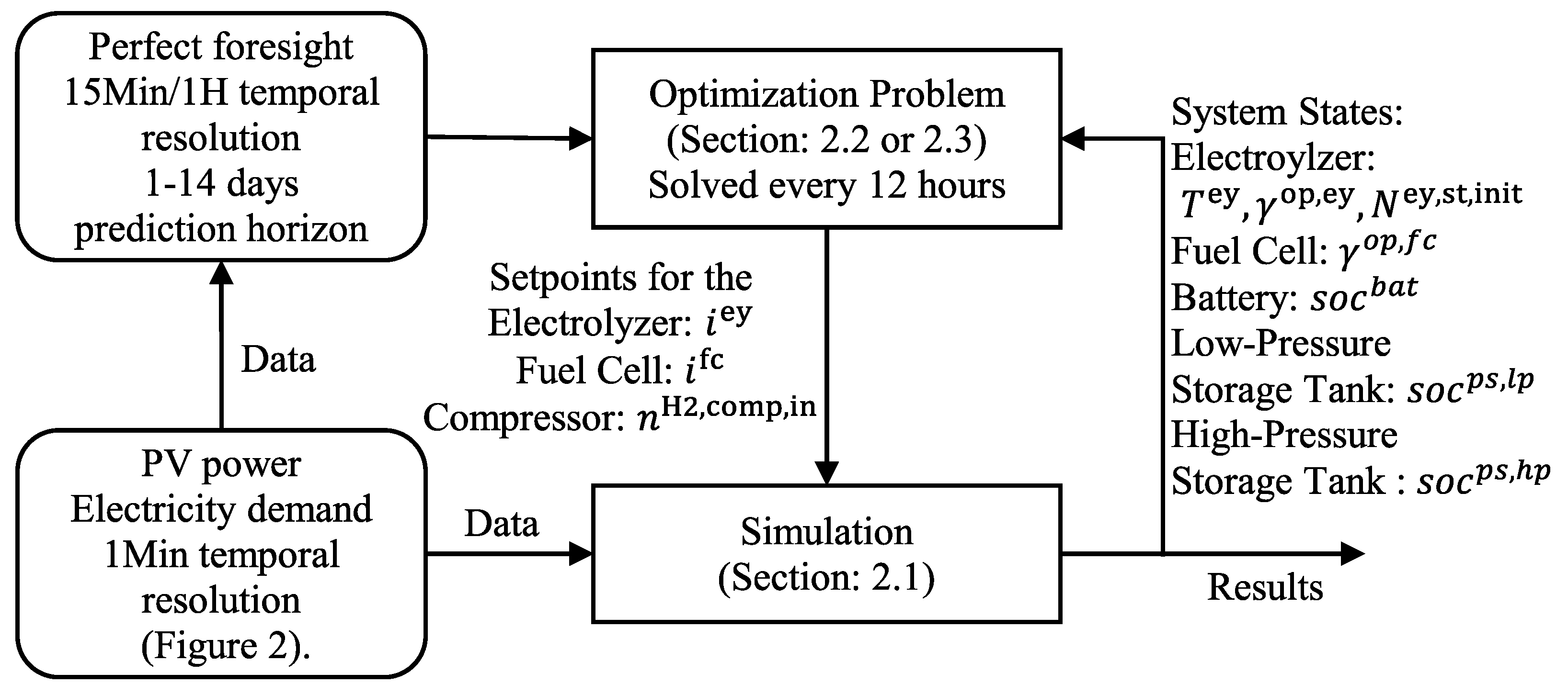
3.1. Model Predictive Control Framework
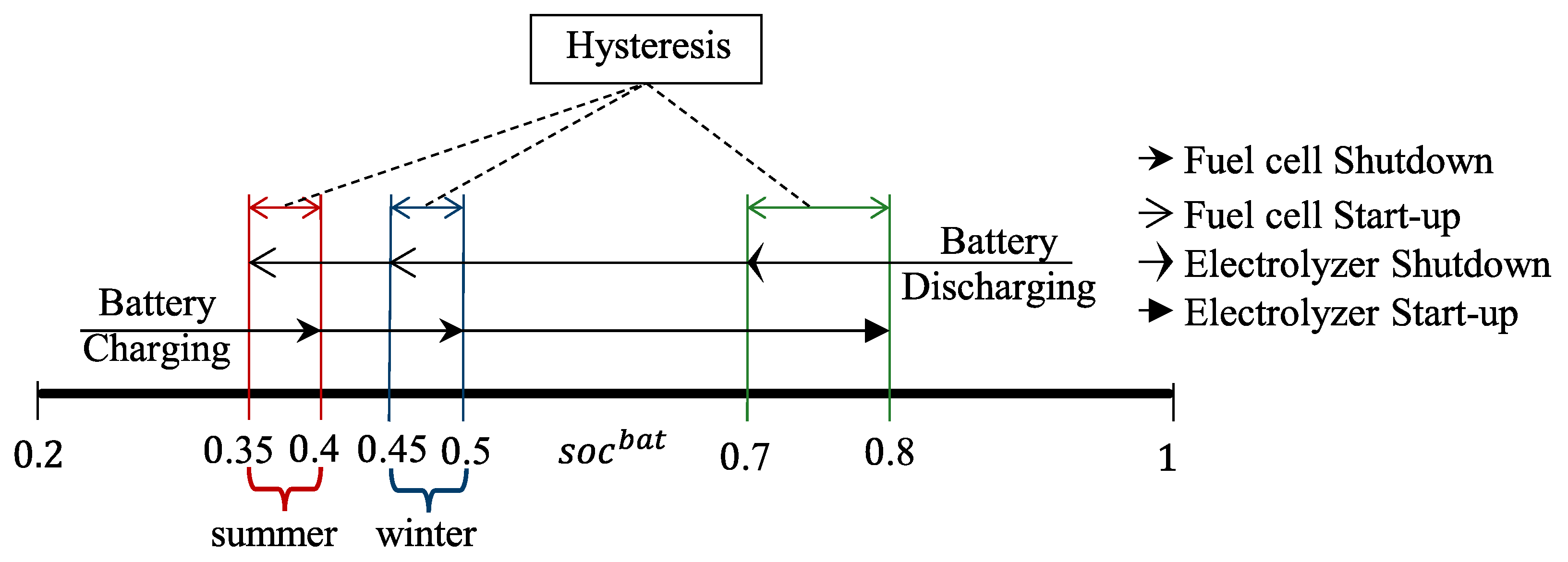
3.2. Hysteresis Band Controller
4. Results
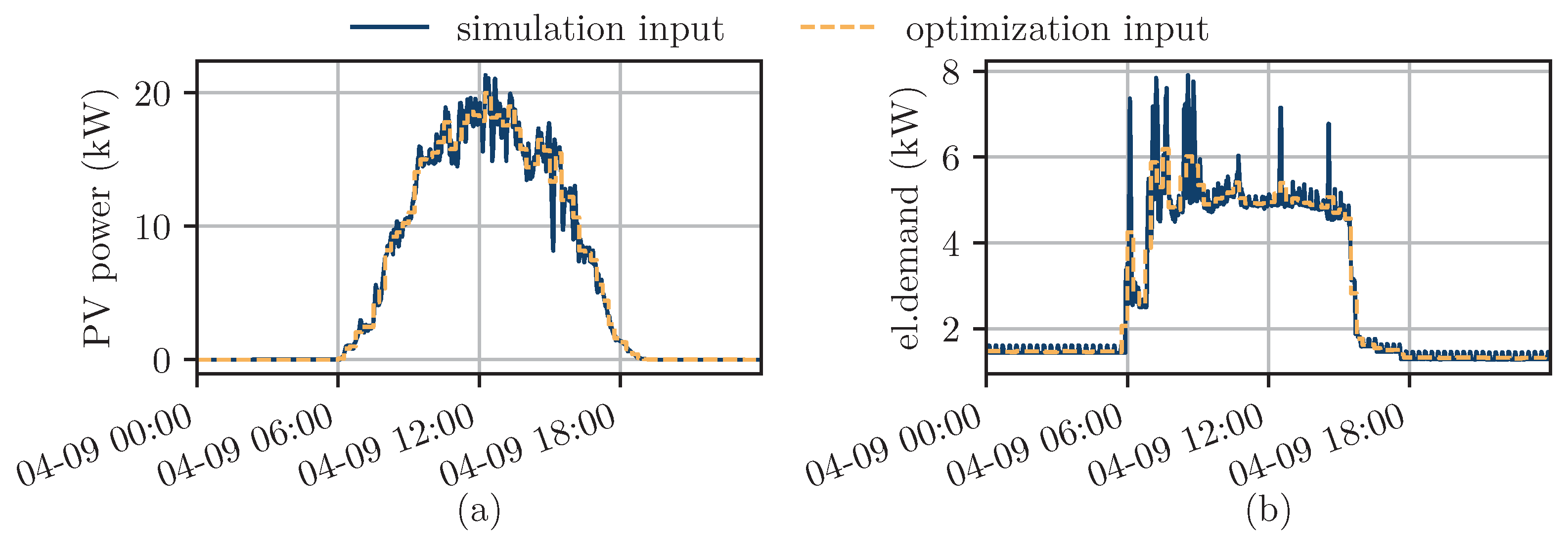
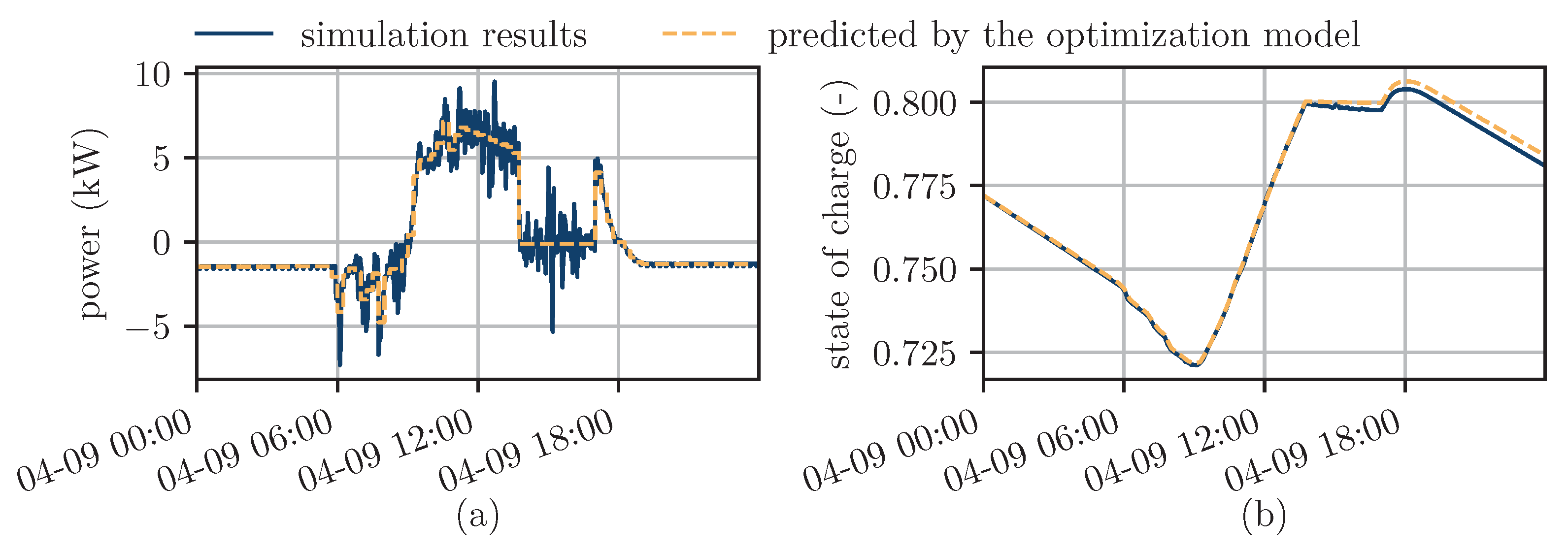
4.1. Comparison between Optimization and Simulation Results
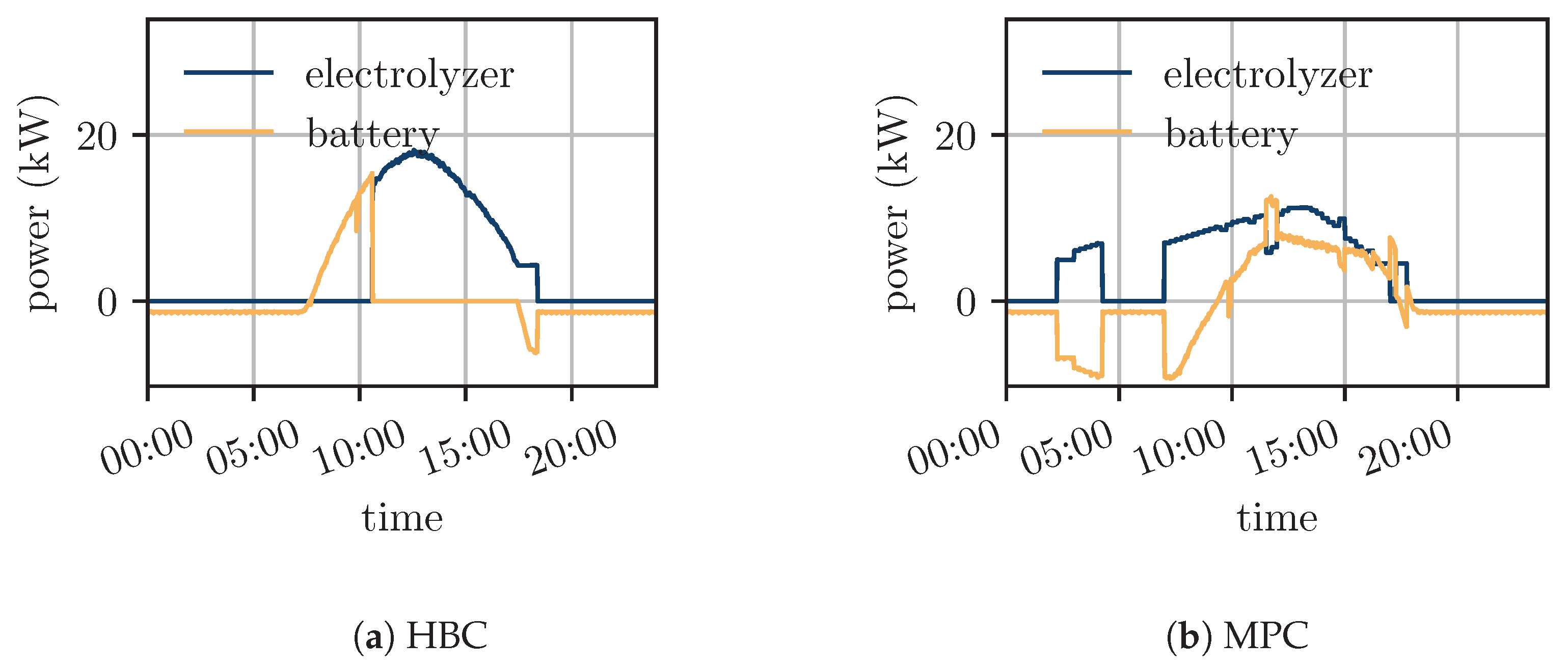
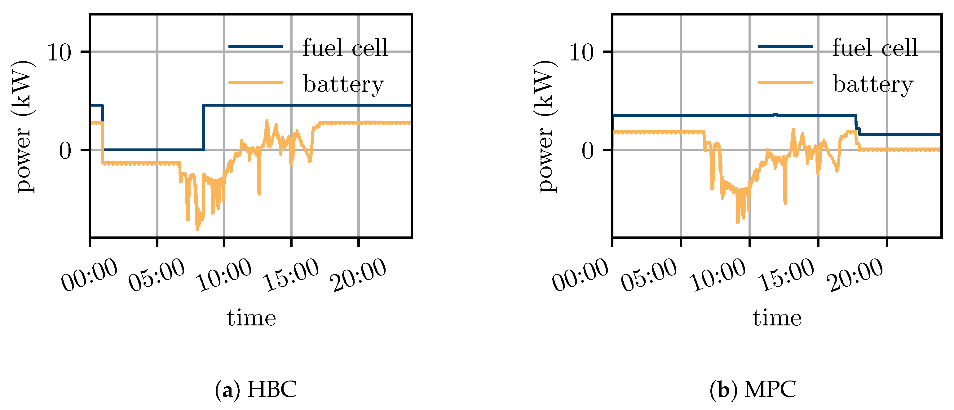
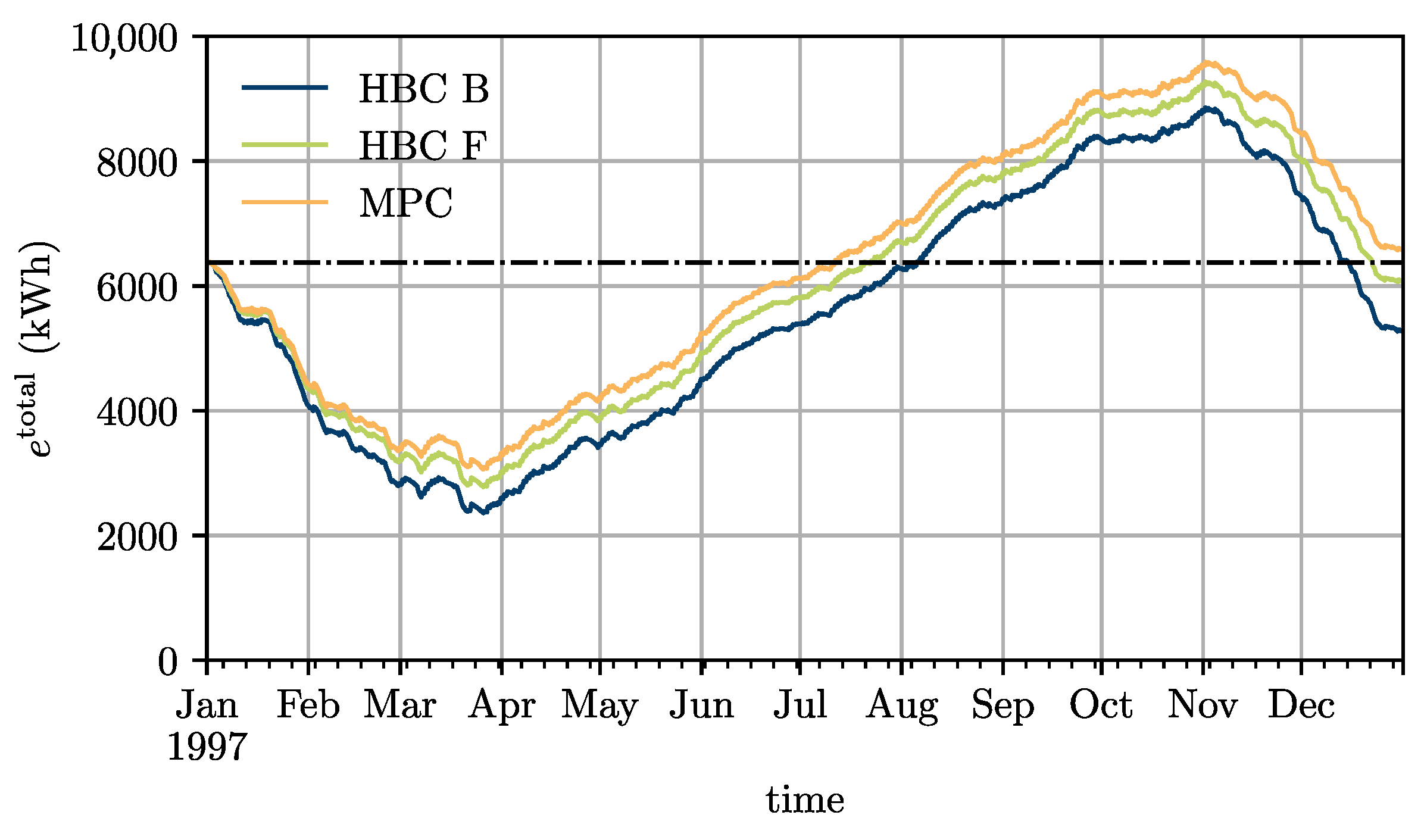
4.2. Comparison between the Model Predictive Controller and the Hysteresis Band Controller
4.3. Comparison between MPC Runs
5. Conclusions
Author Contributions
Funding
Data Availability Statement
Acknowledgments
Conflicts of Interest
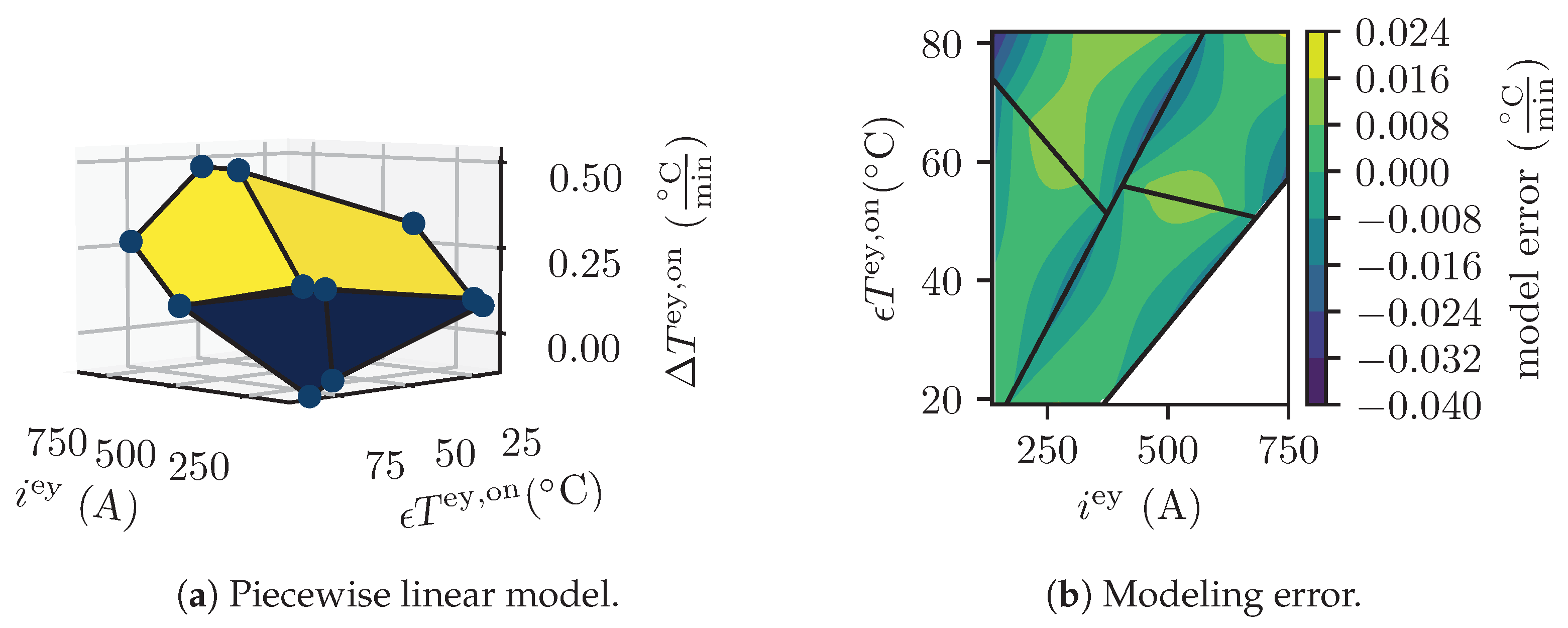
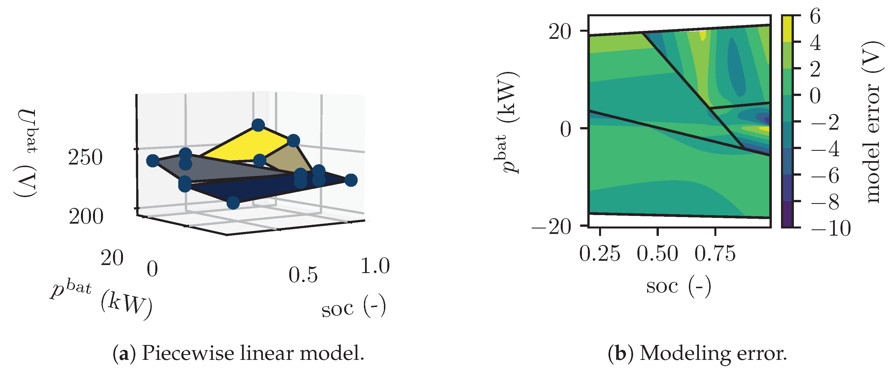
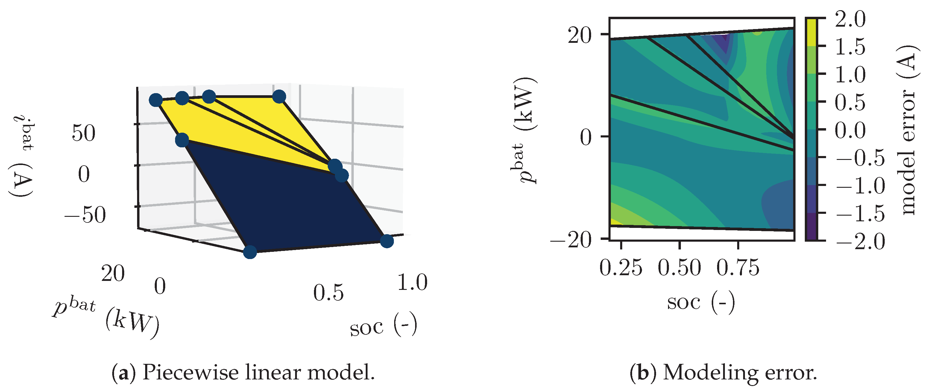
Appendix A. Piecewise Linear Models
Appendix A.1. Electrolyzer Power

| Constant | Value | Constant | Value | Constant | Value |
|---|---|---|---|---|---|
| 135.0 | −1.00 | −750. | |||
| −82.0 | 19.0 | 0.0990 | |||
| −17.3 | −0.995 | 401.4 | |||
| 82.0 | 750.0 | 59.9 | |||
| 628.0 | 0.00679 | −0.628 | |||
| −0.0256 | 1.18 | −0.000112 | |||
| −0.0187 | 0.979 | 0.0236 | |||
| −0.00463 | 0.000112 | 0.0187 | |||
| −1.18 | 0.00463 | −0.979 | |||
| −0.0236 | 0.628 | 0.0256 | |||
| −0.00679 | 0.298 | 0.0418 | |||
| 0.0464 | 0.0506 | 0.0505 | |||
| −0.0131 | −0.0735 | −1.21 | |||
| −0.0331 | −0.0155 | −0.0485 | |||
| −0.0674 |
Appendix A.2. Electrolyzer Temperature Change
| Constant | Value | Constant | Value | Constant | Value |
|---|---|---|---|---|---|
| 135.0 | −1.00 | −750. | |||
| −82.0 | 19.0 | 0.0990 | |||
| −17.3 | −0.995 | 683.1 | |||
| 55.9 | 750.0 | 82.0 | |||
| 574.6 | 373.8 | 74.1 | |||
| 0.000812 | 0.0424 | −2.70 | |||
| 0.339 | 0.0547 | −0.00839 | |||
| 2.70 | −0.000812 | −0.0424 | |||
| 1.88 | −0.00208 | −0.0216 | |||
| 0.00839 | −0.339 | −0.0547 | |||
| 0.00208 | 0.0216 | −1.88 | |||
| 0.0158 | 0.447 | 0.00919 | |||
| 2.72 | 3.24 | 0.809 | |||
| 0.00721 | 0.0149 | −0.0437 | |||
| −0.0842 | −0.127 | −0.0660 |
Appendix A.3. Fuel Cell Power
| Constant | Value | Constant | Value | Constant | Value |
|---|---|---|---|---|---|
| 200.0 | −1.00 | 20.0 | |||
| −200 | −260. | 260.0 | |||
| 153.3 | 95.0 | 1.14 | |||
| 0.000373 | −0.00808 | 0.00808 | |||
| −1.14 | −0.000373 | 1.08 | |||
| 0.00108 | −0.0143 | 0.0143 | |||
| −1.08 | −0.00108 | 0.0945 | |||
| 0.857 | 1.98 | 0.0325 | |||
| 0.00153 | 0.0219 | 0.000725 | |||
| 0.0139 | 0.00192 |
Appendix A.4. Battery Voltage
| Constant | Value | Constant | Value | Constant | Value |
|---|---|---|---|---|---|
| −0.659 | −11.4 | −0.752 | |||
| 1.18 | −0.990 | 0.200 | |||
| −1.00 | 0.341 | −6.29 | |||
| −0.940 | 0.990 | 5.22 | |||
| −5.58 | 0.990 | 21.2 | |||
| 0.879 | 19.7 | −4.29 | |||
| 0.990 | 3.59 | −18.4 | |||
| 2.19 | −2.01 | −9.50 | |||
| 24.8 | −31.0 | −0.577 | |||
| 5.32 | −0.900 | −10.4 | |||
| 2.01 | 9.50 | −2.19 | |||
| 31.0 | 0.577 | −24.8 | |||
| 0.900 | 10.4 | −5.32 | |||
| 0.866 | 0.667 | 198.6 | |||
| 52.0 | 13.7 | 0.316 | |||
| 2.85 | 200.7 | 42.5 | |||
| 220.8 | 221.7 | 14.0 |
Appendix A.5. Battery Current
| Constant | Value | Constant | Value | Constant | Value |
|---|---|---|---|---|---|
| −0.659 | −11.4 | −0.752 | |||
| 1.18 | −0.990 | 0.200 | |||
| −1.00 | 0.341 | −6.29 | |||
| −0.940 | 0.990 | 21.2 | |||
| −0.111 | 19.9 | −0.483 | |||
| 0.990 | 19.5 | −2.73 | |||
| 0.990 | 8.16 | −18.4 | |||
| 10.3 | −0.241 | −10.5 | |||
| 0.241 | 10.5 | −10.3 | |||
| 10.9 | −11.2 | −0.354 | |||
| 11.2 | 0.354 | −10.9 | |||
| 5.66 | −0.519 | −7.15 | |||
| 0.519 | 7.15 | −5.66 | |||
| 1.12 | 15.8 | 5.37 | |||
| 1.73 | 3.75 | 4.12 | |||
| 4.45 | 3.99 | −0.597 | |||
| −16.4 | −2.10 | −5.90 |
Appendix A.6. Compressor
| Constant | Value | Constant | Value | Constant | Value |
|---|---|---|---|---|---|
| 0.0124 | −1.00 | 8.00 | |||
| −7.00 | −0.0619 | −120. | |||
| 2.00 | 5.56 | 120.0 | |||
| 0.0619 | 7.00 | 120.0 | |||
| 0.0619 | 7.00 | 89.6 | |||
| 6.55 | 89.3 | 0.0619 | |||
| 5.40 | 42.3 | 0.0317 | |||
| 0.0704 | −0.00117 | −4.58 | |||
| 0.00325 | 6.06 | −0.0360 | |||
| −0.00404 | 0.00117 | 4.58 | |||
| −0.0317 | −0.0704 | 0.00104 | |||
| 3.78 | −0.00841 | −0.0487 | |||
| 0.0360 | 0.00404 | −0.00325 | |||
| −6.06 | 4.09 | −0.00857 | |||
| −0.0101 | −0.00532 | 0.00841 | |||
| 0.0487 | −0.00104 | −3.78 | |||
| 0.00857 | 0.0101 | 0.00532 | |||
| −4.09 | 0.00108 | 0.000534 | |||
| 0.0147 | 0.00258 | 5.14 | |||
| 0.00145 | 9.25 | 0.00469 | |||
| 0.0103 | 0.00523 | 3.45 | |||
| 9.28 | 13.8 | -0.00710 | |||
| −0.0305 | −0.0898 | −0.0235 | |||
| −0.0621 | −0.0727 | −0.0218 |
Appendix A.7. Electrolyzer Power Simplified
| Constant | Value | Constant | Value | Constant | Value |
|---|---|---|---|---|---|
| 15.6 | 4.85 | 34.1 | |||
| 0.00446 | 0.00166 | 0.00230 | |||
| 0.00248 |
Appendix A.8. Fuel Cell Power Simplified
| Constant | Value | Constant | Value | Constant | Value |
|---|---|---|---|---|---|
| 2.21 | 0.827 | 3.32 | |||
| 4.14 | 4.71 | 5.23 | |||
| 0.00964 | 0.0121 | 0.0206 | |||
| 0.00784 | 0.0155 | −0.0273 | |||
| −0.00515 | −0.0132 | −0.00117 | |||
| −0.0516 |
References
- Umweltbundesamt. Erneuerbare Energien in Deutschland 2020: Daten zur Entwicklung im Jahr 2020; Umweltbundesamt: Dessau-Roßlau, Germany, 2021. [Google Scholar]
- Marocco, P.; Ferrero, D.; Martelli, E.; Santarelli, M.; Lanzini, A. An MILP approach for the optimal design of renewable battery-hydrogen energy systems for off-grid insular communities. Energy Convers. Manag. 2021, 245, 114564. [Google Scholar] [CrossRef]
- Le, T.S.; Nguyen, T.N.; Bui, D.K.; Ngo, T.D. Optimal sizing of renewable energy storage: A techno-economic analysis of hydrogen, battery and hybrid systems considering degradation and seasonal storage. Appl. Energy 2023, 336, 120817. [Google Scholar] [CrossRef]
- Ulleberg, Ø. Stand-Alone Power Systems for the Future: Optimal Design, Operation and Control of Solar-Hydrogen Energy Systems; Operation & Control of Solar-Hydrogen Energy Systems: Trondheim, Norway, 1998. [Google Scholar]
- Gabrielli, P.; Gazzani, M.; Martelli, E.; Mazzotti, M. Optimal design of multi-energy systems with seasonal storage. Appl. Energy 2018, 219, 408–424. [Google Scholar] [CrossRef]
- Kotzur, L.; Markewitz, P.; Robinius, M.; Stolten, D. Time series aggregation for energy system design: Modeling seasonal storage. Appl. Energy 2018, 213, 123–135. [Google Scholar] [CrossRef]
- Petkov, I.; Gabrielli, P. Power-to-hydrogen as seasonal energy storage: An uncertainty analysis for optimal design of low-carbon multi-energy systems. Appl. Energy 2020, 274, 115197. [Google Scholar] [CrossRef]
- Marocco, P.; Ferrero, D.; Lanzini, A.; Santarelli, M. The role of hydrogen in the optimal design of off-grid hybrid renewable energy systems. J. Energy Storage 2022, 46, 103893. [Google Scholar] [CrossRef]
- Chauhan, A.; Saini, R.P. A review on Integrated Renewable Energy System based power generation for stand-alone applications: Configurations, storage options, sizing methodologies and control. Renew. Sustain. Energy Rev. 2014, 38, 99–120. [Google Scholar] [CrossRef]
- Ipsakis, D.; Voutetakis, S.; Seferlis, P.; Stergiopoulos, F.; Elmasides, C. Power management strategies for a stand-alone power system using renewable energy sources and hydrogen storage. Int. J. Hydrogen Energy 2009, 34, 7081–7095. [Google Scholar] [CrossRef]
- Olatomiwa, L.; Mekhilef, S.; Ismail, M.S.; Moghavvemi, M. Energy management strategies in hybrid renewable energy systems: A review. Renew. Sustain. Energy Rev. 2016, 62, 821–835. [Google Scholar] [CrossRef]
- Modu, B.; Abdullah, M.P.; Bukar, A.L.; Hamza, M.F. A systematic review of hybrid renewable energy systems with hydrogen storage: Sizing, optimization, and energy management strategy. Int. J. Hydrogen Energy 2023, 48, 38354–38373. [Google Scholar] [CrossRef]
- Bordons, C.; Garcia-Torres, F.; Ridao, M.A. Model Predictive Control of Microgrids; Springer: Berlin/Heidelberg, Germany, 2020; Volume 358. [Google Scholar] [CrossRef]
- Modu, B.; Abdullah, M.P.; Bukar, A.L.; Hamza, M.F.; Adewolu, M.S. Energy management and capacity planning of photovoltaic-wind-biomass energy system considering hydrogen-battery storage. J. Energy Storage 2023, 73, 109294. [Google Scholar] [CrossRef]
- Li, Z.; Liu, Y.; Du, M.; Cheng, Y.; Shi, L. Modeling and multi-objective optimization of a stand-alone photovoltaic-wind turbine-hydrogen-battery hybrid energy system based on hysteresis band. Int. J. Hydrogen Energy 2023, 48, 7959–7974. [Google Scholar] [CrossRef]
- Alili, H.; Mahmoudimehr, J. Techno-economic assessment of integrating hydrogen energy storage technology with hybrid photovoltaic/pumped storage hydropower energy system. Energy Convers. Manag. 2023, 294, 117437. [Google Scholar] [CrossRef]
- Garcia-Torres, F.; Valverde, L.; Bordons, C. Optimal Load Sharing of Hydrogen-Based Microgrids With Hybrid Storage Using Model-Predictive Control. IEEE Trans. Ind. Electron. 2016, 63, 4919–4928. [Google Scholar] [CrossRef]
- Valverde, L.; Bordons, C.; Rosa, F. Integration of Fuel Cell Technologies in Renewable-Energy-Based Microgrids Optimizing Operational Costs and Durability. IEEE Trans. Ind. Electron. 2016, 63, 167–177. [Google Scholar] [CrossRef]
- Garcia-Torres, F.; Bordons, C. Optimal Economical Schedule of Hydrogen-Based Microgrids With Hybrid Storage Using Model Predictive Control. IEEE Trans. Ind. Electron. 2015, 62, 5195–5207. [Google Scholar] [CrossRef]
- Cau, G.; Cocco, D.; Petrollese, M.; Knudsen Kær, S.; Milan, C. Energy management strategy based on short-term generation scheduling for a renewable microgrid using a hydrogen storage system. Energy Convers. Manag. 2014, 87, 820–831. [Google Scholar] [CrossRef]
- Fan, F.; Zhang, R.; Xu, Y. Robustly coordinated operation of an emission-free microgrid with hybrid hydrogen-battery energy storage. CSEE J. Power Energy Syst. 2021, 8, 369–379. [Google Scholar] [CrossRef]
- Li, Q.; Qiu, Y.; Yang, H.; Xu, Y.; Chen, W.; Wang, P. Stability-constrained two-stage robust optimization for integrated hydrogen hybrid energy system. CSEE J. Power Energy Syst. 2020, 7, 162–171. [Google Scholar] [CrossRef]
- Cardona, P.; Costa-Castelló, R.; Roda, V.; Carroquino, J.; Valiño, L.; Serra, M. Model predictive control of an on-site green hydrogen production and refuelling station. Int. J. Hydrogen Energy 2023, 48, 17995–18010. [Google Scholar] [CrossRef]
- Gonzalez-Rivera, E.; Garcia-Trivino, P.; Sarrias-Mena, R.; Torreglosa, J.P.; Jurado, F.; Fernandez-Ramirez, L.M. Model Predictive Control-Based Optimized Operation of a Hybrid Charging Station for Electric Vehicles. IEEE Access 2021, 9, 115766–115776. [Google Scholar] [CrossRef]
- Yassuda Yamashita, D.; Vechiu, I.; Gaubert, J.P. Two-level hierarchical model predictive control with an optimised cost function for energy management in building microgrids. Appl. Energy 2021, 285, 116420. [Google Scholar] [CrossRef]
- Thaler, B.; Posch, S.; Wimmer, A.; Pirker, G. Hybrid model predictive control of renewable microgrids and seasonal hydrogen storage. Int. J. Hydrogen Energy 2023, 161, 48. [Google Scholar] [CrossRef]
- Neisen, V.; Baader, F.J.; Abel, D. Supervisory Model-based Control using Mixed Integer Optimization for stationary hybrid fuel cell systems. IFAC-PapersOnLine 2018, 51, 320–325. [Google Scholar] [CrossRef]
- Weimann, L.; Gabrielli, P.; Boldrini, A.; Kramer, G.J.; Gazzani, M. Optimal hydrogen production in a wind-dominated zero-emission energy system. Adv. Appl. Energy 2021, 3, 100032. [Google Scholar] [CrossRef]
- Yassuda Yamashita, D.; Vechiu, I.; Gaubert, J.P.; Jupin, S. Autonomous observer of hydrogen storage to enhance a model predictive control structure for building microgrids. J. Energy Storage 2022, 53, 105072. [Google Scholar] [CrossRef]
- Huang, C.; Zong, Y.; You, S.; Træholt, C. Economic model predictive control for multi-energy system considering hydrogen-thermal-electric dynamics and waste heat recovery of MW-level alkaline electrolyzer. Energy Convers. Manag. 2022, 265, 115697. [Google Scholar] [CrossRef]
- Abdelghany, M.B.; Al-Durra, A.; Zeineldin, H.; Hu, J. Integration of cascaded coordinated rolling horizon control for output power smoothing in islanded wind–solar microgrid with multiple hydrogen storage tanks. Energy 2024, 291, 130442. [Google Scholar] [CrossRef]
- Abdelghany, M.B.; Al-Durra, A.; Daming, Z.; Gao, F. Optimal multi-layer economical schedule for coordinated multiple mode operation of wind–solar microgrids with hybrid energy storage systems. J. Power Sources 2024, 591, 233844. [Google Scholar] [CrossRef]
- Li, Z.; Xia, Y.; Bo, Y.; Wei, W. Optimal planning for electricity-hydrogen integrated energy system considering multiple timescale operations and representative time-period selection. Appl. Energy 2024, 362, 122965. [Google Scholar] [CrossRef]
- Birkelbach, F.; Huber, D.; Hofmann, R. Piecewise linear approximation for MILP leveraging piecewise convexity to improve performance. Comput. Chem. Eng. 2024, 183, 108596. [Google Scholar] [CrossRef]
- Neisen, V.; Futing, M.; Abel, D. Optimization Approaches for Model Predictive Power Flow Control in Hybrid Fuel Cell Systems. In Proceedings of the IECON 2019—45th Annual Conference of the IEEE Industrial Electronics Society, Lisbon, Portugal, 14–17 October 2019; IEEE: Piscataway, NJ, USA, 2019; pp. 4575–4582. [Google Scholar] [CrossRef]
- Ulleberg, Ø. Modeling of advanced alkaline electrolyzers: A system simulation approach. Int. J. Hydrogen Energy 2003, 28, 21–33. [Google Scholar] [CrossRef]
- Li, B.; Miao, H.; Li, J. Multiple hydrogen-based hybrid storage systems operation for microgrids: A combined TOPSIS and model predictive control methodology. Appl. Energy 2021, 283, 116303. [Google Scholar] [CrossRef]
- Khaligh, V.; Ghezelbash, A.; Zarei, M.; Liu, J.; Won, W. Efficient integration of alkaline water electrolyzer – A model predictive control approach for a sustainable low-carbon district heating system. Energy Convers. Manag. 2023, 292, 117404. [Google Scholar] [CrossRef]
- Pan, G.; Gu, W.; Lu, Y.; Qiu, H.; Lu, S.; Yao, S. Optimal Planning for Electricity-Hydrogen Integrated Energy System Considering Power to Hydrogen and Heat and Seasonal Storage. IEEE Trans. Sustain. Energy 2020, 11, 2662–2676. [Google Scholar] [CrossRef]
- Kämper, A.; Holtwerth, A.; Leenders, L.; Bardow, A. AutoMoG 3D: Automated Data-Driven Model Generation of Multi-Energy Systems Using Hinging Hyperplanes. Front. Energy Res. 2021, 9, 719658. [Google Scholar] [CrossRef]
- Holtwerth, A.; Xhonneux, A.; Muller, D. Data-Driven Generation of Mixed-Integer Linear Programming Formulations for Model Predictive Control of Hybrid Energy Storage Systems using detailed nonlinear Simulation Models. In Proceedings of the 2022 Open Source Modelling and Simulation of Energy Systems (OSMSES), Aachen, Germany, 4–5 April 2022; IEEE: Piscataway, NJ, USA, 2022; pp. 1–6. [Google Scholar] [CrossRef]
- Holtwerth, A. LinMoG: Linear Model Generation. 2024. Available online: https://jugit.fz-juelich.de/iek-10/public/optimization/linmog (accessed on 15 January 2024).
- Wakui, T.; Akai, K.; Yokoyama, R. Shrinking and receding horizon approaches for long-term operational planning of energy storage and supply systems. Energy 2022, 239, 122066. [Google Scholar] [CrossRef]
- Guo, Z.; Wei, W.; Bai, J.; Mei, S. Long-term operation of isolated microgrids with renewables and hybrid seasonal-battery storage. Appl. Energy 2023, 349, 121628. [Google Scholar] [CrossRef]
- Abdelghany, M.B.; Shehzad, M.F.; Liuzza, D.; Mariani, V.; Glielmo, L. Optimal operations for hydrogen-based energy storage systems in wind farms via model predictive control. Int. J. Hydrogen Energy 2021, 46, 29297–29313. [Google Scholar] [CrossRef]
- Abdelghany, M.B.; Al-Durra, A.; Zeineldin, H.; Gao, F. Integrating scenario-based stochastic-model predictive control and load forecasting for energy management of grid-connected hybrid energy storage systems. Int. J. Hydrogen Energy 2023, 48, 35624–35638. [Google Scholar] [CrossRef]
- Abdelghany, M.B.; Mariani, V.; Liuzza, D.; Glielmo, L. Hierarchical model predictive control for islanded and grid-connected microgrids with wind generation and hydrogen energy storage systems. Int. J. Hydrogen Energy 2024, 51, 595–610. [Google Scholar] [CrossRef]
- Holtwerth, A.; Xhonneux, A.; Müller, D. Closed Loop Model Predictive Control of a Hybrid Battery-Hydrogen Energy Storage System using Mixed-Integer Linear Programming. Energy Convers. Manag. X 2024, 22, 100561. [Google Scholar] [CrossRef]
- Barthels, H.; Brocke, W.A.; Bonhoff, K.; Groehn, H.G.; Heuts, G.; Lennartz, M.; Mai, H.; Mergel, J.; Schmid, L.; Ritzenhoff, P. Phoebus-Jülich: An autonomous energy supply system comprising photovoltaics, electrolytic hydrogen, fuel cell. Int. J. Hydrogen Energy 1998, 23, 295–301. [Google Scholar] [CrossRef]
- Barthels, H. PHOEBUS—Das Jülicher System Photovoltaik-Elektrolyse-Brennstoffzelle; Springer: Berlin/Heidelberg, Germany, 1996. [Google Scholar]
- Meurer, C.; Barthels, H.; Brocke, W.A.; Emonts, B.; Groehn, H.G. PHOEBUS—An autonomous supply system with renewable energy: Six years of operational experience and advanced concepts. Sol. Energy 1999, 67, 131–138. [Google Scholar] [CrossRef]
- Ghosh, P.; Emonts, B.; Janßen, H.; Mergel, J.; Stolten, D. Ten years of operational experience with a hydrogen-based renewable energy supply system. Sol. Energy 2003, 75, 469–478. [Google Scholar] [CrossRef]
- Langiu, M.; Shu, D.Y.; Baader, F.J.; Hering, D.; Bau, U.; Xhonneux, A.; Müller, D.; Bardow, A.; Mitsos, A.; Dahmen, M. COMANDO: A Next-Generation Open-Source Framework for Energy Systems Optimization. Comput. Chem. Eng. 2021, 152, 107366. [Google Scholar] [CrossRef]
- Gurobi Optimization LLC. Gurobi Optimizer Reference Manual; Gurobi Optimization LLC: Beaverton, OR, USA, 2022. [Google Scholar]


| Component Name | Parameter | Value |
|---|---|---|
| Electrolyzer | 750 A | |
| 135 A | ||
| 40 V | ||
| 26 kW | ||
| 80 °C | ||
| 7 bar | ||
| Fuel Cell | 200 A | |
| 20 A | ||
| 6 kW | ||
| Battery | 200–260 V | |
| 80 A | ||
| 303 kWh | ||
| Pressure Storage | 25 m3 | |
| 7 bar | ||
| 26.8 m3 | ||
| 120 bar | ||
| PV | 30 kW | |
| 27.18 MWh | ||
| Demand | 13.73 kW | |
| 19.76 MWh |
| Hysteresis Band Controller | |||
|---|---|---|---|
| Name | Description | ||
| HBC B | HBC with fixed fuel cell hydrogen input of around 3 | ||
| HBC F | HBC with a flexible fuel cell and maximal power output of 5.20 kW | ||
| Model Predictive Controller | |||
| Name | Optimization Model | Prediction Horizon | Temporal Resolution |
| MPC D 1D 15M | Detailed | 1 Day | 15 min |
| MPC S 1D 15M | Simplified | 1 Day | 15 min |
| MPC S 4D 15M | Simplified | 4 Day | 15 min |
| MPC S 4D 1H | Simplified | 4 Day | 1 h |
| MPC S 7D 1H | Simplified | 7 Day | 1 h |
| MPC S 7D 1H | Simplified | 14 Day | 1 h |
| MPC D 1D 15M | HBC B | HBC F | |
|---|---|---|---|
| Controller | MPC | HBC | HBC |
| Fuel Cell Operation | Flexible | Fixed Volume Flow | Flexible |
| Prediction Horizon | 1 Day | - | - |
| Temporal Resolution | 15 min | - | - |
| (kWh) | 6570.65 | 5264.86 | 6061.73 |
| 0.724 | 0.721 | 0.721 | |
| (kWh) | 9081.08 | 9276.62 | 9290.35 |
| 0.591 | 0.512 | 0.563 | |
| (kWh) | 3708.91 | 3960.40 | 3905.51 |
| 326 | 161 | 160 | |
| (kW) | 8439.16 | 33,948.79 | 34,042.73 |
| 24 | 93 | 27 | |
| (kW) | 537.61 | 854.57 | 4780.54 |
| MPC D 1D 15M | MPC S 1D 15M | MPC S 4D 15M | MPC S 4D 1H | MPC S 7D 1H | MPC S 14D 1H | |
|---|---|---|---|---|---|---|
| Optimization Model | Detailed | Simplified | Simplified | Simplified | Simplified | Simplified |
| Prediction Horizon | 1 Day | 1 Day | 4 Days | 4 Days | 7 Days | 14 Days |
| Temporal Resolution | 15 min | 15 min | 15 min | 1 h | 1 h | 1 h |
| (kWh) | 6570.65 | 6096.62 | 7037.81 | 6907.51 | 7070.36 | 7205.98 |
| 0.724 | 0.728 | 0.727 | 0.725 | 0.727 | 0.731 | |
| (kWh) | 9081.08 | 9278.95 | 9052.45 | 8965.67 | 8973.24 | 8924.64 |
| 0.591 | 0.593 | 0.616 | 0.617 | 0.624 | 0.63 | |
| (kWh) | 3708.91 | 4103.06 | 3585.76 | 3616.26 | 3571.90 | 3520.4 |
| 326 | 236 | 155 | 176 | 153 | 153 | |
| (kW) | 8439.16 | 3601.19 | 3675.68 | 3665.34 | 2955.72 | 1963.08 |
| 24 | 31 | 26 | 23 | 23 | 24 | |
| (kW) | 537.61 | 608.48 | 361.72 | 281.37 | 267.50 | 237.1 |
| avg. run time (s) | 44.81 | 26.53 | 70.02 | 27.05 | 38.30 | 66.54 |
| max. run time (s) | 548.67 | 50.08 | 189.32 | 82.82 | 79.86 | 192.75 |
Disclaimer/Publisher’s Note: The statements, opinions and data contained in all publications are solely those of the individual author(s) and contributor(s) and not of MDPI and/or the editor(s). MDPI and/or the editor(s) disclaim responsibility for any injury to people or property resulting from any ideas, methods, instructions or products referred to in the content. |
© 2024 by the authors. Licensee MDPI, Basel, Switzerland. This article is an open access article distributed under the terms and conditions of the Creative Commons Attribution (CC BY) license (https://creativecommons.org/licenses/by/4.0/).
Share and Cite
Holtwerth, A.; Xhonneux, A.; Müller, D. Model Predictive Control of a Stand-Alone Hybrid Battery-Hydrogen Energy System: A Case Study of the PHOEBUS Energy System. Energies 2024, 17, 4720. https://doi.org/10.3390/en17184720
Holtwerth A, Xhonneux A, Müller D. Model Predictive Control of a Stand-Alone Hybrid Battery-Hydrogen Energy System: A Case Study of the PHOEBUS Energy System. Energies. 2024; 17(18):4720. https://doi.org/10.3390/en17184720
Chicago/Turabian StyleHoltwerth, Alexander, André Xhonneux, and Dirk Müller. 2024. "Model Predictive Control of a Stand-Alone Hybrid Battery-Hydrogen Energy System: A Case Study of the PHOEBUS Energy System" Energies 17, no. 18: 4720. https://doi.org/10.3390/en17184720
APA StyleHoltwerth, A., Xhonneux, A., & Müller, D. (2024). Model Predictive Control of a Stand-Alone Hybrid Battery-Hydrogen Energy System: A Case Study of the PHOEBUS Energy System. Energies, 17(18), 4720. https://doi.org/10.3390/en17184720