Abstract
Domestic hot water (DHW) consumption represents a significant portion of household energy usage, prompting the exploration of smart heat pump technology to efficiently meet DHW demands while minimizing energy waste. This paper proposes an innovative investigation of models using deep learning and continual learning algorithms to personalize DHW predictions of household occupants’ behavior. Such models, alongside a control system that decides when to heat, enable the development of a heat-pumped-based smart DHW production system, which can heat water only when needed and avoid energy loss due to the storage of hot water. Deep learning models, and attention-based models particularly, can be used to predict time series efficiently. However, they suffer from catastrophic forgetting, meaning that when they dynamically learn new patterns, older ones tend to be quickly forgotten. In this work, the continuous learning of DHW consumption prediction has been addressed by benchmarking proven continual learning methods on both real dwelling and synthetic DHW consumption data. Task-per-task analysis reveals, among the data from real dwellings that do not present explicit distribution changes, a gain compared to the non-evolutive model. Our experiment with synthetic data confirms that continual learning methods improve prediction performance.
1. Introduction
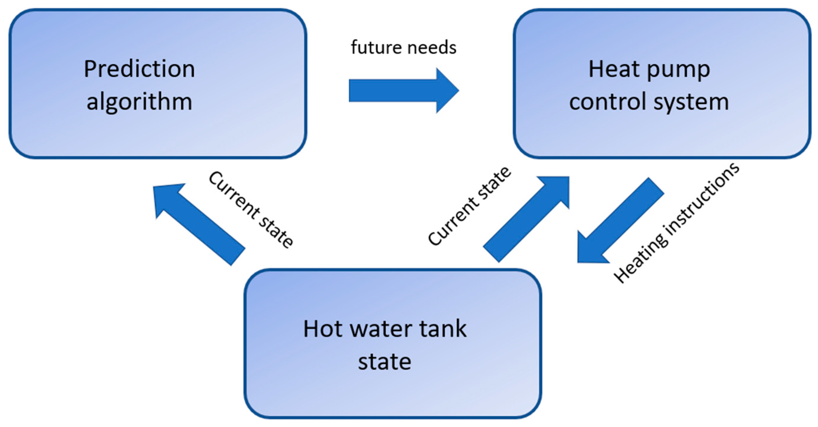
Prediction of domestic hot water (DHW) consumption is an important task for energy savings in residential buildings, as it enables avoiding losing energy by storing hot water, which necessarily becomes colder due to the imperfect insulation of the hot water tank. DHW prediction helps heat water only when the inhabitants of the house need it. Such anticipation is particularly critical when the heating system cannot produce large quantities of hot water quickly enough, as is the case with individual housing heat pumps. Note that the prediction model has to be linked to a control system that decides when to heat water depending on both the DHW consumption predictions and the thermodynamics of the heating system. This present work focuses only on the prediction model. A schematic view of the interaction between the prediction and the control system is presented in Figure 1.

Figure 1.
Schematic view of a smart domestic hot water management system.
In the field of machine learning and, more specifically, deep learning, several models can be used for time series forecasting. Among the machine learning models, XGBoost is a model that has been used for various time series prediction issues but requires prior feature extraction [1,2], while ARIMA is a model that has been widely used for time series prediction [3,4]. Among deep learning, the recurrent neural network (RNN) and its variations, such as long-short term memory (LSTM), gated recurrent unit (GRU) [5,6,7], and the convolutional neural network (CNN) [8,9], are models that have been explored for time series prediction. In deep learning, although transformers have been initially developed for natural language processing and then extended to vision [10,11], they have demonstrated, more recently, great performance at predicting time series [12,13]. Additionally, the attention-based model has demonstrated better prediction performance than ARIMA, GRU, LSTM, and 1DCNN on a prediction task on a DHW consumption dataset [14]. Given this current state-of-the-art in time series prediction, we have chosen to implement a model relying on transformers for DHW prediction.
Another desired feature of the prediction model is its ability to continuously adapt to user habits. But, as the habits of users evolve through time, systems must have the ability to continually learn new patterns without forgetting old ones. However, it is well known that artificial neural networks are subject to catastrophic forgetting, meaning that learning new data implies the forgetting of previously learned knowledge [15]. The issue of catastrophic forgetting has been addressed by many works, giving rise to the field of continual learning, also called incremental learning. Many strategies have been developed to tackle catastrophic forgetting, often with different scenarios, most of which are associated with strong hypotheses: some continual learning algorithms require, for instance, the task’s identity at test time [16]. In the present work, we are focused on task-agnostic continual learning, meaning that the data arrive in a continuous stream and that the times when the data distributions shift are not known [17]: the model is continuously updated using the data from the last seen DHW consumption. In practice, each task corresponds to the DHW consumption for a given time interval, typically one month. This scenario, which does not assume anything on the data stream, is the hardest but is chosen here, as it describes a realistic case where DHW consumption may shift at any time depending on the inhabitants’ behaviors, which are unpredictable. Therefore, what we seek is to update the model after each task without forgetting the knowledge obtained from past tasks, which are no longer available.
There are three families of continual learning algorithms as follows [18]:
- The first family is the parameter isolation method. Parameter isolation methods rely on freezing neurons associated with previous tasks and adding new neurons to each new task [19].
- The second is regularization-based methods. This method focuses on minimizing the change in the weight that carries more information. For example, Elastic Weight Consolidation [20] uses the Fisher information to determine weights that carry more information.
- The third family is replay methods, where some previously seen examples or pseudo-examples, i.e., examples belonging to the same distribution as previously seen examples, are learned along with new examples in order to preserve the knowledge from previous tasks. Replay methods have shown the most promising results [18,21].
Therefore, the present study focuses on algorithms from this last family, the replay-based method. To the best of our knowledge, continuous learning for predicting DHW has not been addressed by any paper and no standard individual DHW time series are publicly available. Consequently, we focused on proven continual learning algorithms to provide basic results about this issue. More specifically, the present work focuses on rehearsal and pseudo-rehearsal continual learning algorithms, with a focus on the ethical issue of data privacy preservation. Three algorithms, Dream Net [22], Experience Replay [23] and Dark Experience Replay [24], which rely on rehearsal or pseudo-rehearsal mechanisms, have been implemented for predicting DHW consumption. ER and DER are relatively simple models that are known to have good performance [25,26]. We chose to implement Dream Net because, unlike DER and ER, it does not require the storage of real examples thus allowing for data privacy; this method has also shown robust performance in many different scenarios [27]. These methods also have the advantage of being task agnostic, i.e., no prior information about each task is required and no task-specific information is needed at test time.
2. Materials and Methods
2.1. Related Works
The Dream Net [22] algorithm consists of keeping track of previous knowledge by adding a reconstruction mechanism to the prediction model at training time. It uses two networks instead of one, Learning Net and Memory Net: when a new task is learned, the Learning Net is updated both with real examples from the current task and with pseudo examples generated by the Memory Net; at the end of each task, the weights of the Learning Net are copied to the Memory Net. The generation of pseudo examples with the Memory Net is carried out by performing reinjections: starting from initial noise, this noise is injected as an input to the generating model, this “reconstruction” is, in turn, reinjected into the model to be reconstructed; the pseudo examples are formed by the set of those input/output pairs obtained from the Memory Net. The hyperparameters for Dream Net are the number of reinjections for the pseudo examples generation, the number of real examples per learning batch, the number of pseudo examples per learning batch and the number of epochs for learning a task.
Experience Replay [23] is a continual learning algorithm in which examples from previous tasks are stored in a finite-size buffer and then intercalated between examples of the currently learned task. This method is based on a reservoir strategy [28], meaning that each past example has the same probability of being stored in the buffer. The hyperparameters for this method are the size of the buffer, the number of examples from the buffer in a learning batch, the number of examples from the current task in a learning batch, and the number of epochs per task.
Dark Experience Replay [24] is a continual learning algorithm that extends Experience Replay; whereas the stored examples are a pair of an input sequence and its associated ground truth targets in Experience Replay, the Dark Experience Replay algorithm adds knowledge distillation and additionally stores the result of the model prediction. In addition to the hyperparameters of Experience Replay, Dark Experience Replay uses two additional hyperparameters, α and β, which account for the strength of the learning using either the ground truth value for prediction or the passed prediction from the model as the target in the learning.
2.2. Prediction Model Description
In terms of prediction models, we decided to focus on attention-based models because they have proven to be efficient for time series prediction. Although an extensive comparison of all previously evoked machine learning and deep learning algorithms would only ensure that this model beats all other models on DHW consumption data, such a comparison is beyond the scope of this work; the focus here is to compare different continual learning algorithms given a reasonably suitable prediction model. In other words, the goal of the current work is mainly focused on continual learning and personalization rather than extensive comparisons with any machine learning and deep learning predictions on time series prediction model.
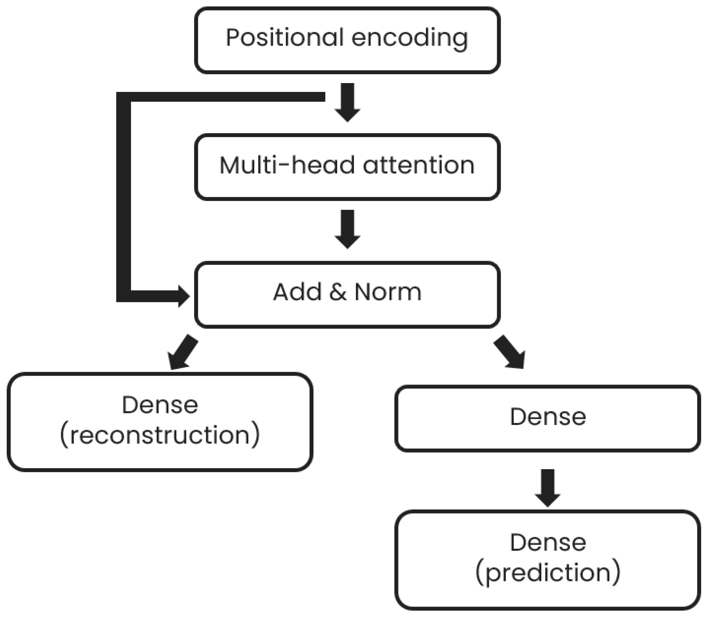
The implemented prediction model consists of a transformer block, based on the multi-head attention originally described by Vaswani et al. [10] connected to two separate dense layers, the first dense layer being used for the reconstruction of the input and the second one being used as an input for another dense layer, which provides the prediction of the time series at different time horizons, namely 0.5 h, 1 h, 2 h, 6 h, 12 h, 18 h, 24 h. Such multiple time horizon prediction is implemented to allow the control system to update its commands according to the latest prediction. A schematic description of the model is given in Figure 2. The positional encoding layer is implemented as in Vaswani’s original paper [10]. The inputs to the model are the past six days of DHW consumption, with a sampling rate of two readings per hour. The loss used for training for the prediction model is the mean square error (MSE) between the network outputs (both the reconstruction and prediction parts) and their associated ground truth.

Figure 2.
Prediction model architecture.
Multi-head attention hyperparameters and layer size are discussed in the Section 3.
2.3. Datasets Description
We study the prediction of DHW consumption with two unidimensional DHW consumption profiles measured in two different individual dwellings, referred to as Dwelling A and Dwelling B. In addition, we designed two synthetic DHW consumption profiles, from a tool we developed to generate physically plausible DHW consumption profiles with controlled randomness. The synthetic DHW consumption profiles aim to reproduce a plausible scenario in which catastrophic forgetting may occur, and thus where a continual learning algorithm would be needed; in this scenario, we consider two successively learned tasks and we evaluate the forgetting on the first task after the second one has been learned.
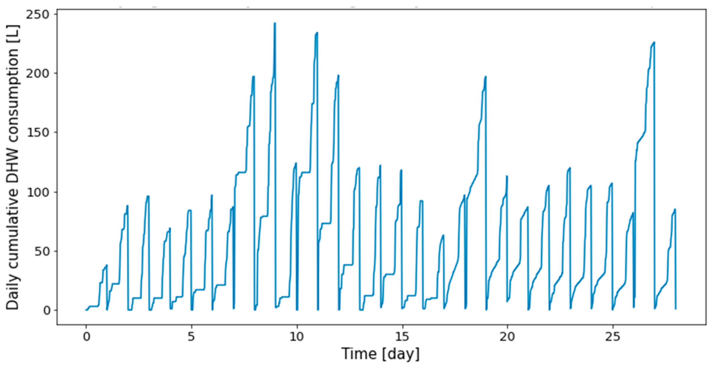
The profiles obtained from the real dwelling DHW consumptions are cumulated day by day, as can be seen in Figure 3 and Figure 4, where the consumptions of the first twenty-eight days are given, respectively, for Dwelling A and Dwelling B. The total length of the time series of Dwelling A and Dwelling B are 645 days and 737 days, with forty-eight measurements per day.
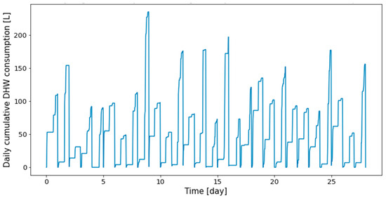
Figure 3.
First twenty-eight days of Dwelling A daily cumulative DHW consumption.
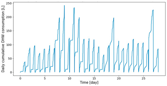
Figure 4.
First twenty-eight days of Dwelling B daily cumulative DHW consumption.
We generate synthetic DHW consumption profiles so that the DHW consumption of the j-th day, , of the week is a sum of sigmoid functions, with randomness on consumption according to the formula
with the parameters given in Table 1.

Table 1.
Parameters used for the j-th day of the week DHW consumption profile.
In addition to the data collected from real dwellings, synthetic DHW consumption profiles have been created to allow controlled DHW consumption patterns and controlled randomness. Such DHW consumption profiles are created by aggregating the days obtained with the formula for in Equation (1). We designed this formula, as a sum of sigmoid functions, so that it mimics the DHW consumption patterns in a day of real dwelling cumulative profiles, each sigmoid being associated with a particular shift and amplitude that accounts for a consumption.
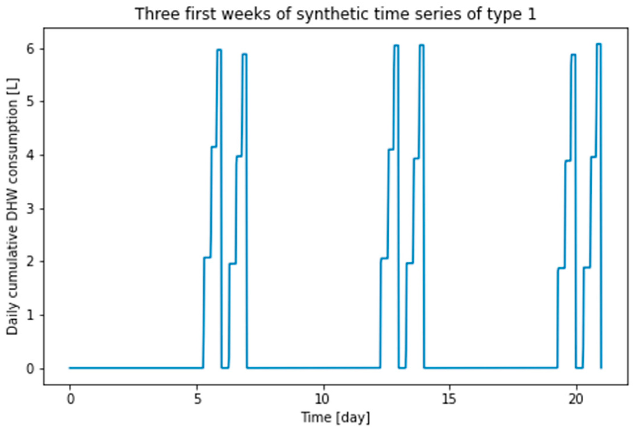
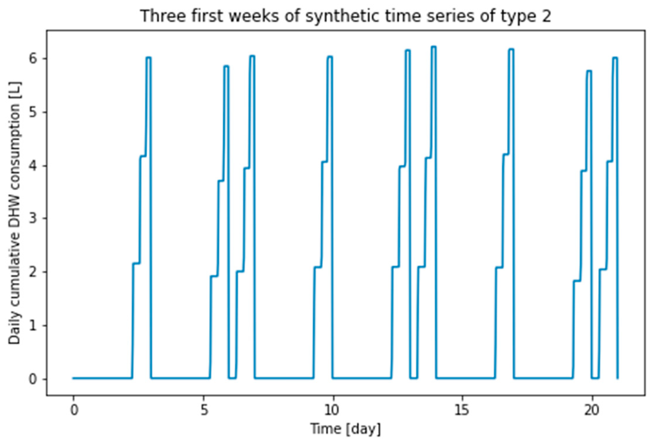
In order to create situations that make it possible to induce and test catastrophic forgetting, we present two synthetic DHW consumption profiles associated with two types of weeks corresponding to different parameterizations of Equation (1), referred to as type 1 and type 2. The parameters used for these two consumption profiles are summarized in Table 2. Qualitatively, a week of type 1 is a week in which the consumption takes place only on the weekend and a week of type 2 is a week in which the consumption takes place both on Wednesday and on the weekend. This drastic difference is (1) physically plausible and (2) subject to produce catastrophic forgetting.
Table 2.
Parameters used for constructing synthetic time series of type 1 and 2.
The first three weeks of type 1 and type 2 synthetic time series are shown in Figure 5 and Figure 6, respectively. The length of each time series is 68 weeks. These series are divided into a training part, a validation part and a testing part, with the proportions of 54%, 23% and 23%. Training data, validation data, and test data with weeks of type 1 are named d1_train, d1_valid and d1_test, respectively; training data, validation data and testing data with weeks of type 2 are named d2_train, d2_valid and d2_test, respectively.
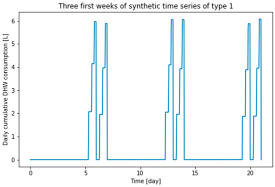
Figure 5.
First three weeks of type 1 synthetic time series.
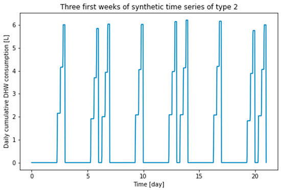
Figure 6.
First three weeks of type 2 synthetic time series.
2.4. Experiment Description—Real Dwelling Data
From the time series of the DHW consumption in real dwellings, we have implemented a realistic scenario in which we assume that the data are provided continuously, as it would be the case in a real environment, and that the model is updated at the end of each month, without access to the data of the previous months.
Specifically, in the first step, we divided the time series of the real dwelling into equal parts, called tasks, of about a month. Then, in the second step, we iteratively updated the model from each task, one after the other, without accessing other tasks.
The time series of Dwelling A and Dwelling B are divided into 21 and 26 tasks of equal length, respectively.
The continual learning algorithms we implemented are Dream Net, Dark Experience Replay and Experience Replay. These algorithms are compared to several baselines:
- -
- Finetuning, in which the model is updated on each task without any special strategies to retain knowledge from previous tasks,
- -
- One-month learning, in which the model is trained on the first task and never updated thereafter,
- -
- Three-month learning, in which the model is trained on the first three tasks and never updated thereafter,
- -
- Offline, in which the model is trained from scratch using both the current task data and all previous task data. This baseline is the upper bound for any continual learning strategy because it uses all previously seen data.
2.5. Experiment Description—Synthetic Data
We performed a first experiment with synthetic data to show, in an extreme case, the potential gain that continual learning could bring in the case of abrupt changes in resident behavior. This first experiment can be described as follows:
- -
- We first train a prediction model using d1_train;
- -
- We test this model against both d1_test and d2_test;
- -
- We train the model with different learning strategies, Dream Net, Dark Experience Replay, Finetuning on d2_train. Note that this situation should lead to catastrophic forgetting on d1_test without a continual learning algorithm;
- -
- We test the models associated with the different strategies against d1_test and d2_test to determine both whether the old data with weeks of type 1 can be accurately predicted by the models and whether the new data, with weeks of type 2, can also be accurately predicted by the model.
3. Results
3.1. Prediction Model Hyperparameters Setting
The prediction model and continual learning models need to be calibrated. To do this, we first perform a grid search on the prediction model hyperparameters. The Dwelling A time series is used as input data for this grid search.
The prediction model hyperparameters are determined by dividing the Dwelling A time series into a training set and a validation set with 80% and 20% of the data, respectively. The criterion for selecting the best hyperparameters is to minimize the mean absolute error (MAE) between the prediction and the ground truth on the validation dataset. The prediction model is trained using early stopping with a maximum number of epochs of 100 and a patience of 5.
The hyperparameters of the prediction model are the key dimension in the multi-head attention layer, the number of heads and the ratio between the number of neurons in the layer preceding the prediction layer and the layer yielding the prediction, hereafter referred to as penultimate_ratio. The hyperparameter values tested in the grid search for the prediction model and the optimal configuration obtained from this grid search are given in Table 3.
Table 3.
Hyperparameters tested in the grid search and optimal for the prediction model on the Dwelling A dataset.
3.2. Results with Real DHW Consumption of Individual Dwellings
The performance of continual learning algorithms is evaluated by measuring the mean MAE, across all the tasks, between the prediction and the ground truth, on the task following the current task. For example, considering a time series that is divided into at least three tasks, each task representing one month of data, we train the model using a given continual learning algorithm on the first month. Then, we test the trained model on the data of the second month (which the model has not yet been trained on). Then, we train the model using the same continual learning algorithm on the data of the second month’s data only. Then, we test it on the third month’s data, and so on.
The hyperparameter values tested in the grid search and the optimal configuration for the Dream Net and Dark Experience Replay algorithms are summarized in Table 4 and Table 5, respectively. The data used for this grid search are only those associated with Dwelling A. As we can see in the grid search results for DER/ER, the optimal value for α is 0, which means that in this case no distillation takes place, and it is ER and not DER that is implemented. To compare the ER and DER algorithms, we parametrize the DER algorithm from the DER/ER grid search hyperparameters, with α = 0 replaced by α = 0.5. All hyperparameters for ER and DER are summarized in the third and fourth columns of Table 5, respectively.
Table 4.
Hyperparameters tested in the grid search and optimal hyperparameters for the Dream Net algorithm on the Dwelling A dataset.
Table 5.
Hyperparameters tested in the grid search and optimal hyperparameters for the DER/ER algorithms on the Dwelling A dataset.
In the remainder of this section, we present the result of the continual learning strategies on the DHW consumption from real individual dwellings.
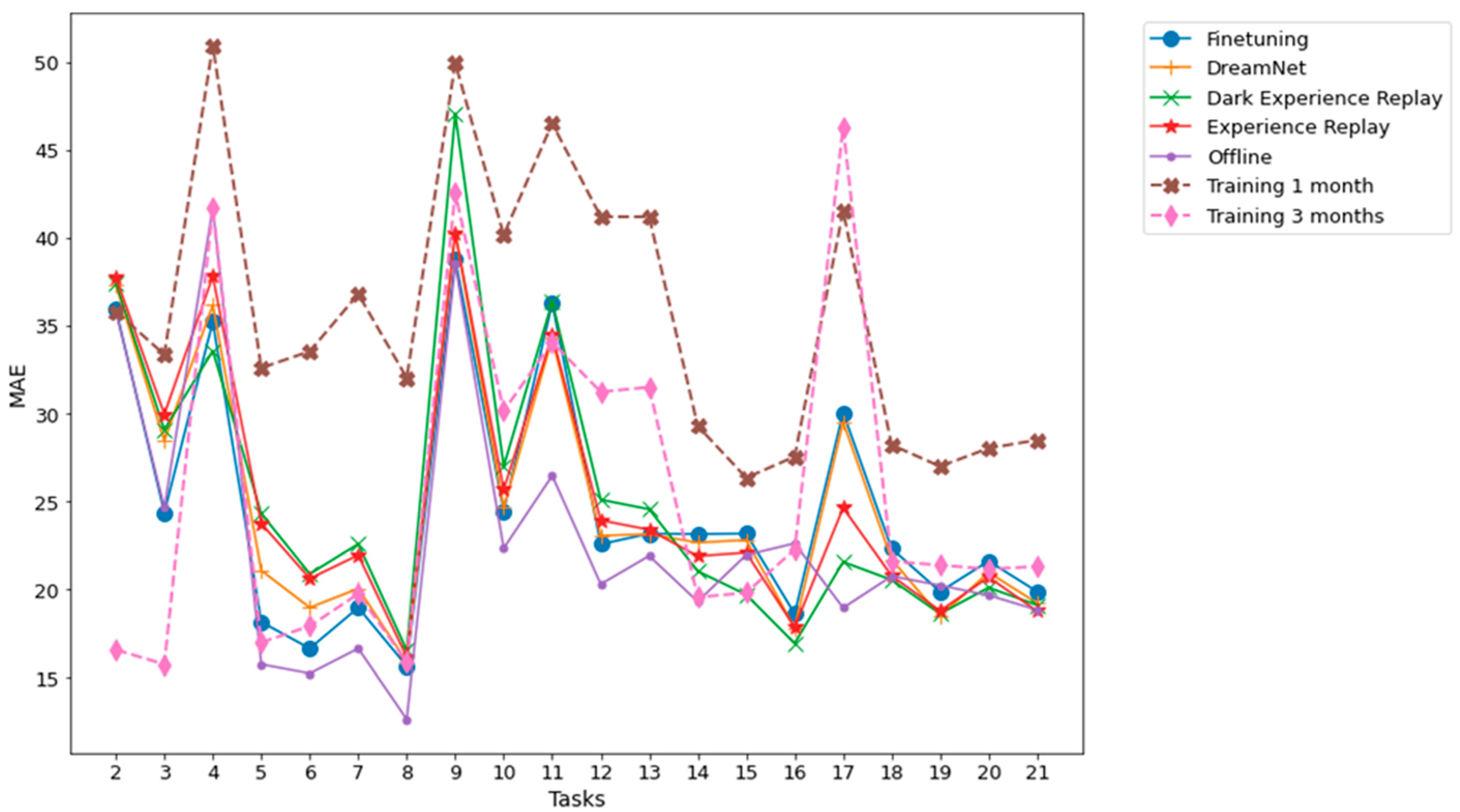
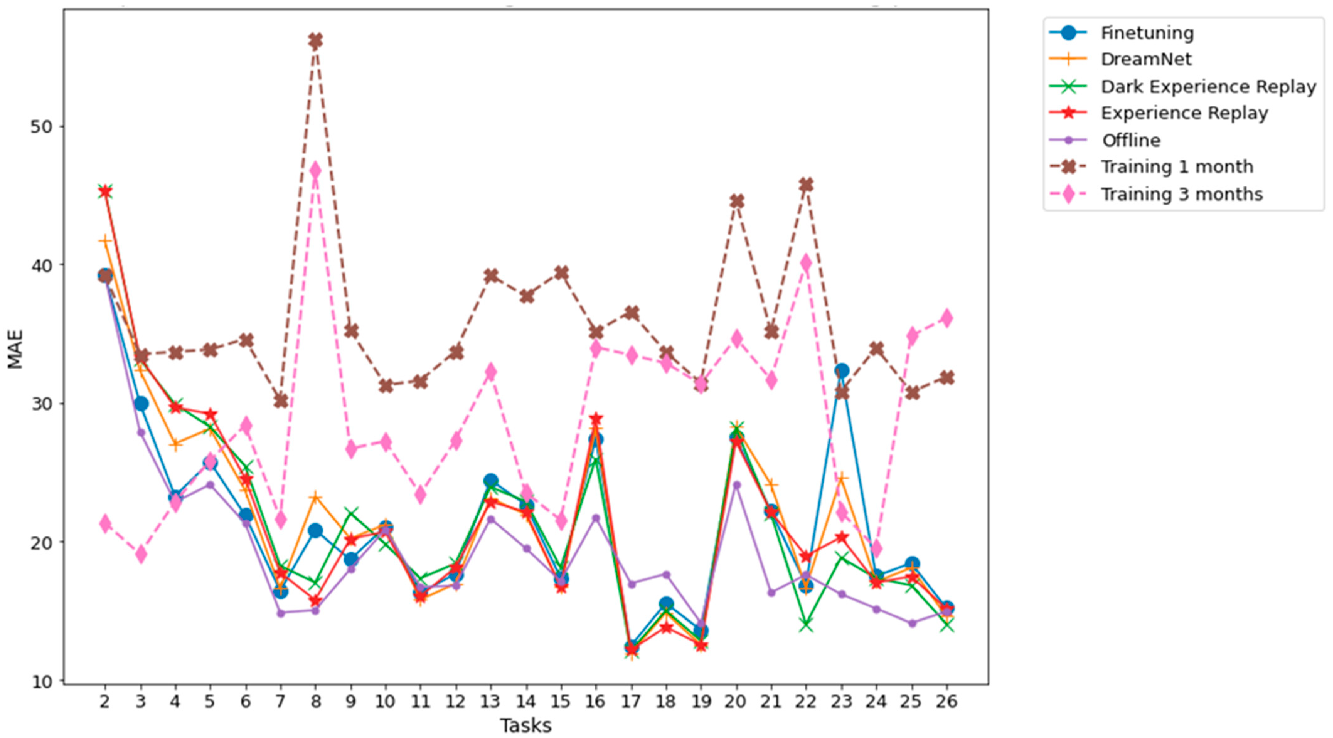
Figure 7 and Figure 8, related to Dwelling A and Dwelling B, respectively, summarize the performance evolution during the learning of the different continual learning algorithms and the baselines. On those figures, we present the MAE between predictions at time horizons 0.5 h, 1 h, 2 h, 6 h, 12 h, 18 h, and 24 h and their associated ground truth for each task, knowing that the model has been updated only with the previous task data, according to a given continual learning strategy. For example, MAE calculations between predictions and ground truth evaluation on task 3, are performed using a model that has been updated with task 1 data and then, without access to task 1 data, with task 2 data. Such a scenario is the most realistic and the most difficult: from a stream of data with potential shifts, we try to predict the future with access only to the last task. The results shown in Figure 7 and Figure 8 are obtained by averaging the MAE over five different runs. Standard deviations for the MAE on each task, associated with the five runs, are presented in Figure 9 and Figure 10.
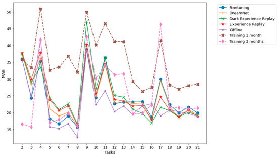
Figure 7.
Dwelling A MAE between multiple time horizon predictions and their associated ground truth for each task. The prediction time horizons are 0.5 h, 1 h, 2 h, 6 h, 12 h, 18 h, 24 h. The results shown are obtained from an average of 5 runs.
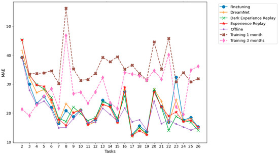
Figure 8.
Dwelling B MAE between multiple time horizon predictions and their associated ground truth for each task. The prediction time horizons are 0.5 h, 1 h, 2 h, 6 h, 12 h, 18 h, 24 h. The results shown are obtained from an average of 5 runs.
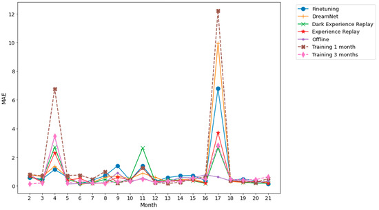
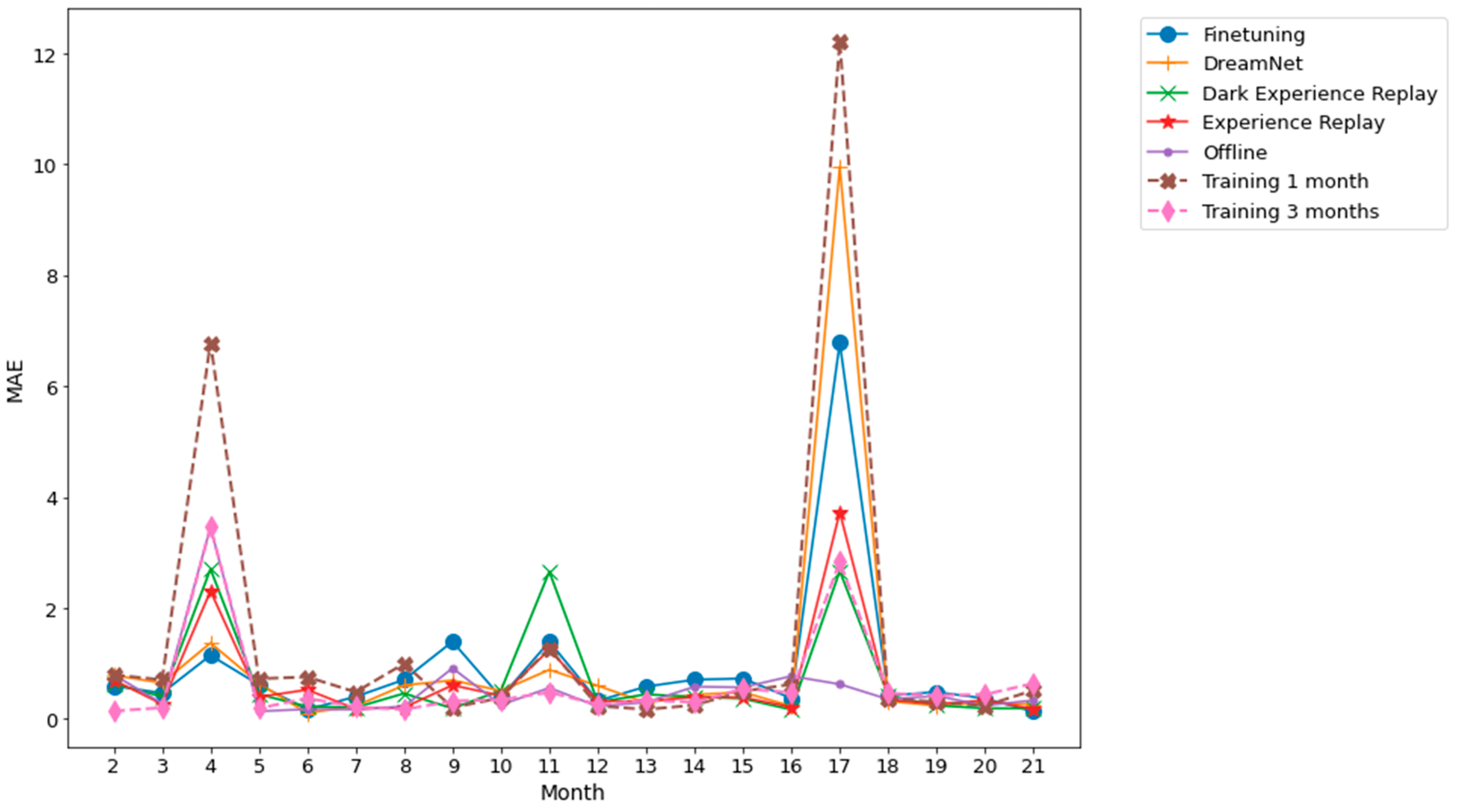
Figure 9.
Dwelling A standard deviation associated with the 5 runs whose mean is shown in Figure 7.
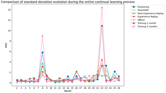
Figure 10.
Dwelling B standard deviation associated with the 5 runs whose mean is shown in Figure 8.
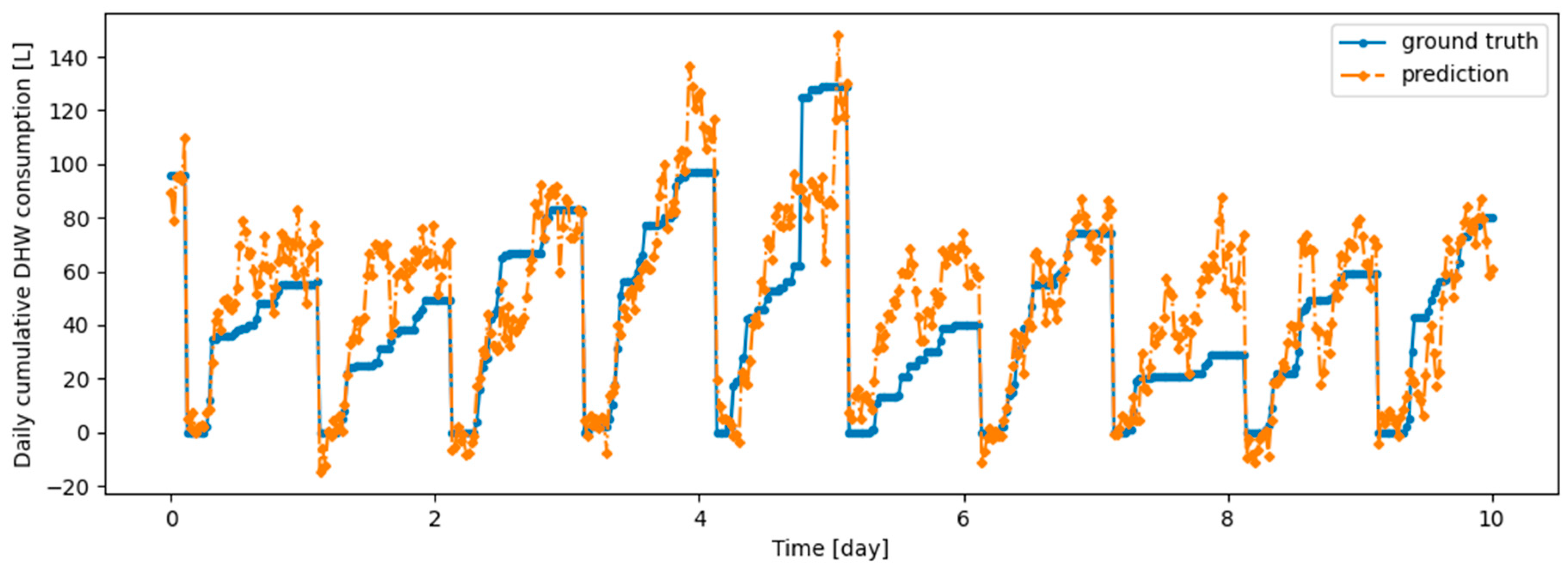
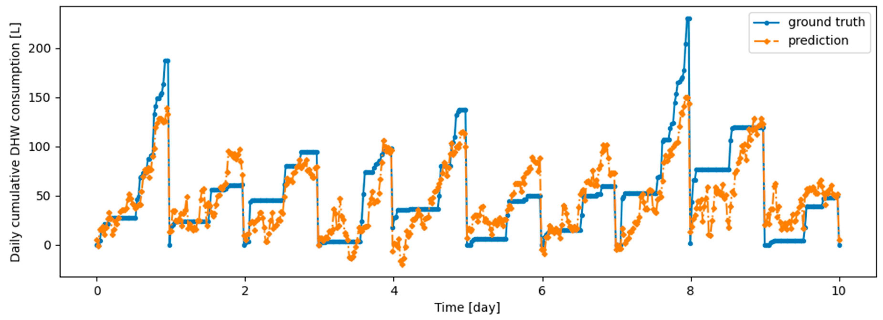
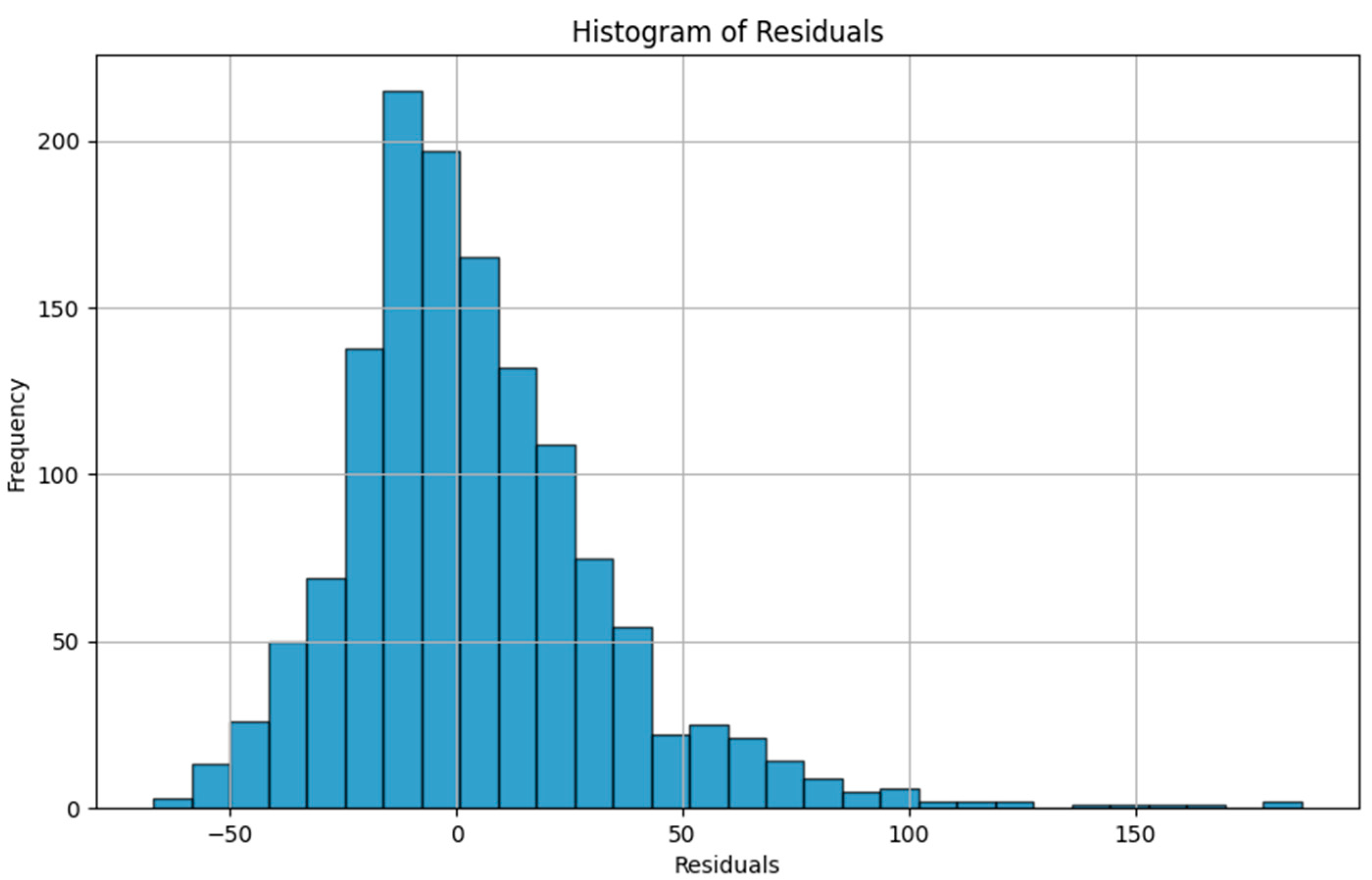
As an illustration of the prediction capability of the implemented models, we present a 6 h prediction against ground truth for Dream Net in Figure 11. The data presented in this section are taken from the last task of the time series of Dwelling A. The prediction model has learned continuously, i.e., task after task without accessing data from previous tasks, following the Dream Net algorithm on all but the last task. More examples of prediction versus ground truth comparisons for the different implemented algorithms are presented in Appendix A. Figure 12 is a residual plot associated with the last task of the Dwelling A dataset and continuous training over the previous tasks using the Dream Net algorithm. The presence of a few outliers associated with high consumption that are not correctly predicted can be noted. Apart from these outliers, where the predictions are underestimated, the residuals are balanced and concentrated around the zero axis, as can be seen in the corresponding histogram in Figure 13. Residual plots for other continual learning algorithms are provided in Appendix B.
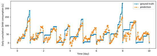
Figure 11.
Example of 6-h prediction versus ground truth for 10 days in the last task of Dwelling A’s DHW consumption with a model continuously trained with the Dream Net algorithm.
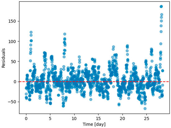
Figure 12.
Residual plot (ground truth minus predicted value) of the last task of Dwelling A DHW consumption with a model continuously trained with Dream Net with all tasks except the last one of Dwelling A.
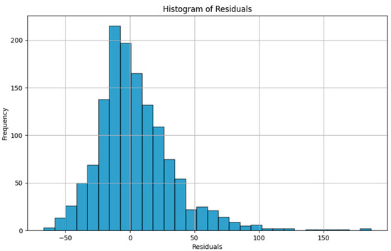
Figure 13.
Residual plot (ground truth minus predicted value) histogram of the last task of Dwelling A DHW consumption with a model continuously trained using the Dream Net algorithm with all tasks except the last one in Dwelling A.
The results averaged over all the tasks from the real DHW consumption of individual dwellings presented in Section 2.2 with Table 6 show that the average performances of each method are close to each other: on average, Finetuning performs slightly better than other methods, followed by Dream Net, DER and ER. The average performances of ER and DER are almost the same for both Dwelling A and Dwelling B data. On average, Dream Net performs better than DER and ER on Dwelling A data, while on average, DER and ER perform slightly better than Dream Net on Dwelling B data. The results in Table 6 show that 1-month and 3-month strategies, where the model is trained with the first month and the first three months, respectively, and then is not updated, are strongly outperformed by other continual learning algorithms, thus confirming the fact that the distribution of the data changes over time and that updating the model is necessary for the DHW datasets we are interested in.
Table 6.
Mean and standard deviation over all months (over the 5 runs) for the DHW consumption of Dwelling A and Dwelling B. The MAE is averaged for the difference prediction horizons.
3.3. Results for the Synthetic Dataset
In this section, we present the results of the experiment using synthetic datasets.
The hyperparameters for the MHA are the same as those used for the real dwelling, summarized in Table 3.
The hyperparameters used for the continual learning algorithms in this experiment are obtained via a grid search, as for real dwelling data. Tested and optimal hyperparameter values are presented in Table 7 and Table 8, respectively, for the Dream Net and the DER/ER algorithms. The optimality criterion for the hyperparameters is the sum of the MAE on d1_test and d2_test, respectively, plus the absolute value of the difference between these two MAEs. This optimality criterion has been chosen to select a configuration where both MAE on d1_test and d2_test are low and where a compromise between stability and plasticity is found. The number of epochs when finetuning the model without a continual learning algorithm is 70. This number of epochs is also used for the finetuning setup, where the model is updated without any continual learning method on d2_train after the initial learning on d1_train.
Table 7.
Hyperparameters tested in the grid search and optimal hyperparameters for the Dream Net algorithm.
Table 8.
Hyperparameters tested in the grid search and optimal hyperparameters for the DER and ER algorithms.
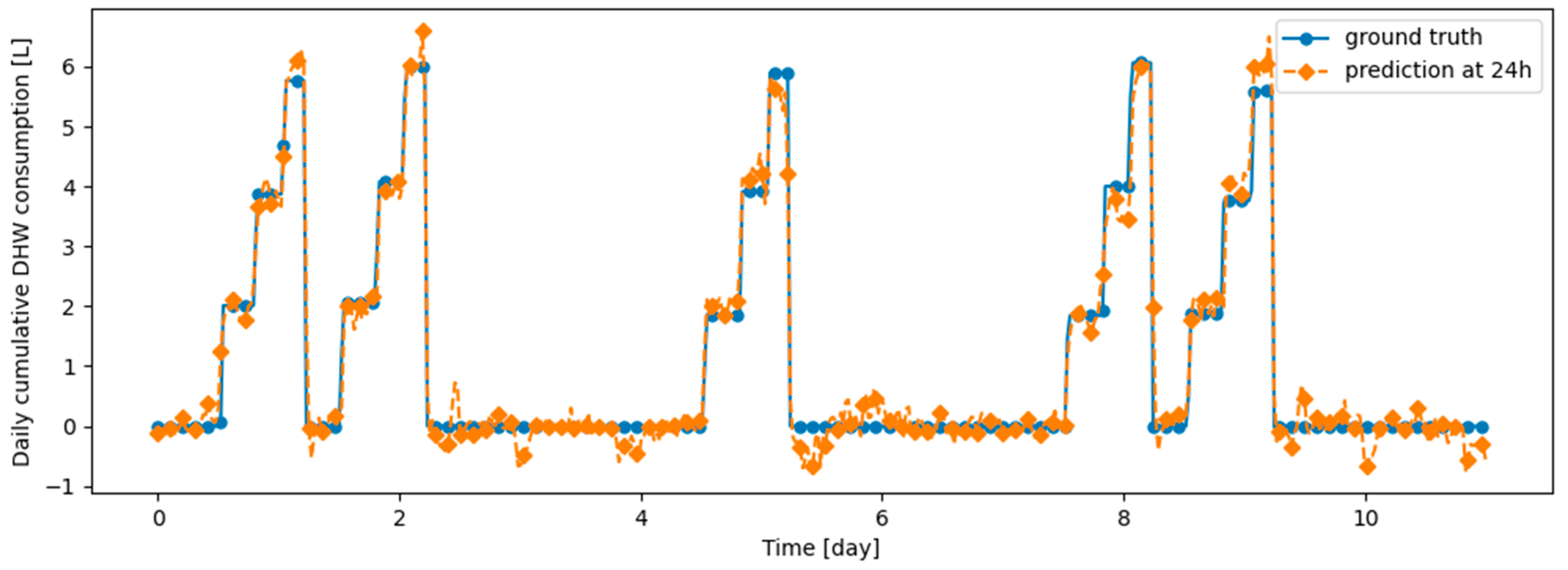
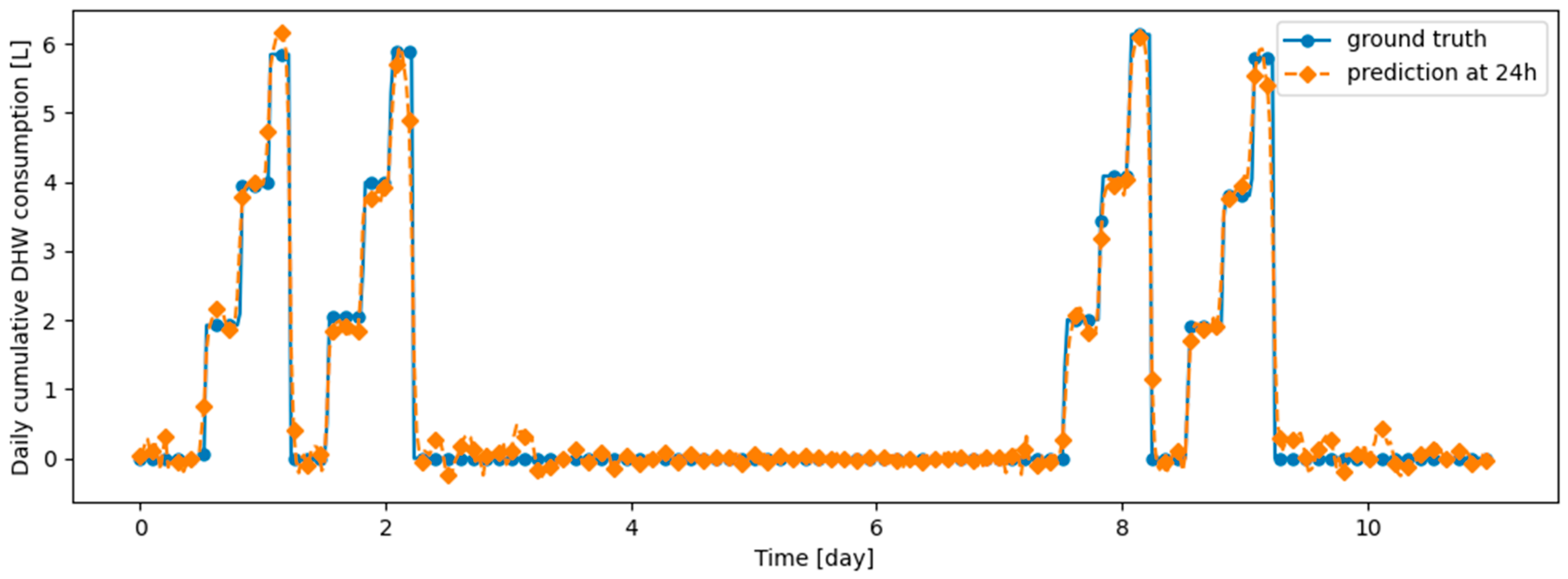
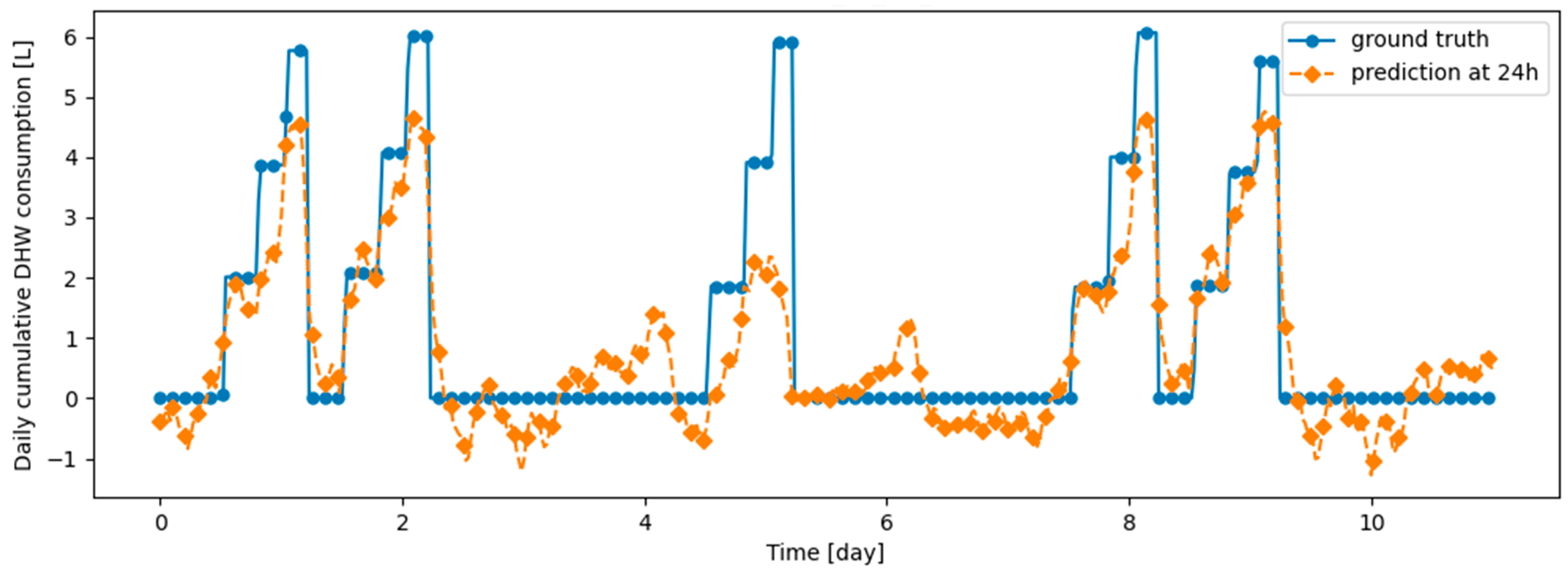
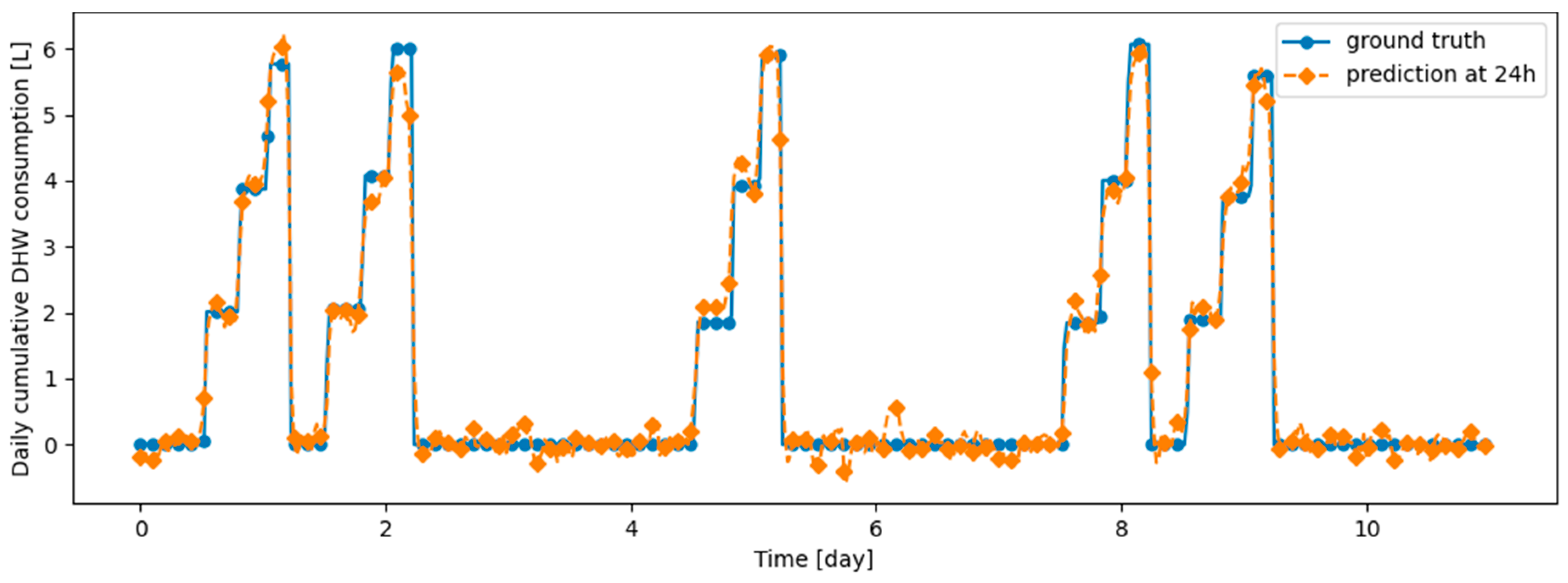
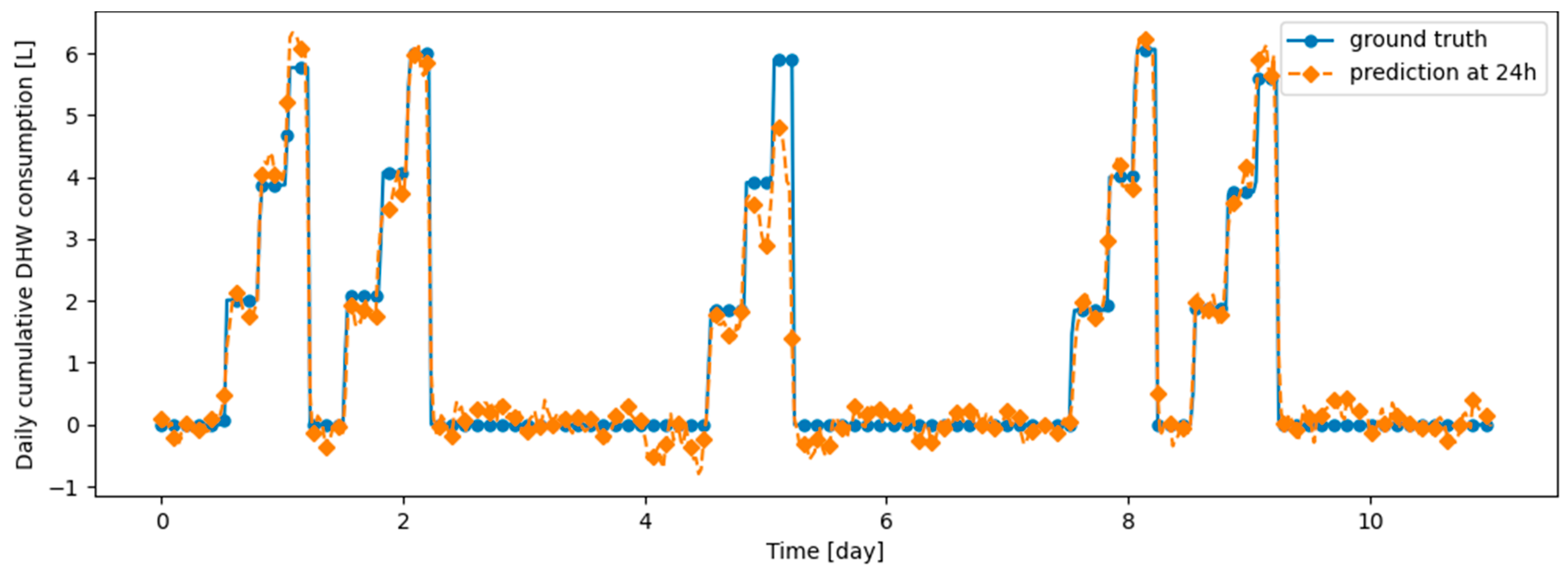
Table 9 summarizes the model performance without and with continual learning algorithms on the validation datasets, which are described in the remainder of this section. Before testing continual learning algorithms, we checked that training the model only on d1_train yields very poor prediction performance on d2_val, confirming that the model does not generalize naturally on d2_val. Figure 14 and Figure 15 illustrate the fact that, after learning d1_train, predictions on d1_val are made correctly, while those on d2_val are made poorly. We also checked that the prediction model has the ability to provide efficient prediction on both d1_val and d2_val when d1_train and d2_train are learned jointly: this confirms that the prediction model is able to correctly predict both types of data simultaneously. Finetuning the model on d2_train without continual learning algorithm, after learning d1_train, results in poor performance on d1_val, demonstrating the presence of catastrophic forgetting, as shown in Table 9, Figure 16 and Figure 17. Despite a loss of performance on both d1_val and d2_val, Dream Net provides balanced performance and mitigates catastrophic forgetting. An example of prediction, respectively on d1_val and d2_val, after learning d2_train using Dream Net versus ground truth is provided in Figure 18 and Figure 19. DER and ER allow a significant increase in the stability of the model, while hardly hindering the learning on d2_val. Examples of prediction versus ground truth associated with those models are provided in Appendix B. On the synthetic learning scenario built, DER gives the best performance. However, unlike Dream Net, DER requires the storage of real examples, which may compromise privacy. Finally, we note that for all the simulations performed, the standard deviations for both MAE on d1_val, d2_val, d1_test and d2_test are small compared to the MAE, implying that the training does not critically depend on the initialization state of the model.
Table 9.
MAE and associated standard deviation over 5 runs on synthetic validation data, after learning d1_train and updating the model with a continual learning algorithm or finetuning it on d2_train. The MAE and associated standard deviation on the joint learning setup, where d1_train and d2_train are learned simultaneously, are also shown.
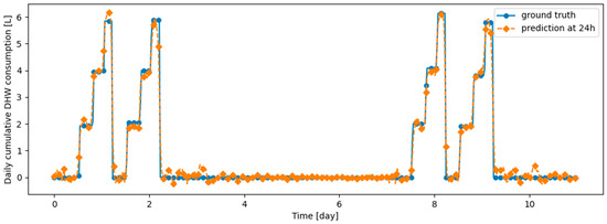
Figure 14.
Example of 24-h prediction versus ground truth for 11 days of d1_test, after training the model on d1_train.
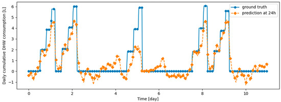
Figure 15.
Example of 24-h prediction versus ground truth for 11 days of d2_test, after training the model on d1_train.
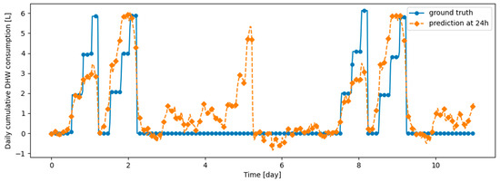
Figure 16.
Example of 24-h prediction versus ground truth for 11 days of d1_test, after first training the model on d1_train and then finetuning the model on d2_train, with no particular continual learning strategy.
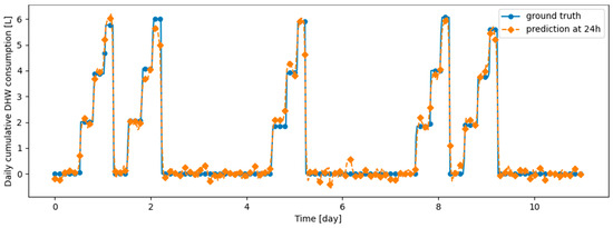
Figure 17.
Example of 24-h prediction versus ground truth for 11 days of d2_test, after first training the model on first d1_train and then finetuning the model on d2_train, with no particular continual learning strategy.
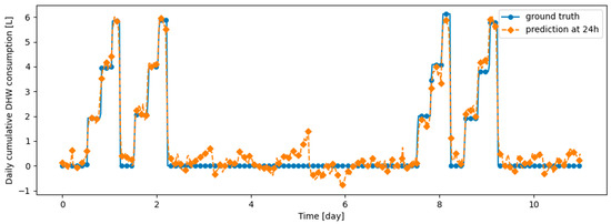
Figure 18.
Example of 24-h prediction versus ground truth for 11 days of d1_test, after training the model first on d1_train and then on d2_train using Dream Net.

Figure 19.
Example of 24-h prediction versus ground truth for 11 days of d2_test, after training the model first on d1_train and then on d2_train using Dream Net.
Table 10 summarizes the performances of the models on the test datasets. We have checked that the best hyperparameters for the different methods are the same as those described in Table 7 and Table 8. The comparison between the performances on the validation and test datasets shows a very small difference, thus confirming that the prediction model and continual learning methods generalize well to data from the same distribution that were not used for training or for setting the hyperparameters.
Table 10.
MAE and associated standard deviation over 5 runs on synthetic test data, after learning d1_train and updating the model with a continual learning algorithm or finetuning it on d2_train. The MAE and associated standard deviation on the joint learning setup, where d1_train and d2_train are learned simultaneously, are also shown.
4. Discussion
In the case of real dwellings, beyond the apparent similarity of the performance of the different continual learning algorithms and looking at the prediction quality task by task, Figure 7 and Figure 8 show that for two given tasks, the continual learning algorithm associated with the best prediction can be different. For example, in Figure 7, associated with Dwelling A, Finetuning significantly outperforms other algorithms for task 3, while DER outperforms other algorithms, especially Finetuning, for task 4. Moreover, the offline setting is the upper bound of accuracy—at the cost of an unlimited memory budget—for all continual learning strategies, since in this strategy all previously seen data are learned again. Nevertheless, in Figure 7 and 8, the offline setting yields accuracies for some tasks that are below those of the continual learning algorithms and even below or at the same level as Finetuning; see, for example, task 22 of Dwelling B. We explain this difference by the fact that, as the time series distribution shifts, previously seen knowledge may contradict recently seen knowledge. Such a finding shows that when searching for the best strategy to adapt a prediction algorithm to an evolving time series, prioritizing stability over plasticity is not always the optimal choice.
We want to emphasize the fact that the studied data from real dwellings are not associated with particular behaviors that would seem to require a continual learning algorithm. What we mean by this statement is that continual learning algorithms would seem to be particularly suitable for time series with alternating patterns: with such time series, the goal would be to continuously learn new patterns while not forgetting the previous ones, that are likely to reappear later. Nevertheless, our work shows that static models, where only the first month or first three months are learned without further updating, are largely outperformed by all implemented updating strategies. This finding suggests that model updating is necessary in this setting.
We also note that Figure 11 and other prediction examples given in Appendix A show that the implemented algorithms have qualitatively good prediction ability, with a large part of the peaks well predicted despite some missed, underestimated or overestimated consumption. This confirms that the prediction model based on multi-head attention is relevant for the prediction of DHW consumption.
As mentioned in Section 2.3, we design a synthetic dataset to evaluate the performance of continual learning algorithms in the case where the model has to learn sequentially two tasks, each associated with different regular patterns. These synthetic datasets are very important to understand the resilience of the different models in the face of a drastic change in the behavior of the residents (e.g., job change, move, vacation). Note that this case is a simplified version of the realistic case of two people with different habits successively occupying the same dwelling; it answers the question of whether the habits of the first person can still be predicted by the model after the model has learned the habits of the second person. The results associated with this experiment clearly demonstrate the interest of the continual learning method when periodic behavior occurs. This finding reinforces the idea that continual learning algorithms are very important to ensure reliable prediction performance for DHW consumption.
A future research direction is to apply the same strategies to other DHW consumption datasets: in particular, having datasets longer than two years would help to determine if continual learning algorithms help to achieve better performance at longer time scales; having real dwelling datasets containing different regular patterns that occasionally reappear, for example, associated with residents having a particular work schedule, would allow to measure the gain associated with continual learning algorithms in a real case. Future work directions also include the testing of other continual learning strategies implemented for the prediction of DHW consumption; in the field of computer vision, Transformers adapted to be continual learners, such as BiRT [29], have been developed, implementing such modified transformers and applying them to time series prediction, and especially the prediction of DHW consumption seems to us as a promising direction. Finally, Dream Net, in the case of synthetic data, despite having the advantage of preserving privacy, gives performances that are decent but lower than those of DER and ER; such a difference was not expected since, for classification, Dream Net gives strong performance compared to other buffer-based methods [27]. This difference could be due to the use of multi-head attention instead of dense layers: this change could affect the noise injection step used to extract knowledge from the Memory Net. Further research would be needed to investigate this point and possibly adapt Dream Net to multi-head attention.
5. Conclusions
We have addressed the problem of time series forecasting applied to the prediction of DHW consumption associated with a nonstationary data stream, first in the realistic case where we have continuously trained a prediction model on the previous tasks and predicted the consumption of the next task, then in a special case with physically plausible synthetic data that we have generated to determine the potential performance improvement of continual learning algorithms in the case of abrupt changes in the data distribution. The main conclusions of our work are:
- The implemented continual learning algorithms, Experience Replay, Dark Experience Replay and Dream Net, can tackle catastrophic forgetting for prediction models based on transformers.
- Successively learning tasks from the two studied real dwellings data shows the importance of updating the model during the use of the prediction model.
- No update strategy is consistently better than the other with the real DHW consumption data we have: even the offline setting, which uses all previously seen data to predict the next task, can be outperformed by other strategies. This suggests the counterintuitive fact that a high degree of model stability can, in some cases, reduce time series forecasting performance.
- Continual learning algorithms significantly improve prediction performance when brutal changes occur, as demonstrated in the case of the synthetic dataset, which implements two separate patterns learned sequentially.
Author Contributions
Conceptualization, R.B., M.R., A.L. and M.M.; methodology, R.B., M.R., A.L. and M.M.; software, R.B. and V.C.; validation, R.B., M.R., A.L. and M.M.; investigation, R.B., M.R., A.L. and M.M.; data curation, R.B. and A.L.; writing—original draft preparation, R.B.; writing—review and editing, R.B., M.R., A.L. and M.M.; visualization, R.B. and V.C.; supervision, M.R. and M.M.; project administration, M.R. and M.M.; funding acquisition, M.R. and M.M. All authors have read and agreed to the published version of the manuscript.
Funding
This work was both funded by a public grant overseen by the French National Research Agency (ANR) as part of the ‘AAP MESRI—BMBF en Intelligence Artificielle_ AI4HP ANR-21-FAI2-0006-02’ and by MIAI @ Grenoble Alpes (ANR-19-P3IA-0003).
Data Availability Statement
The data and code developed during this research work are the properties of Commissariat à l‘énergie atomique et aux énergies alternatives and cannot be shared publicly.
Acknowledgments
Some data and algorithmic resources used in this work come from output materials of the European Union’s Seventh Framework Program FP7/2007-2011 under grant agreement n° 282825 –AcronymMacSheep.
Conflicts of Interest
The authors declare no conflicts of interest. The funders had no role in the design of the study; in the collection, analyses, or interpretation of data; in the writing of the manuscript; or in the decision to publish the results.
Appendix A
This appendix presents examples of prediction versus ground truth for 10 days in the last task of data from real DHW consumption, respectively from Dwelling A and Dwelling B with models continuously trained, respectively, with DER, ER, Dream Net, Finetuning and Offline algorithms.
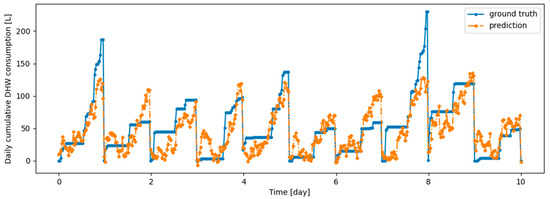
Figure A1.
Example of 6 h prediction versus ground truth for 10 days in the last task of Dwelling A DHW consumption with a model continuously trained with DER algorithm.
Figure A1.
Example of 6 h prediction versus ground truth for 10 days in the last task of Dwelling A DHW consumption with a model continuously trained with DER algorithm.


Figure A2.
Example of 6 h prediction versus ground truth for 10 days in the last task of Dwelling A DHW consumption with a model continuously trained with ER algorithm.
Figure A2.
Example of 6 h prediction versus ground truth for 10 days in the last task of Dwelling A DHW consumption with a model continuously trained with ER algorithm.
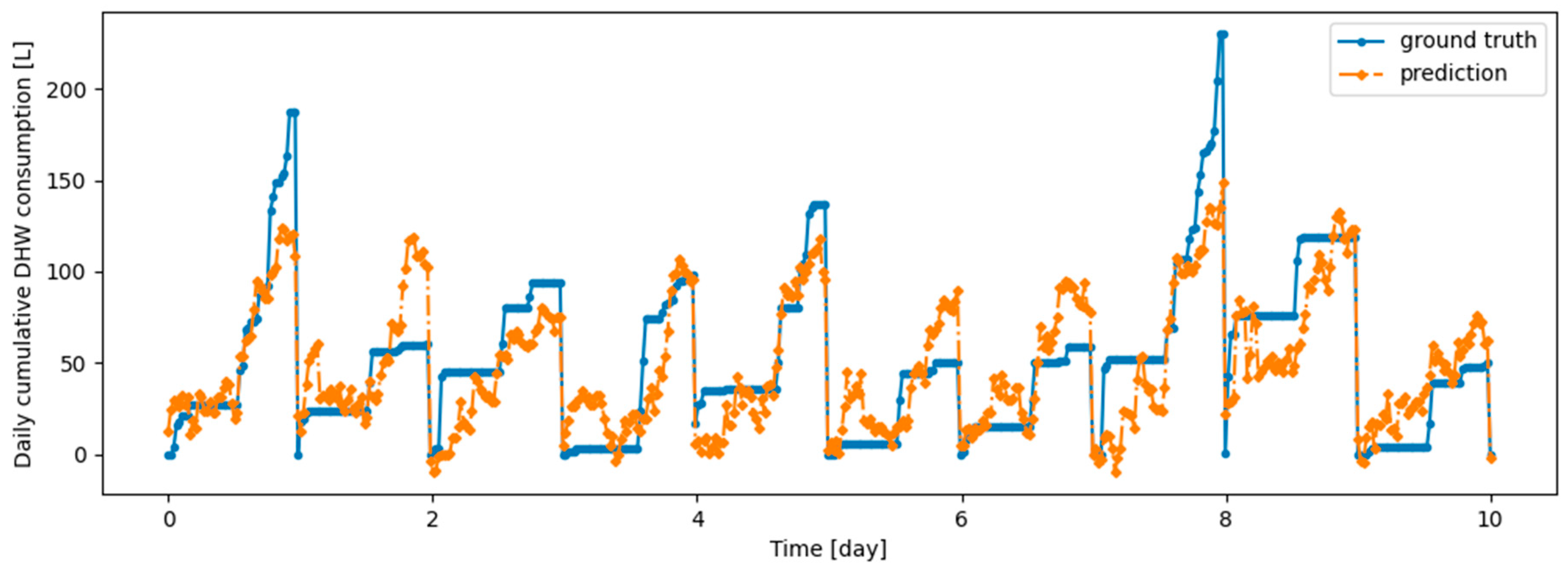

Figure A3.
Example of 6 h prediction versus ground truth for 10 days in the last task of Dwelling A DHW consumption with a model continuously trained with finetuning setup.
Figure A3.
Example of 6 h prediction versus ground truth for 10 days in the last task of Dwelling A DHW consumption with a model continuously trained with finetuning setup.
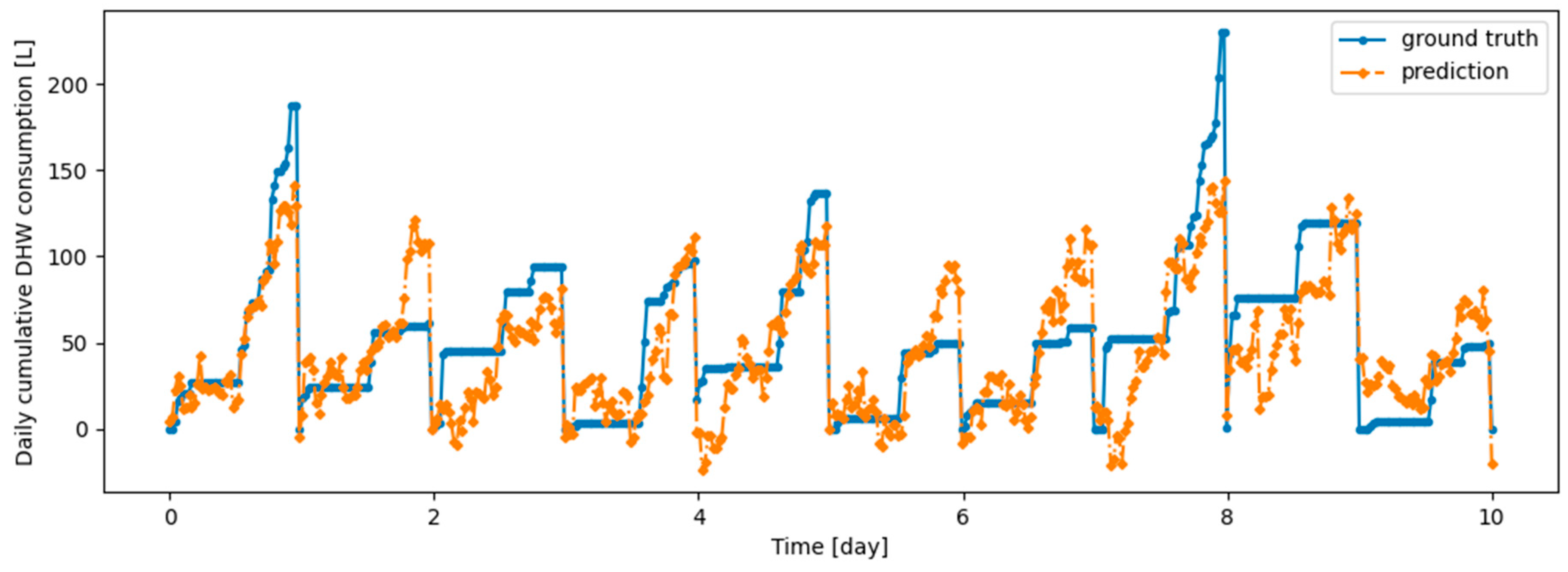
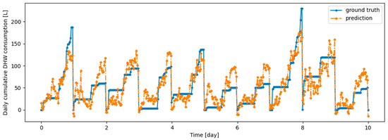
Figure A4.
Example of 6 h prediction versus ground truth for 10 days in the last task of Dwelling A DHW consumption with a model continuously trained with offline setup.
Figure A4.
Example of 6 h prediction versus ground truth for 10 days in the last task of Dwelling A DHW consumption with a model continuously trained with offline setup.
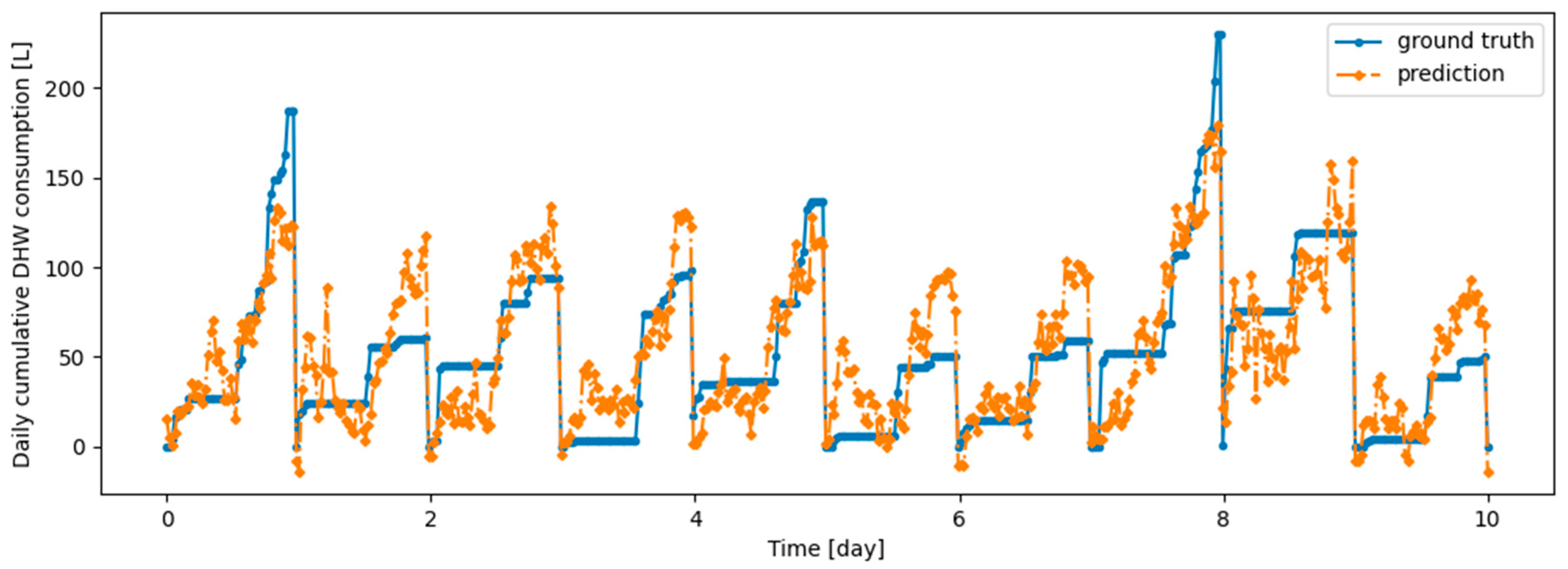
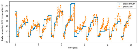
Figure A5.
Example of 6 h prediction versus ground truth for 10 days in the last task of Dwelling B DHW consumption with a model continuously trained with DER algorithm.
Figure A5.
Example of 6 h prediction versus ground truth for 10 days in the last task of Dwelling B DHW consumption with a model continuously trained with DER algorithm.

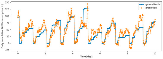
Figure A6.
Example of 6 h prediction versus ground truth for 10 days in the last task of Dwelling B DHW consumption with a model continuously trained with ER algorithm.
Figure A6.
Example of 6 h prediction versus ground truth for 10 days in the last task of Dwelling B DHW consumption with a model continuously trained with ER algorithm.
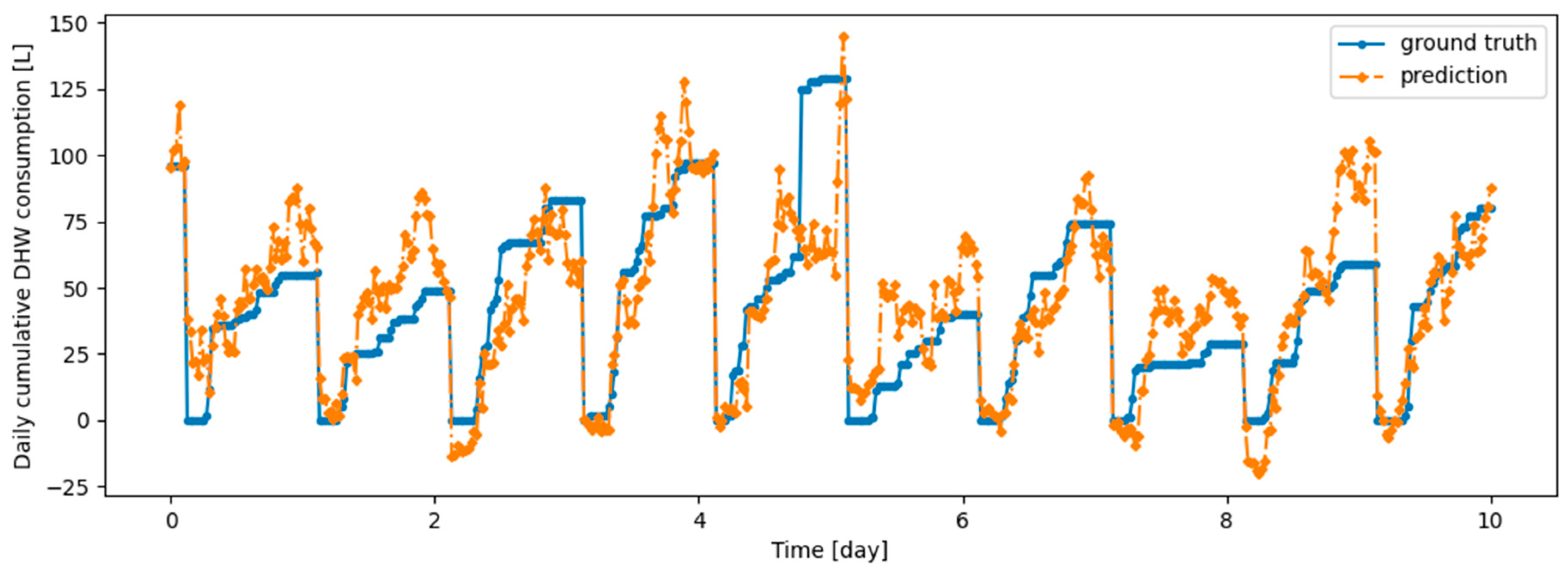

Figure A7.
Example of 6 h prediction versus ground truth for 10 days in the last task of Dwelling B DHW consumption with a model continuously trained with Dream Net algorithm.
Figure A7.
Example of 6 h prediction versus ground truth for 10 days in the last task of Dwelling B DHW consumption with a model continuously trained with Dream Net algorithm.
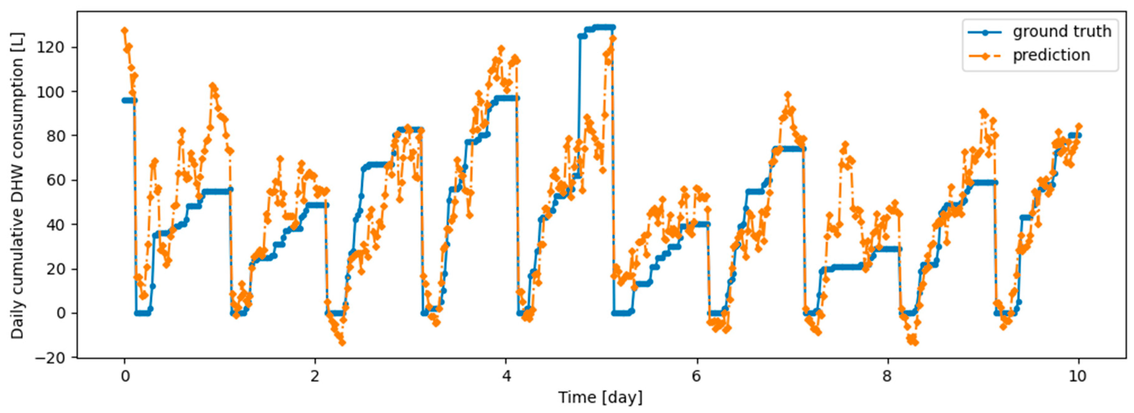
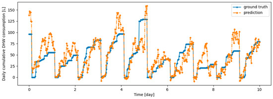
Figure A8.
Example of 6 h prediction versus ground truth for 10 days in the last task of Dwelling B DHW consumption with a model continuously trained with the Finetuning setup.
Figure A8.
Example of 6 h prediction versus ground truth for 10 days in the last task of Dwelling B DHW consumption with a model continuously trained with the Finetuning setup.
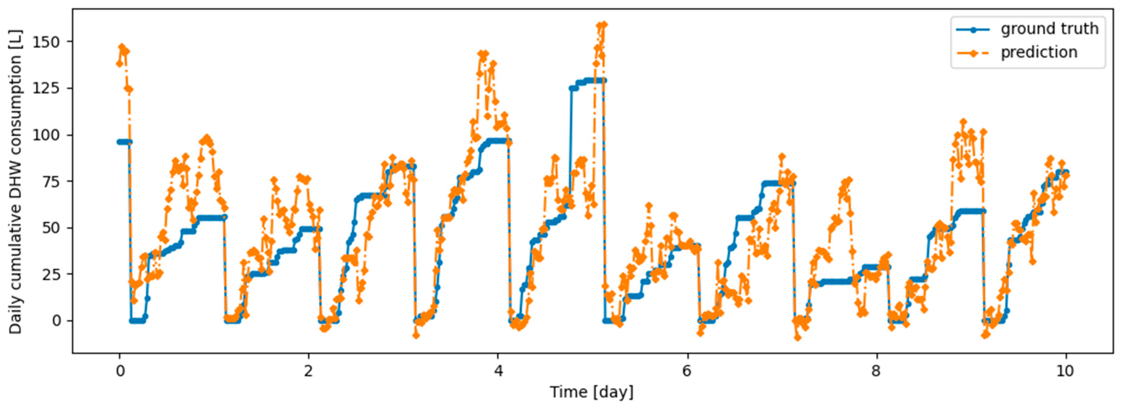
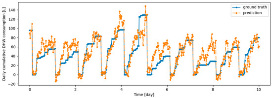
Figure A9.
Example of 6 h prediction versus ground truth for 10 days in the last task of Dwelling B DHW consumption with a model continuously trained with the offline setup.
Figure A9.
Example of 6 h prediction versus ground truth for 10 days in the last task of Dwelling B DHW consumption with a model continuously trained with the offline setup.
Appendix B
This appendix presents residual plots (ground truth value minus 6 h predicted value) of the last task of Dwelling A DHW consumption with models continuously trained with every task except the last one in Dwelling A.

Figure A10.
Residual plots (ground truth value minus 6 h predicted value) of the last task of Dwelling A DHW consumption with models continuously trained with DER with every task except the last one in Dwelling A.
Figure A10.
Residual plots (ground truth value minus 6 h predicted value) of the last task of Dwelling A DHW consumption with models continuously trained with DER with every task except the last one in Dwelling A.

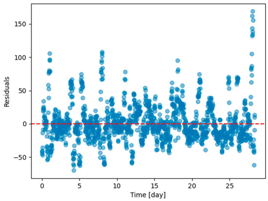
Figure A11.
Residual plots (ground truth value minus 6 h predicted value) of the last task of Dwelling A DHW consumption with models continuously trained with ER with every task except the last one in Dwelling A.
Figure A11.
Residual plots (ground truth value minus 6 h predicted value) of the last task of Dwelling A DHW consumption with models continuously trained with ER with every task except the last one in Dwelling A.


Figure A12.
Residual plots (ground truth value minus 6 h predicted value) of the last task of Dwelling A DHW consumption with models continuously trained with finetuning setting with every task except the last one in Dwelling A.
Figure A12.
Residual plots (ground truth value minus 6 h predicted value) of the last task of Dwelling A DHW consumption with models continuously trained with finetuning setting with every task except the last one in Dwelling A.

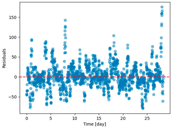
Figure A13.
Residual plots (ground truth value minus 6 h predicted value) of the last task of Dwelling A DHW consumption with models continuously trained with offline setting with every task except the last one in Dwelling A.
Figure A13.
Residual plots (ground truth value minus 6 h predicted value) of the last task of Dwelling A DHW consumption with models continuously trained with offline setting with every task except the last one in Dwelling A.

Appendix C
This appendix presents examples of prediction versus ground truth for 11 days in either d1_test or d2_test with DER and ER algorithms.
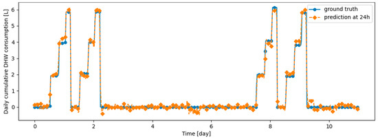
Figure A14.
Example of 24 h prediction versus ground truth for 11 days of d1_test, after the model has been initially trained on d1_train and then learned d2_train using ER.
Figure A14.
Example of 24 h prediction versus ground truth for 11 days of d1_test, after the model has been initially trained on d1_train and then learned d2_train using ER.
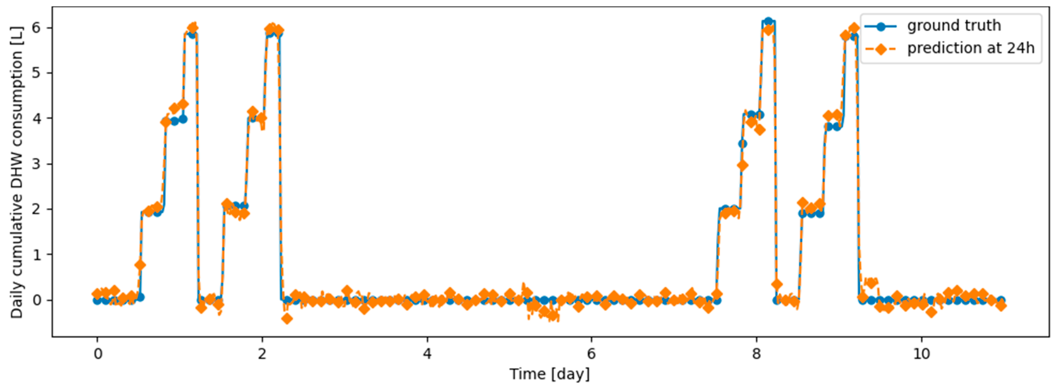
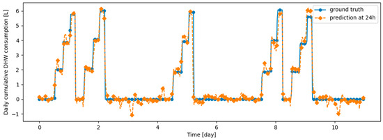
Figure A15.
Example of 24 h prediction versus ground truth for 11 days of d2_test, after the model has been initially trained on d1_train and then learned d2_train using ER.
Figure A15.
Example of 24 h prediction versus ground truth for 11 days of d2_test, after the model has been initially trained on d1_train and then learned d2_train using ER.
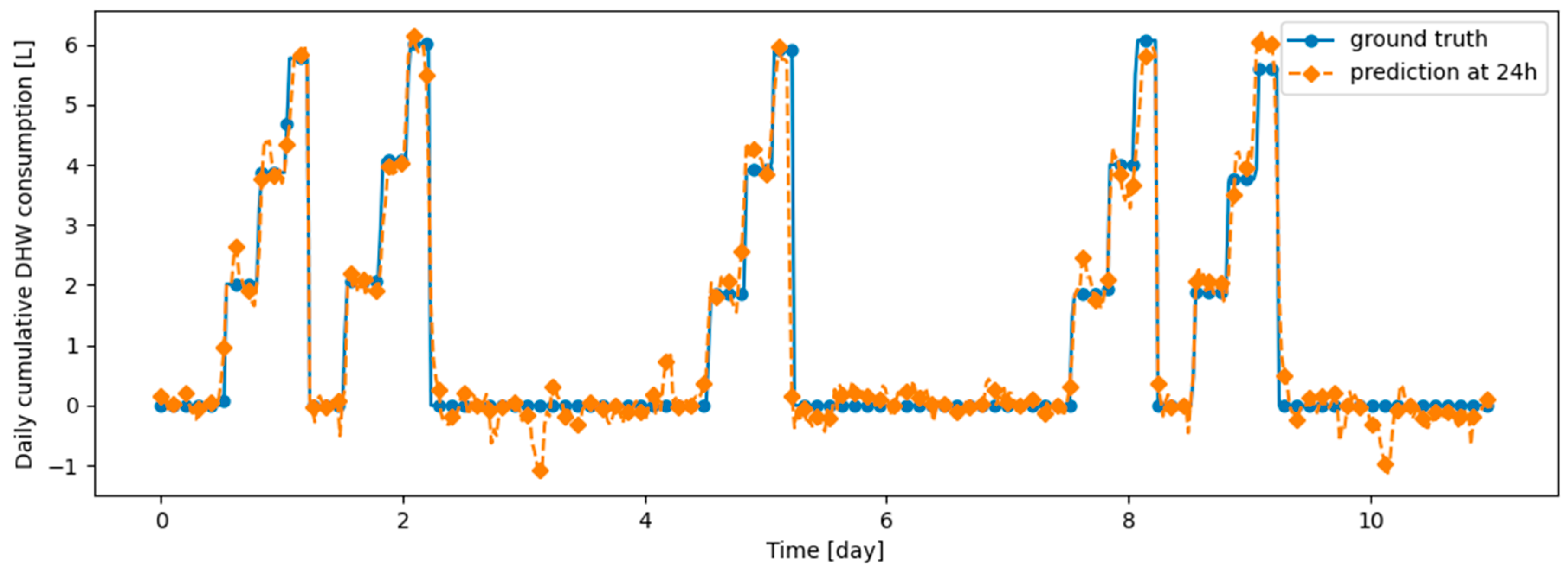
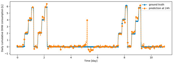
Figure A16.
Example of 24 h prediction versus ground truth for 11 days of d1_test, after the model has been initially trained on d1_train and then learned d2_train using DER.
Figure A16.
Example of 24 h prediction versus ground truth for 11 days of d1_test, after the model has been initially trained on d1_train and then learned d2_train using DER.
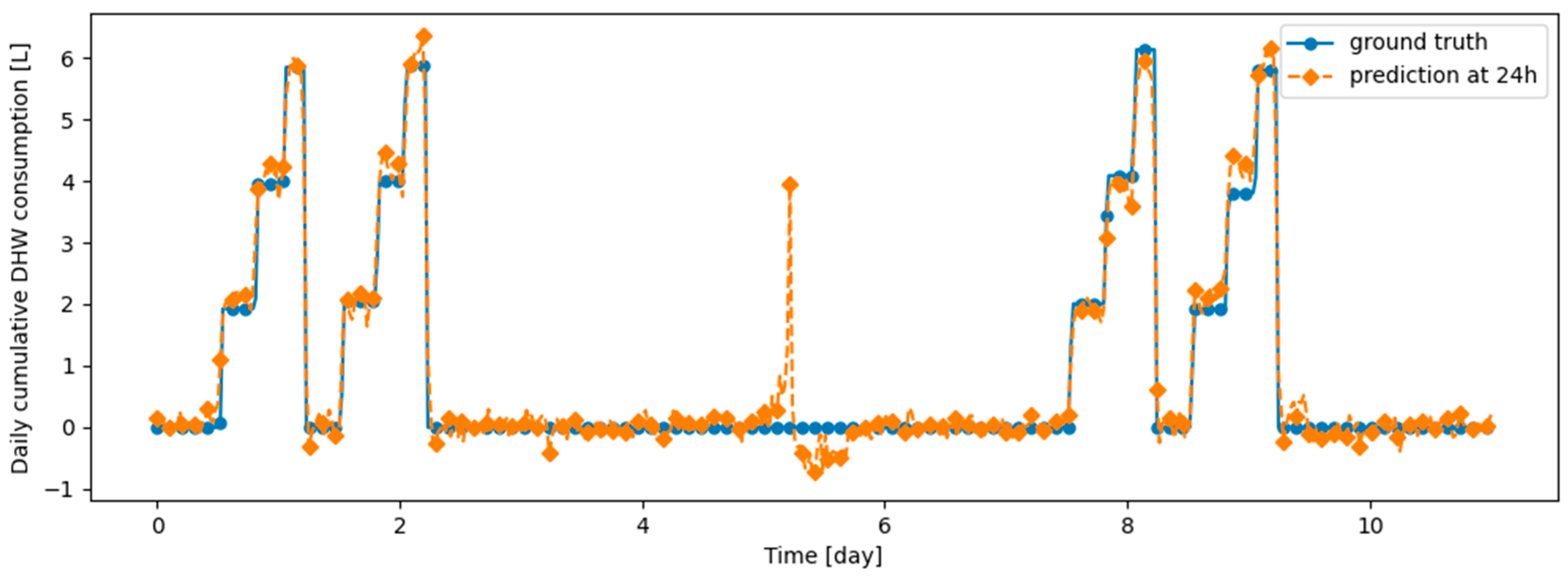
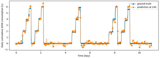
Figure A17.
Example of 24 h prediction versus ground truth for 11 days of d2_test, after the model has been initially trained on d1_train and then learned d2_train using DER.
Figure A17.
Example of 24 h prediction versus ground truth for 11 days of d2_test, after the model has been initially trained on d1_train and then learned d2_train using DER.
References
- Mainsant, M.; Solinas, M.; Reyboz, M.; Godin, C.; Mermillod, M. Dream Net: A Privacy Preserving Continual Learning Model for Face Emotion Recognition. In Proceedings of the 9th International Conference on Affective Computing and Intelligent Interaction Workshops and Demos (ACIIW), Nara, Japan, 28 September–1 October 2021. [Google Scholar]
- Hoang Vuong, P.; Tan Dat, T.; Khoi Mai, T.; Hoang Uyen, P.; The Bao, P. Stock-Price Forecasting Based on XGBoost and LSTM. Comput. Syst. Sci. Eng. 2022, 40, 237–246. [Google Scholar] [CrossRef]
- Zhang, L.; Bian, W.; Qu, W.; Tuo, L.; Wang, Y. Time Series Forecast of Sales Volume Based on XGBoost. J. Phys. Conf. Ser. 2021, 1873, 012067. [Google Scholar] [CrossRef]
- Liu, Z.; Wu, D.; Liu, Y.; Han, Z.; Lun, L.; Gao, J.; Jin, G.; Cao, G. Accuracy Analyses and Model Comparison of Machine Learning Adopted in Building Energy Consumption Prediction. Energy Explor. Exploit. 2019, 37, 1426–1451. [Google Scholar] [CrossRef]
- Lomet, A.; Suard, F.; Chèze, D. Statistical Modeling for Real Domestic Hot Water Consumption Forecasting. Energy Procedia 2015, 70, 379–387. [Google Scholar] [CrossRef]
- Hochreiter, S.; Schmidhuber, J. Long Short-Term Memory. Neural Comput. 1997, 9, 1735–1780. [Google Scholar] [CrossRef]
- Chung, J.; Gulcehre, C.; Cho, K.; Bengio, Y. Empirical Evaluation of Gated Recurrent Neural Networks on Sequence Modeling. arXiv 2014, arXiv:1412.3555. [Google Scholar]
- Lipton, Z.C.; Berkowitz, J.; Elkan, C. A Critical Review of Recurrent Neural Networks for Sequence Learning. arXiv 2015, arXiv:1506.00019. [Google Scholar]
- Koprinska, I.; Wu, D.; Wang, Z. Convolutional Neural Networks for Energy Time Series Forecasting. In Proceedings of the 2018 International Joint Conference on Neural Networks (IJCNN), Rio de Janeiro, Brazil, 8–13 July 2018; pp. 1–8. [Google Scholar]
- Wang, K.; Li, K.; Zhou, L.; Hu, Y.; Cheng, Z.; Liu, J.; Chen, C. Multiple Convolutional Neural Networks for Multivariate Time Series Prediction. Neurocomputing 2019, 360, 107–119. [Google Scholar] [CrossRef]
- Vaswani, A.; Shazeer, N.; Parmar, N.; Uszkoreit, J.; Jones, L.; Gomez, A.N.; Kaiser, L.; Polosukhin, I. Attention Is All You Need. arXiv 2017, arXiv:1706.03762. [Google Scholar]
- Khan, S.; Naseer, M.; Hayat, M.; Zamir, S.W.; Khan, F.S.; Shah, M. Transformers in Vision: A Survey. ACM Comput. Surv. 2022, 54, 1–41. [Google Scholar] [CrossRef]
- Ahmed, S.; Nielsen, I.E.; Tripathi, A.; Siddiqui, S.; Ramachandran, R.P.; Rasool, G. Transformers in Time-Series Analysis: A Tutorial. Circuits Syst. Signal Process. 2023, 42, 7433–7466. [Google Scholar] [CrossRef]
- Wen, Q.; Zhou, T.; Zhang, C.; Chen, W.; Ma, Z.; Yan, J.; Sun, L. Transformers in Time Series: A Survey. arXiv 2023, arXiv:2202.07125. [Google Scholar]
- Compagnon, P.; Lomet, A.; Reyboz, M.; Mermillod, M. Domestic Hot Water Forecasting for Individual Housing with Deep Learning. In Machine Learning and Principles and Practice of Knowledge Discovery in Databases; Koprinska, I., Mignone, P., Guidotti, R., Jaroszewicz, S., Fröning, H., Gullo, F., Ferreira, P.M., Roqueiro, D., Ceddia, G., Nowaczyk, S., et al., Eds.; Communications in Computer and Information Science; Springer Nature: Cham, Switzerland, 2023; Volume 1753, pp. 223–235. ISBN 978-3-031-23632-7. [Google Scholar]
- French, R.M. Catastrophic Forgetting in Connectionist Networks. Trends Cogn. Sci. 1999, 3, 128–135. [Google Scholar] [CrossRef] [PubMed]
- van de Ven, G.M.; Tolias, A.S. Three Scenarios for Continual Learning. arXiv 2019, arXiv:1904.07734. [Google Scholar]
- Zeno, C.; Golan, I.; Hoffer, E.; Soudry, D. Task Agnostic Continual Learning Using Online Variational Bayes. arXiv 2019, arXiv:1803.10123. [Google Scholar]
- De Lange, M.; Aljundi, R.; Masana, M.; Parisot, S.; Jia, X.; Leonardis, A.; Slabaugh, G.; Tuytelaars, T. A Continual Learning Survey: Defying Forgetting in Classification Tasks. IEEE Trans. Pattern Anal. Mach. Intell. 2021, 44, 3366–3385. [Google Scholar] [CrossRef]
- Rusu, A.A.; Rabinowitz, N.C.; Desjardins, G.; Soyer, H.; Kirkpatrick, J.; Kavukcuoglu, K.; Pascanu, R.; Hadsell, R. Progressive Neural Networks. arXiv 2022, arXiv:1606.04671. [Google Scholar]
- Kirkpatrick, J.; Pascanu, R.; Rabinowitz, N.; Veness, J.; Desjardins, G.; Rusu, A.A.; Milan, K.; Quan, J.; Ramalho, T.; Grabska-Barwinska, A.; et al. Overcoming Catastrophic Forgetting in Neural Networks. Proc. Natl. Acad. Sci. USA 2017, 114, 3521–3526. [Google Scholar] [CrossRef]
- Bagus, B.; Gepperth, A. An Investigation of Replay-Based Approaches for Continual Learning. In Proceedings of the 2021 International Joint Conference on Neural Networks (IJCNN), Shenzhen, China, 18–22 July 2021; pp. 1–9. [Google Scholar]
- Rolnick, D.; Ahuja, A.; Schwarz, J.; Lillicrap, T.P.; Wayne, G. Experience Replay for Continual Learning. arXiv 2019, arXiv:1811.11682. [Google Scholar]
- Buzzega, P.; Boschini, M.; Porrello, A.; Abati, D.; Calderara, S. Dark Experience for General Continual Learning: A Strong, Simple Baseline. arXiv 2020, arXiv:2004.07211. [Google Scholar]
- Wang, L.; Zhang, X.; Su, H.; Zhu, J. A Comprehensive Survey of Continual Learning: Theory, Method and Application. arXiv 2024, arXiv:2302.00487. [Google Scholar] [CrossRef] [PubMed]
- Pham, Q.; Liu, C.; Sahoo, D.; Hoi, S.C.H. Learning Fast and Slow for Online Time Series Forecasting. arXiv 2022, arXiv:2202.11672. [Google Scholar]
- Mainsant, M.; Mermillod, M.; Godin, C.; Reyboz, M. A Study of the Dream Net Model Robustness across Continual Learning Scenarios. In Proceedings of the 2022 IEEE International Conference on Data Mining Workshops (ICDMW), Orlando, FL, USA, 28 November–1 December 2022; pp. 824–833. [Google Scholar]
- Li, K.-H. Reservoir-Sampling Algorithms of Time Complexity O (n (1 + log(N/n))). ACM Trans. Math. Softw. 1994, 20, 481–493. [Google Scholar] [CrossRef]
- Jeeveswaran, K.; Bhat, P.; Zonooz, B.; Arani, E. BiRT: Bio-Inspired Replay in Vision Transformers for Continual Learning. arXiv 2023, arXiv:2305.04769. [Google Scholar]


Disclaimer/Publisher’s Note: The statements, opinions and data contained in all publications are solely those of the individual author(s) and contributor(s) and not of MDPI and/or the editor(s). MDPI and/or the editor(s) disclaim responsibility for any injury to people or property resulting from any ideas, methods, instructions or products referred to in the content. |
© 2024 by the authors. Licensee MDPI, Basel, Switzerland. This article is an open access article distributed under the terms and conditions of the Creative Commons Attribution (CC BY) license (https://creativecommons.org/licenses/by/4.0/).