Abstract
As the world’s second-largest economy, China has experienced rapid industrialization and urbanization, resulting in high energy consumption and significant carbon emissions. This development has intensified conflicts between human-land relations and environmental conservation, contributing to global warming and urban air pollution, both of which pose serious health risks. This study uses nighttime light (NTL) data from 2005 to 2019, along with scaling techniques and statistical analysis, to estimate city-scale energy carbon emissions over a 15-year period. Focusing on Northeast China, a traditional industrial region comprising 36 cities across three provinces, we examine spatial patterns of energy carbon emissions and assess spatiotemporal evolution through spatial autocorrelation and dynamic changes. These changes are further evaluated using standard deviation ellipse (SDE) parameters and SLOPE values. Additionally, the Tapio decoupling index is applied to explore the relationship between city-scale emissions and economic growth. Our findings for the 36 cities over 15 years are: (1) Heilongjiang shows low, declining emissions; Jilin improves; Liaoning has high, steadily increasing emissions. (2) The global spatial autocorrelation of energy carbon emissions is significant, with a positive Moran’s I, while significant local Moran’s I clusters are concentrated in Heilongjiang and Liaoning. (3) The greatest emission changes occurred in 2015, followed by 2019, 2005, and 2010. (4) Emission growth is fastest in Heilongjiang, followed by Liaoning and Jilin. (5) Tapio analysis shows positive decoupling in Heilongjiang, declining decoupling in Jilin, and no change in Liaoning. This study provides a quantitative basis for dual carbon goals and offers emission reduction strategies for government, industry, and residents, supporting energy transition and sustainable urban planning.
1. Introduction
Since China’s reform and opening up in 1978, the country has undergone rapid industrialization and urbanization, leading to significant rural-to-urban migration. This shift reflects evolving human-land relationships and changing economic development patterns [1,2,3]. Government policies in the late 1990s and early 2000s fueled rapid industrial growth, driving population mobility and urban concentration, which resulted in notable economic achievements, particularly in trade and industry. However, this development also intensified resource consumption, exacerbating issues such as increased energy use, air pollution (mainly PM2.5-induced haze) [3,4,5,6], urban heat islands [7], and global warming [5,8]. These problems stem from the rapid rise in carbon emissions due to energy consumption, with China’s emissions continuously increasing since 1970 and accounting for 31% of global emissions by 2020 [9].
Energy and resource consumption have been key characteristics of China’s urbanization and industrialization, with relatively steady growth observed between 1978 and 2000. However, in recent years, the rate of consumption has accelerated significantly [1,10]. Between 2019 and 2022, China’s energy consumption steadily increased, reaching approximately 470 million tons of standard coal equivalent in 2022, marking a 2.5% year-on-year growth. Despite this increase, economic growth has outpaced energy consumption, leading to declining energy efficiency and intensifying the conflict between emissions and economic development. For instance, as the population and economy grow, pollution from private vehicle emissions is likely to increase [10]. Additionally, differences in city structures and scales significantly influence energy consumption [9], resulting in various conflicts with economic growth.
One of the key objectives of this research is to quantify the conflicts between energy consumption and economic growth. Previous studies have employed methods such as the Tapio decoupling index [11,12,13,14], coupling coordination [15], the STIRPAT model [16,17], and the Environmental Kuznets Curve (EKC) [6]. Among these, the Tapio decoupling index is particularly effective for evaluating the relationship between economic growth and emissions pressure [18], and we have chosen it for further application in this study.
In response to the global climate change challenge, international agreements such as the Paris Agreement were established in 2015 to unite developed and developing countries in a joint effort. The Paris Agreement emphasizes Nationally Determined Contributions (NDCs) and sets long-term greenhouse gas (GHG) reduction targets for the period beyond 2020 [19], aiming to limit global temperature rise to well below 2 °C, with efforts to keep it within 1.5 °C [20,21]. A key focus of the agreement is the transition to cleaner energy sources. As the world’s second-largest economy [22], China has pursued emission reduction targets through initiatives such as the “dual carbon goals” announced in 2020, the “pollution and carbon reduction” initiative launched in 2021, and the emphasis on “green economic transformation” in the 14th Five-Year Plan. These efforts aim to promote sustainable development, mitigate human-land conflicts, and improve living standards. Thus, accurate statistical calculations, spatial analyses of energy carbon emissions, and the quantification of conflicts in urban areas are essential to inform policymakers and provide actionable strategies for emission reduction.
However, how can we conduct such analyses accurately at a finer scale? This is another key objective of our research. Traditional methods have relied on statistical data, such as panel data [23,24,25], for straightforward calculations of energy carbon emissions. However, these methods are limited by errors caused by time intervals and the lack of finer-scale data in earlier years, which hinder deeper exploration, particularly in the context of global warming [26]. To address these challenges, combining remote sensing with socio-economic data has proven more effective for estimating carbon emissions across multiple scales over extended periods [27,28,29], enhancing spatial multi-analysis capabilities [30].
Among these methods, nighttime light (NTL) data, such as the “Defense Meteorological Satellite Program—Operational Linescan System” (DMSP-OLS) data [31,32,33] and the “Suomi National Polar-orbiting Partnership—Visible Infrared Imaging Radiometer Suite” (NPP-VIIRS) data [34,35,36], have gained prominence. Previous studies have successfully used DMSP-OLS data to quantify energy carbon emissions at the city scale in China [32,37], while others have simulated emissions at the provincial scale [38]. Zhao et al. [34] employed both types of data for county-level studies, while Shi et al. [29] estimated carbon emissions at the regional and urban agglomeration levels. These studies have demonstrated the high accuracy of NTL data, reinforcing its applicability. Most estimations have utilized NTL data combined with statistical data available at the macro scale. Once a fitting relationship is established, applying finer-scale NTL data within this framework yields emission estimates at the corresponding scale [29,38]. This methodology, known as “scaling”, is commonly used in spatial analysis and modeling to apply data or models from larger scales to smaller scales, having originally emerged in landscape ecology. For example, scaling has been applied in urban heat island studies to estimate temperatures at finer spatial resolutions and in vegetation mapping to refine species distribution models from regional to local scales. It will be systematically employed in later sections of our research as a key approach for conducting accurate analyses of estimating emissions at finer scales.
Northeast China, comprising the provinces of Heilongjiang, Jilin, and Liaoning, is rich in natural resources, particularly in forestry and agriculture. During the 1950s and 1960s, it was China’s leading industrial region [39,40]. However, policy shifts and the economic focus moving southward have led to labor migration. Today, the region faces significant challenges, including severe aging, labor shortages, and serious air pollution. The high latitude and cold climate further exacerbate energy consumption and emissions, particularly due to heating demands and the burning of agricultural fertilizers. Given these challenges and the region’s complex human-land relationship, it is crucial to quantify energy-related carbon emissions and their conflict with economic development at finer scales with greater accuracy [41,42,43]. Therefore, we have selected this region as the focus of our study.
In this research, we utilize NTL data from 2005 to 2019 and apply scaling techniques to estimate energy-related carbon emissions across 36 cities in Northeast China. Our analysis involves three key spatial components: (1) analyzing the spatial patterns of energy carbon emissions over the research period; (2) examining the spatiotemporal evolution of energy carbon emissions, including calculations of spatial autocorrelation and dynamic changes using SDE parameters [44,45] and SLOPE values [35]; and (3) quantifying the conflicts between energy emissions and economic growth using the Tapio decoupling index. Based on these quantifications, we aim to provide specific and actionable recommendations for emission reductions through policy and behavioral changes, targeting governments, industries, and residents.
Our study emphasizes the potential of remote sensing in addressing energy crises and human-land conflicts at the city scale. This research not only supports China’s dual carbon goals, sustainable human-land relationships, and urban planning, but also demonstrates the applicability of remote sensing in fine-scale socio-economic research. By systematically employing scaling techniques rather than traditional fitting relationships, we improve the accuracy and conciseness of our estimates. Additionally, our spatial analyses provide valuable insights into the conflicts between carbon emissions and economic growth, offering guidance for green urban planning and sustainable development in Northeast China.
2. Materials and Methods
2.1. Study Area
Northeast China, covering an area of 787,300 square kilometers, consists of three provinces: Heilongjiang, Jilin, and Liaoning. This region encompasses 36 cities and shares borders with the Democratic People’s Republic of Korea, Russia, and Mongolia. The study area was shown in Figure 1. It is a crucial region for Chinese exports, industry, agriculture, forestry, and ecological resource protection. According to data from the National Bureau of Statistics of China, the Gross Domestic Product (GDP) of the three provinces in 2023 was 3.02 trillion yuan Renminbi (RMB) for Liaoning, 1.35 trillion yuan RMB for Jilin, and 1.59 trillion yuan RMB for Heilongjiang, with a focus on foreign trade, agriculture, and heavy industry. Northeast China has a long history as a heavy industrial base, particularly in automobile and steel manufacturing, as well as military enterprises. This early industrial foundation, combined with the rapid urbanization currently occurring in China, has led to significant issues with high carbon emissions due to high energy consumption. As a result, Northeast China has become a key area for research on carbon emissions [39,43].
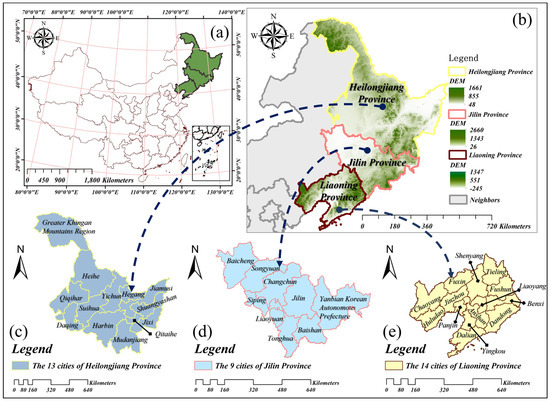
Figure 1.
Study area of northeast China. Note: Part (a) shows the map of China. Part (b) displays the location and boundary of Northeast China with 90 m DEM data. Parts (c–e) represent the administrative boundary at city scale of Heilongjiang, Jilin, and Liaoning Province, respectively. All geographic data were collected from the Geospatial Data Cloud: http://www.gscloud.cn (accessed on 25 June 2024).
The region primarily experiences a temperate monsoon climate. Due to its high latitude, Northeast China has distinct seasons, with long and cold winters in some areas. Geographically, it is characterized by plains and mountains rich in natural resources. Significant ecological barriers, such as the Greater and Lesser Khingan Mountains and Changbai Mountain, are located here, along with numerous wetlands and forest reserves such as the Zhalong Nature Reserve, Mao’er Mountain National Experimental Forest Farm, and Liangshui National Nature Reserve. This exceptional natural ecology provides a habitat for many wildlife species, including the Siberian tiger. Moreover, the fertile “black soil” in Northeast China makes it a leading region for producing crops such as corn and soybeans. The unique climate and natural resources of Northeast China significantly influence its population distribution, economy, and industrial development. Many of China’s military and automobile manufacturing enterprises are concentrated in this region, earning it the title of the “industrial cradle” of early China. During the 1950s and 1960s, it was China’s leading industrial area, with high levels of industrialization [40]. However, since the late 1970s to early 1980s, challenges such as resource depletion, the decline of traditional heavy industries, insufficient urban development momentum, and harsh climatic conditions have led to a sustained economic decline in Northeast China. These issues have also caused significant population loss and severe aging problems, particularly during the economic transition period, when many young workers migrated elsewhere, exacerbating the demographic imbalance. The recent census revealed that the aging population in Northeast China is among the highest in the country, reflecting the region’s long-standing socioeconomic challenges.
2.2. Study Data
In this paper, we employed three types of datasets to quantitatively estimate the estimation at the city scale, spatiotemporal evolution, and economic Tapio decoupling analysis of energy carbon emissions in northeast China.
2.2.1. Remote Sensing Data
Nighttime Light Data (NTL Data): In this study, we utilized two types of nighttime light data from different satellites: DMSP-OLS data and NPP-VIIRS data [46,47]. The DMSP-OLS data covers the period from 1992 to 2013, while the NPP-VIIRS data spans from 2012 to the present, monitored by the VIIRS instrument on the Suomi NPP satellite [26,48,49]. We selected DMSP-OLS data from 2005 to 2013 and NPP-VIIRS data from 2012 to 2019 for Northeast China at both provincial and city scales to estimate energy carbon emissions during the period from 2005 to 2019. The DN value (Digital Number) in DMSP-OLS data typically ranges from 0 to 63 [38], while in NPP-VIIRS data it does not have a fixed upper limit. It represents the light intensity of each pixel and is used to reflect urbanization levels and economic activity density. By analyzing changes in DN values, researchers can monitor urban expansion and energy consumption trends.
2.2.2. Statistical Data
Energy Consumption Data: The energy consumption data is sourced from the China Energy Statistical Yearbook (2006–2020). We have selected eight major types of energy: raw coal, coke, crude oil, gasoline, kerosene, diesel, fuel oil, and natural gas. Specifically, we use terminal energy consumption data from 2005 to 2019. Natural gas is measured in 100 million cubic meters, while the other energy types are measured in 10,000 tons.
Economic Data: We have selected GDP data from 2005 to 2019 for 36 cities in northeastern China. This data is obtained from several sources, including the Heilongjiang Statistical Yearbook (2006–2020), the Jilin Statistical Yearbook (2006–2020), the Liaoning Statistical Yearbook (2006–2020), the China City Statistical Yearbook (2006–2020), the Yanbian Korean Autonomous Prefecture Statistical Yearbook, and statistical bulletins from various prefectures and cities.
2.2.3. Emission Conversion Factors Data
The emission conversion factors mainly refer to the standard coal conversion factor and the carbon emission factor (Table 1). These data are sourced from the Intergovernmental Panel on Climate Change (IPCC) [41]. For natural gas, the standard coal conversion factor is 1.33 kg of standard coal per cubic meter (kg standard coal/m3).

Table 1.
Emission Factors and Conversion Data.
2.3. Methods
This section details the methods we employed, including statistical energy consumption at provincial scale, the estimation of energy carbon emissions using NTL data with the application of scaling, spatial autocorrelations, the calculation of SDE parameters and SLOPE values, and Tapio decoupling analysis. The research flow chart for our study is presented in Figure 2.
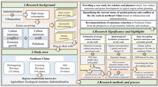
Figure 2.
Research Flow Chart.
2.3.1. Energy Carbon Emissions at the Provincial Scale
For the calculation of energy carbon emissions at the provincial scale, we follow the IPCC inventory method [32,50]. The statistical accounting of energy carbon emissions is based on energy consumption and carbon emission factors from the IPCC (Table 1), as shown in Formula (1). Those calculations will be utilized in estimating energy carbon emissions at city scale with scaling and NTL data. Throughout the entire analysis, the emissions were standardized by converting them to CO2 equivalents, represented as “CO2e”. Subsequent city-scale simulations were conducted using these standardized results.
In Formula (1), represents the energy carbon emissions (converted to equivalent) in year , represents the carbon emission factor for each energy type as provided by the IPCC, and represents the consumption of energy consumption type (converted to standard coal (ten thousand tons)). The numbers 44 and 12 represent the molecular weights of carbon and oxygen in , respectively.
2.3.2. Estimation of Energy Carbon Emissions at the City Scale: Scaling and NTL Data
NTL data, characterized by its high resolution and close correlation with urban development levels, population, and economy, is widely used in multi-scale simulations in areas such as ecology, urban activity, economy, population, and carbon emissions studies, promoting research on urban human-land relationships [7,8,9,10]. Traditional statistical accounting methods often suffer from limitations in manpower, resources, and data granularity, leading to data lack at smaller scales. To address this issue, we introduce the concept of scaling, which involves building relationships at a larger scale and then scaling these relationships to address smaller-scale issues within the same region. Specifically, the advantages of using NTL data in scaling include: (1) High spatial resolution: Ensures that data’s spatial details and features change minimally when scaling from provincial to city scale. (2) Data stability: Its spatial distribution is consistent across scales, making provincial-scale equations applicable at the city scale.
Based on these principles, we combine NTL data with the results of energy carbon emissions from the three northeastern provinces using the method proposed in Section 2.3.1 to estimate the energy carbon emissions from 2005 to 2019 at the city scale for 36 cities in northeast China. The steps are as follows: firstly, conversion and organization of two types of NTL data. Secondly, establishing the relationship between provincial scale energy carbon emissions and NTL data. Finally, scaling this relationship to estimate energy carbon emissions at the city scale.
- (1)
- Conversion and organization of two types of NTL data
Since the entire study period comprises two types of NTL data, i.e., DMSP-OLS (2005–2013) and NPP-VIIRS (2012–2019), it is necessary to convert and organize these datasets. Specifically, the NPP-VIIRS data from 2012 and 2013 (independent variable X) are used to establish a relationship with the DMSP-OLS data from the same years (dependent variable Y), since these years contain overlapping data for both datasets. Using this established relationship, all NPP-VIIRS data are converted to DMSP-OLS data [44], resulting in a complete DMSP-OLS dataset from 2005 to 2019, which is then used in subsequent steps [41].
In our study, we use linear, linear with intercept, and higher-order polynomial models up to cubic to fit the relationship between NPP-VIIRS data (independent variable) and DMSP-OLS data (dependent variable) for 2012 and 2013 [35,41,44]. To enhance accuracy, this step is performed separately for NTL data at both the provincial and city scales. Finally, using Eviews 7.2, the best-fitting results at both the provincial and city scales were obtained from the linear model with intercept, as shown in Formulas (2) and (3), respectively.
At a 95% confidence level, all parameters in both Formula (2) and (3) passed the Student’s t-test, with values of 0.9838 and 0.9090, respectively, and adjusted values of 0.9798 and 0.9077, respectively. The adjusted accounts for the number of predictors in the model, offering a more accurate measure of model fit by correcting the potential overestimation seen with the unadjusted , particularly in models with multiple predictors.
Specifically, represents the NPP-VIIRS data at the provincial scale from 2012 to 2013, while represents the DMSP-OLS data at the provincial scale from 2012 to 2013. and represent the data at the city scale.
Additionally, since 2012 and 2013 are the only years for which data are available in both DMSP-OLS and NPP-VIIRS, we used these years to establish the data conversion relationship. Utilizing Eviews 7.2, we assessed the representativeness of the 2012 and 2013 NPP-VIIRS data for other years using a simple linear function (Table 2). We then evaluated the correlation between the 2012 and 2013 NPP-VIIRS data and data from other years to determine their representativeness within the entire dataset. The results indicate that the NPP-VIIRS data from 2012 and 2013 are highly representative of the data from 2014 to 2019. Specifically, all parameters passed the Student’s t-test with a 95% confidence level, with all values of exceeding 0.95.
Table 2.
Representativeness Measurement Results of NPP-VIIRS Data: Comparing 2012, 2013, and 2014–2019.
- (2)
- Establishing the fitting relationship between provincial-scale emissions and NTL data
In this step, we use the converted and organized DMSP-OLS data from 2005 to 2019, along with the provincial-scale energy carbon emissions calculated in Section 2.3.1, to establish the fitting relationship between provincial-scale emissions and NTL data. Specifically, we tested various functions, including linear, linear with intercept, and up to cubic models. Ultimately, only the cubic function with intercept passed the significance test and demonstrated a strong ability to represent the relationship in the data. Using Eviews 7.2, we selected the cubic function with intercept for this relationship (Formula (4)). Based on Formula (4), the results are shown in Table 3, and the statistical test results of the model are presented in Table 4.
where represents the total DN values of NTL data [35] at the provincial scale, and represents the energy carbon emissions data at the provincial scale.
Table 3.
Fitting Relationship Between Provincial-Scale Energy Carbon Emissions and NTL Data.
Table 4.
Statistical Test Results of Model Parameters.
With significance levels set at 0.1 and 0.05, all parameters performed well in both the Student’s t-tests and Fisher’s F-tests. Additionally, the models’ values were as follows: Heilongjiang Province: 0.8135, Jilin Province: 0.7067, and Liaoning Province: 0.7653, demonstrating strong model fit and satisfactory explanatory power (Table 4).
- (3)
- Estimating energy carbon emissions at the city-scale based on scaling
In this step, our goal is to estimate city-scale energy carbon emissions using the processed city-scale nighttime light (NTL) data along with the concept of scaling. Based on the results from Table 3, we directly use the city-scale NTL data to estimate the energy carbon emissions at the city scale. However, the directly estimated results included the influence of nighttime lights, not the true estimation. To address this, we refer to the studies by Wu N et al. (2019) and GUAN Wei et al. (2022), using a grid correction factor. This correction factor helps make the energy carbon emissions for each grid more accurate in representing the true city-scale energy carbon emissions [35,41]. The whole process is represented in Formulas (5) and (6).
In Formulas (5) and (6), represents the grid correction factor. represents the true city-scale energy carbon emissions after correction in year n. represents the estimations of the energy carbon emissions, which include the influence of nighttime lights, obtained by applying the relationship in Table 3 for year n. and represent parameters from the grid perspective, i.e., the values in grid .
2.3.3. Spatiotemporal Evolution of Energy Carbon Emissions
We analyze the spatiotemporal evolution of energy carbon emissions by combining spatial statistics with geographic information systems, focusing on both spatial autocorrelation and spatial dynamic changes.
- (1)
- From the perspective of spatial autocorrelation: Moran’s I and Local Moran’s I
Spatial autocorrelation is a key concept in the first law of geography and is widely applied in both global and local spatial analysis. Global spatial autocorrelation is described by calculating Moran’s I (Formula (7)), which characterizes the overall spatial association of a variable across different spatial locations [6,9,44]. In contrast, local spatial autocorrelation is revealed by calculating Local Moran’s I (Formula (8)) [31,41,44], which identifies the spatial association and clustering characteristics of carbon emissions between local units and their neighboring units [45,51].
The global Moran’s I value ranges from −1 to 1. A positive value (0 to 1) indicates positive spatial autocorrelation, where similar attribute values are clustered together. Conversely, a negative value (−1 to 0) indicates negative spatial autocorrelation, where dissimilar attribute values are clustered together. Values closer to −1 or 1 signify stronger global spatial autocorrelation, while values near 0 indicate a random distribution with no spatial autocorrelation.
Local spatial autocorrelation is measured by Local Indicators of Spatial Association (LISA). When the Local Moran’s I is significant and positive, it indicates local positive spatial autocorrelation, represented by “High-High (H-H)” and “Low-Low (L-L)” clusters. H-H clusters signify that high values are surrounded by high values, while L-L clusters indicate that low values are surrounded by low values. On the other hand, a significant and negative Local Moran’s I indicate local negative spatial autocorrelation, represented by “High-Low (H-L)” and “Low-High (L-H)” outliers [52]. H-L outliers indicate a high value surrounded by low values, and L-H outliers indicate a low value surrounded by high values, both of which are anomalies compared to their surroundings.
In Formulas (7) and (8), represents the number of administrative units, which is 36 in this study. , represent the energy carbon emissions of city units , , respectively. represent the average energy carbon emissions of the 36 cities, and is the spatial weight matrix between neighboring city units , .
- (2)
- From the perspective of spatial dynamic changes
For the analysis of spatial dynamic changes, we selected the SDE parameters and SLOPE values.
Firstly, SDE parameters are one of the typical methods for analyzing spatial characteristics, including directionality, centroid shift, and overall spatial morphology. In this study, we characterized the SDE parameters for the energy carbon emissions and per capita energy carbon emissions at the city scale. By comparing different years, we interpreted the spatially dynamic changes in energy carbon emissions [42]. The formulas for calculating the SDE parameters are expressed as follows, from Formulas (9)–(12) [45,51,52]:
Here, and represent the horizontal and vertical coordinates of the standard deviation ellipse’s center point, respectively, which is typically the centroid of the study area; represents the energy carbon emissions values of the 36 cities in northeast China; and represent the lengths of the major and minor axes of the standard deviation ellipse, respectively, reflecting the spatial distribution characteristics of the data; represents the weight of regional emissions; and indicates the orientation angle of the standard deviation ellipse, representing the main direction of data distribution.
Secondly, we utilized the calculation of SLOPE values to classify the growth types of energy carbon emissions from 2005 to 2019. The classification standards are shown in Table 5. The calculation for SLOPE is expressed in Formula (13) [32,35].
Table 5.
Classification Standards for Growth Types in Energy Carbon Emissions.
In Formula (13), represents the total number of years in the study, which is 15 in this research, represents the year of carbon emissions measurement, ranging from 1 to 15 for the years 2005 to 2019, and represents the energy carbon emissions for the year .
2.3.4. Tapio Decoupling Analysis of Energy Carbon Emissions
Tapio decoupling, originally a concept from physics, refers to the situation where multiple variables are no longer interdependent [5], meaning that economic growth can occur without a corresponding increase in environmental pressure. This concept is now widely used for the quantitative assessment of the relationship between environmental pressure and economic development [6,53,54,55]. In this study, we employ the Tapio decoupling index, proposed by Tapio in 2005 [54], to analyze the relative changes in energy carbon emissions and GDP at the city scale in Northeast China. The formula for calculating the decoupling index and the decoupling types and their characteristics according to the Tapio decoupling index are shown in Formula (14) and Table 6, respectively.
Table 6.
Decoupling Types and Their Characteristics According to the Tapio Decoupling Index.
In Formula (14), the numerator represents the growth rate of carbon emissions, while the denominator can be understood as the GDP growth rate. represents the baseline energy carbon emissions.
3. Results
In this section, we present the results as follows: first, the statistical results at the provincial scale and the spatial patterns of the estimation results at the city scale; second, the spatial evolution, including spatial autocorrelation and spatial dynamic changes assessed by SDE and SLOPE values; finally, the conflicts between economic development and environmental pressure, quantified by the Tapio Decoupling Index.
3.1. Results of Energy Carbon Emissions at the City Scale in Northeast China
3.1.1. Statistical Results of Energy Carbon Emissions in Heilongjiang, Jilin, and Liaoning Provinces
Based on Formula (1), the energy carbon emissions for the three northeastern provinces of China were statistically calculated by R studio 4.3.2, as shown in Figure 3.
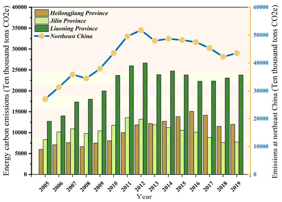
Figure 3.
Descriptive Statistical Analysis of Energy Carbon Emissions in Heilongjiang Province, Jilin Province, Liaoning Province, and Northeast China, 2005–2019.
Firstly, from 2005 to 2019, it is evident that Liaoning Province had significantly higher energy carbon emissions, with a minimum of 12,722 and a maximum of 26,672 ten thousand tons CO2e, compared to Heilongjiang Province, which had emissions between a minimum of 6000 and a maximum of 14,167 ten thousand tons CO2e, and Jilin Province, with a minimum of 7630 and a maximum of 13,579 ten thousand tons CO2e. Before 2013, the emission levels ranked as follows: Liaoning Province > Jilin Province > Heilongjiang Province. After 2013, Heilongjiang Province’s emissions surpassed those of Jilin Province, showing a slight upward trend. Liaoning Province’s emissions fluctuated mildly after 2013, while Jilin Province’s emissions continued to decline.
Secondly, regarding the overall energy carbon emissions of the three northeastern provinces, the total emissions had a minimum value of 27,071 and a maximum value of 51,770 ten thousand tons CO2e. The fluctuations can be divided into several periods: from 2005 to 2007, emissions increased during the first growth period, rising from 27,071 to 35,871 ten thousand tons CO2e; from 2007 to 2008, the first decline period occurred, with emissions decreasing from 35,871 to 34,471 ten thousand tons CO2e; from 2008 to 2012, emissions increased during the second growth period, rising from 34,471 to a peak of 51,770 ten thousand tons CO2e in 2012; from 2012 to 2013 and from 2013 to 2018, emissions decreased during the second and third decline periods, falling from 51,770 to 47,947 ten thousand tons CO2e, and then from 48,713 to 42,224 ten thousand tons CO2e, respectively, with the latter period showing a relatively stable decline; finally, from 2018 to 2019, emissions slightly increased, rising from 42,224 to 43,538 ten thousand tons CO2e.
3.1.2. Spatial Patterns of Energy Carbon Emissions in 36 Cities in Northeast China
Based on the natural breaking method, the emissions are classified into five categories, ranked from lowest to highest: “Low Emission”, “Moderately Low Emission”, “Medium Emission”, “Moderately High Emission”, and “High Emission”. Utilized ArcGIS 10.8, we selected data from the years 2005, 2010, 2015, and 2019 for analysis to easily observe their spatial distributions and dynamic changes (Figure 4). Combining the quantity and type patterns of carbon emissions, an in-depth discussion on the spatial patterns of 36 cities in northeast China is as follows:
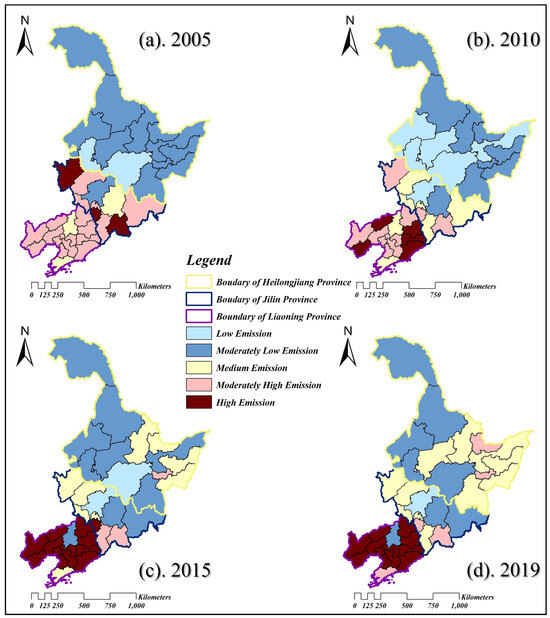
Figure 4.
Spatial Distribution of Energy Carbon Emissions in 36 Cities in Northeast China for the Years 2005 (a), 2010 (b), 2015 (c), and 2019 (d).
(1) Heilongjiang Province: Heilongjiang Province overall exhibits a trend where the western region maintains a consistent low-emission pattern, while the eastern region shows significant changes with gradually increasing emissions. Specifically, comparing 2005 and 2010, the “low emission” category expanded from Harbin and Daqing to include Qiqihar and Jiamusi. Other cities maintained a “moderately low emission” status during this period, with low carbon emission pressure. Comparing 2010 and 2015, the emission pattern changed significantly. Except for Harbin, areas with a “low emission” status in 2010 evolved to “moderately low emission” in 2015. Additionally, Yichun, Hegang, Shuangyashan, and Jixi transitioned from “moderately low emission” to “medium emission”, while Qitaihe evolved to “moderately high emission”. By 2019, the pattern changed less significantly than in 2015. Changes were observed only in Harbin, which shifted to “moderately low emission”, Mudanjiang, Suihua, and Jiamusi, which changed to “medium emission”, and Hegang, which became the second city in Heilongjiang with a “moderately high emission” status. The emission patterns of other cities remained unchanged.
(2) Jilin Province: Jilin Province overall exhibits a diverse pattern of emission types, with a trend towards lower carbon emission pressure. Specifically, in 2005, the pattern was disorganized, with a high proportion of “moderately high emissions”. By 2010, the patterns in nine cities shifted towards lower emission pressure, with Changchun and Jilin showing “low emissions”, Songyuan, Siping, Tonghua, and Yanbian evolving to “medium emissions”, and the other cities showing “moderately high emissions”. The “high emission” type had disappeared by this year. In 2015, the trend towards lower carbon emission pressure continued in most cities of Jilin Province. By 2019, there were minimal changes in the pattern, with only Liaoyuan and Tonghua showing positive changes in their carbon emission types, while the emission patterns in other cities remained unchanged.
(3) Liaoning Province: In 2005, among the 14 cities in Liaoning Province, except for Shenyang and Dalian, which were classified as “medium emissions”, all other cities were categorized as “moderately high emissions”, indicating a uniform pattern. By 2010, only Fuxin, Huludao, Fushun, Benxi, and Dandong changed to “high emissions”. From 2010 to 2015, most cities evolved into “high emissions”, with only Shenyang changing to “moderately low emissions”. This high carbon emission pressure pattern continued until 2019. Comparing 2005, 2010, 2015, and 2019, the overall trend in Liaoning Province was clear, with the level of emissions gradually increasing.
3.2. Spatiotemporal Evolution of Energy Carbon Emissions at the City Scale in Northeast China
3.2.1. Spatial Autocorrelation of Energy Carbon Emissions at the City Scale
Based on ArcGIS 10.8, we first calculated the global Moran’s I index for energy carbon emissions in Northeast China (Table 7). According to Table 7, the Z-scores of the global spatial autocorrelation Moran’s I for energy carbon emissions in 2005, 2010, 2015, and 2019 are all greater than 1.96, with p-values of 0.000 (p < 0.05). This indicates a statistically significant and positive spatial autocorrelation at the 95% confidence level, reflecting a significant degree of global spatial clustering of energy carbon emissions at the city scale. However, the degree of positive spatial autocorrelation in 2015 and 2019 is weaker compared to 2005 and 2010, based on the values of the global Moran’s I index.
Table 7.
Global Spatial Autocorrelation Moran’s I Calculation Results.
Secondly, based on Section 2.3.2, we can assess the degree of local Moran’s I. Specifically, we analyze the clustering between local units and their neighboring units using the LISA analysis (Figure 5). The details of the results are as follows:
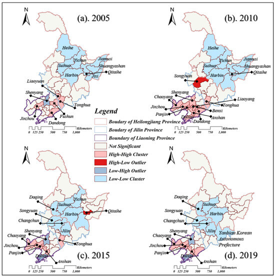
Figure 5.
Spatial Distribution of Local Moran’s I Calculated Using LISA for the Years 2005 (a), 2010 (b), 2015 (c), and 2019 (d).
Among the 36 cities in Northeast China observed in 2005, 2010, 2015, and 2019, areas with significant local spatial autocorrelation are mainly concentrated in Heilongjiang and Liaoning provinces. Specifically, the number of positive local spatial autocorrelations is higher than that of negative local spatial autocorrelations, and the spatial distribution patterns of positive correlations are relatively regular. The L-L clusters are mainly distributed in the central regions of Heilongjiang and Jilin provinces and the upper-central part of Northeast China, while the H-H clusters are primarily located in Liaoning province and a few border cities between Liaoning and Jilin provinces. In contrast, the number of cities with negative local spatial autocorrelations is smaller, primarily consisting of L-H outliers. The L-H outliers have only appeared in Liaoning province, while the H-L outliers have only appeared in Heilongjiang and Jilin provinces.
Comparing the LISA patterns across the four years reveals two distinct periods: 2005–2010 and 2015–2019. Firstly, in Heilongjiang province, a large number of L-L clusters were observed in 2005 and 2010. By 2015, these clusters spread to Jilin province, and an H-L outlier appeared in Heilongjiang. By 2019, the H-L outlier disappeared, and the number of L-L clusters decreased. In Jilin province, the LISA patterns were relatively simple in 2005 and 2010, with only a few significant clusters. In 2015, the number of significant clusters increased, showing a mix of L-L and H-H clusters, but by 2019, the clusters became more uniform, with only L-L clusters. Lastly, in Liaoning province, the clustering types were relatively uniform. Both H-H clusters and L-H outliers were present in 2005, 2015, and 2019, while in 2010, all significant clusters were H-H clusters.
3.2.2. Spatial Dynamic Changes of Energy Carbon Emissions
Firstly, as shown in Figure 6, using ArcGIS 10.8, the spatial distribution of the SDE for energy carbon emissions across 36 cities in Northeast China is as follows:
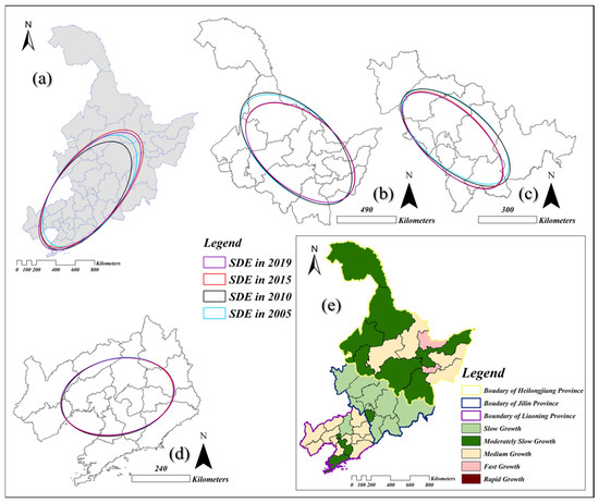
Figure 6.
Spatial Distribution of SDE and SLOPE Value in Northeast China. Note: Figure 6 presents general information on SDE and SLOPE values in Northeast China. (a) The dynamic change in SDE for Northeast China as a whole for the years 2005, 2010, 2015, and 2019. (b–d) The dynamic changes in SDE for Heilongjiang Province, Jilin Province, and Liaoning Province for the years 2005, 2010, 2015, and 2019, respectively. (e) The dynamic change in SLOPE values from 2005 to 2019 for Northeast China as a whole.
(1) From the perspective of dynamic changes in the energy carbon emission center and the range of changes in energy carbon emissions as indicated by the SDE, the following observations can be made. Specifically, as illustrated in Figure 6a, ranking the years based on the range of energy carbon emissions from largest to smallest is 2015, 2019, 2005, and 2010. The changes in the range of energy carbon emissions are more significant than those in the emission center. Additionally, the evolution pattern can be summarized as follows: from 2005 to 2010, the emission center clearly shifted towards the southwest, with the range significantly decreasing and increasingly covering Jilin and Liaoning provinces. From 2010 to 2015, the SDE indicated a clear shift in the center towards the northeast and a considerable expansion in the range. Finally, the changes in 2019 were minimal overall, with only slight changes in both the range of energy carbon emissions compared to 2015 and the center, which shifted slightly towards the southwest.
(2) From the perspective of each province, as shown in Figure 6b–d, the performance of the SDE in Heilongjiang province over the four years can be summarized by grouping the years based on similar patterns. Specifically, the years 2005 and 2010 form one group with similar SDE patterns, while 2015 and 2019 form another group. The emission ranges in the 2005 and 2010 group are significantly larger than those in the 2015 and 2019 group. Additionally, regarding the emission center, the directions in all four years are consistent, arranged from northwest to southeast. The spatial pattern of the SDE in Jilin province over the four years is similar to that in Heilongjiang province. Across the four years, the main change in energy carbon emissions was in the center, with minimal changes in range. Specifically, the center shifted from the northeast to the southwest in 2015 and 2019 compared to 2005 and 2010. Liaoning province showed the smallest changes among the provinces in Northeast China. The SDE parameters for energy carbon emissions in Liaoning province generally show a direction from southwest to northeast, with a relatively broad range and a centrally located emission center.
Secondly, to further analyze the growth trends of energy carbon emissions at the city scale in Northeast China from 2005 to 2019, we conducted an analysis based on the SLOPE classification standard and visualized the results using ArcGIS 10.8 (Figure 6e). Based on Table 5, we classified the growth types into five categories based on SLOPE values: Slow Growth (SLOPE value less than 16.0); Moderately Slow Growth (SLOPE value ranging from 16.0 to 47.5); Medium Growth (SLOPE value ranging from 47.5 to 63.2); Fast Growth (SLOPE value ranging from 63.2 to 78.9); Rapid Growth (SLOPE value greater than 78.9).
Specifically, there were no cities classified as “Rapid Growth” in Northeast China. The growth types of “Slow Growth” and “Moderately Slow Growth” were the most common among the 36 cities. Specifically, Heilongjiang province included three types of energy carbon emissions growth: “Moderately Slow Growth”, “Medium Growth”, and “Fast Growth”. The type of “Fast Growth” only appeared in Hegang and Qitaihe, which belong to Heilongjiang province. Except for Yichun, Suihua, Shuangyashan, and Jixi, which belong to the “Medium Growth” type, and Hegang and Qitaihe being “Fast Growth”, the other cities in Heilongjiang showed “Moderately Slow Growth”.
Liaoning province also included three types: “Slow Growth”, “Moderately Slow Growth”, and “Medium Growth”. Liaoyuan is the only one among the nine cities showing “Moderately Slow Growth”, while the others belong to “Slow Growth”, indicating that Jilin province had the smallest carbon emission pressure based on the growth type among Northeast China. Jilin province only included two types of energy carbon emissions growth: “Slow Growth” and “Moderately Slow Growth”. Among the 14 cities in Liaoning province, only Shenyang showed “Slow Growth”, Anshan and Dalian showed “Moderately Slow Growth”, while the others exhibited “Medium Growth”.
3.3. Economic Tapio Decoupling Analysis of Energy Carbon Emissions at the City Scale in Northeast China
In this section, by combining the use of R Studio 4.3.2 and ArcGIS 10.8, we perform Tapio decoupling analysis for five periods: 2005–2007, 2008–2010, 2011–2013, 2014–2016, and 2017–2019. Comparing these periods allows us to observe changes in the relationship between carbon emissions and economic growth. Additionally, we detail the steps involved, including the preprocessing of GDP data and the calculations of the Tapio decoupling index.
3.3.1. Data Preprocessing of GDP
The GDP data we obtained for each year are nominal GDP. Due to differing economic conditions each year, these values are not directly comparable to the absolute value of the RMB changes. Consequently, we utilize the GDP Deflator (with the base year set to 100 in the statistical yearbooks) to convert nominal GDP to real GDP, making it truly comparable. The process is shown in Formula (15).
In Formulas (14) and (15), the part of the Tapio decoupling index that involves GDP data is a fraction. Since the GDP deflator shows relatively small variations across those different years and is located in the denominator, it can be approximately simplified when calculating these formulas in our research. Additionally, our primary aim is to explore the relationship between carbon emissions and the economy, relying on the numerical range of the Tapio decoupling index for the macro classification of decoupling states rather than focusing on the absolute values of the decoupling index. Therefore, the impact of the GDP deflator on the decoupling index can be ignored, and the process described in Formula (15) can be omitted. Given this approach, we have reasonably addressed the challenge of collecting GDP deflator data for 36 cities over 15 years. Consequently, in subsequent research, we will directly use nominal GDP data to calculate the decoupling index for the 36 cities in Northeast China.
3.3.2. Results of Tapio Decoupling Analysis of Energy Carbon Emissions
Utilized ArcGIS 10.8, we performed tapio decoupling analysis in five groups (Figure 7). Additionally, by combining the relationship between economic development and environmental protection with the meaning of each decoupling state, we provide the intuitive evaluations for each decoupling state based on the Tapio decoupling index (Table 6) as follows: Strong Decoupling is evaluated as “Best”, Weak Decoupling as “Good”, Recessive Decoupling as “Fair”, Strong Negative Decoupling as “Worst”, Weak Negative Decoupling as “Poor”, Expansive Negative Decoupling as “Bad”, Expansive Coupling as “Average”, and Recessive Coupling as “Below Average”. These evaluations provide a clear understanding of how each decoupling state reflects the balance between economic growth and environmental impact.
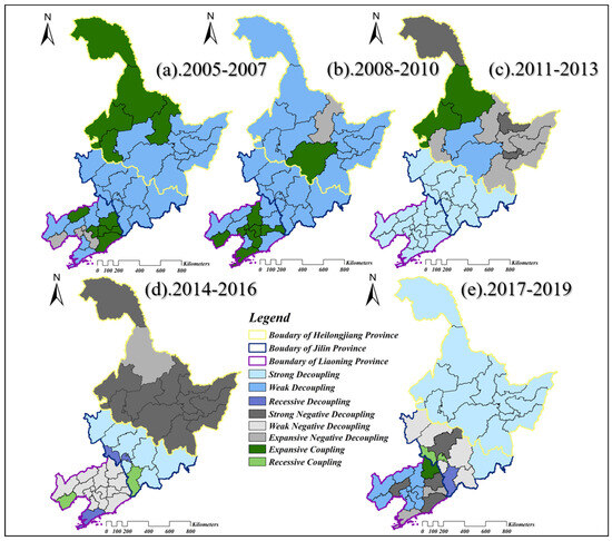
Figure 7.
Spatial Distribution of Tapio Decoupling Analysis in Northeast China, grouped by years 2005–2007 (a), 2008–2010 (b), 2011–2013 (c), 2014–2016 (d), and 2017–2019 (e).
- (1)
- Tapio Decoupling Analysis of 36 Cities in Northeast China, grouped by years from 2005 to 2007.
In Figure 7a, the simplified performance of the Tapio decoupling index for 36 cities in Northeast China from 2005 to 2007 is shown, with only three decoupling states: weak decoupling, expansive coupling, and expansive negative decoupling. Specifically, all nine cities in Jilin Province were in the weak decoupling state (“good”). Heilongjiang Province exhibited two types of decoupling states: expansive coupling (“average”), primarily distributed in the northwest of Heilongjiang Province, including Heihe, Yichun, Qiqihar, and Daqing, and weak decoupling (“good”) in other cities. Liaoning Province had the most diverse decoupling states with four types. Among them, Huludao, Panjin, and Anshan, where economic growth is slow and carbon emissions have significantly increased, showing the status of expansive negative decoupling, evaluated as “bad”.
- (2)
- Tapio Decoupling Analysis of 36 Cities in Northeast China, grouped by years from 2008 to 2010.
In this group, three decoupling states were presented. The overall pattern of the decoupling relationships was relatively simple. Apart from the nine cities in Jilin Province that remained in the same decoupling state (weak decoupling evaluated as “good”), there were changes in the decoupling states of Heilongjiang Province and Liaoning Province compared to the 2005 to 2007 grouping. In Heilongjiang Province, except for Yichun, which showed expansive negative decoupling (“bad”), and Harbin, which showed expansive coupling (“average”), other cities experienced two kinds of changes: one group changed from expansive coupling to weak decoupling (“good”), while the others maintained weak decoupling. The changes in the decoupling states in Liaoning Province were significant. For instance, Huludao, Panjin, and Anshan changed from expansive negative decoupling (“bad”) to expansive coupling (“average”). The rank of the degree of change in decoupling states, from most to least, is Liaoning Province, Heilongjiang Province, and Jilin Province.
- (3)
- Tapio Decoupling Analysis of 36 Cities in Northeast China, grouped by years from 2011 to 2013
This group exhibited a diversity of Tapio decoupling states, with the addition of strong decoupling and strong negative decoupling, resulting in a total of five decoupling states in Northeast China. Among them, strong decoupling was the most common, while weak decoupling and expansive coupling were the least common. Additionally, comparing with the previous group, the patterns of decoupling states in Liaoning Province and Jilin Province were relatively consistent, both showing the strong decoupling state in each city. In contrast, Heilongjiang Province showed a more complex and diverse pattern of decoupling states, with four decoupling states exhibited in its 13 cities. Specifically, from northwest to southeast, the Greater Khingan Range (strong negative decoupling, evaluated as worst), Heihe (strong negative decoupling, evaluated as worst), Qiqihar (expansive coupling, evaluated as average), Yichun (expansive negative decoupling, evaluated as bad), Daqing (expansive negative decoupling, evaluated as bad), Suihua (weak decoupling, evaluated as good), Hegang (strong negative decoupling, evaluated as worst), Jiamusi (expansive negative decoupling, evaluated as bad), Harbin (weak decoupling, evaluated as good), Qitaihe (strong negative decoupling, evaluated as worst), Shuangyashan (expansive negative decoupling, evaluated as bad), Jixi (expansive negative decoupling, evaluated as bad), and Mudanjiang (expansive negative decoupling, evaluated as bad).
- (4)
- Tapio Decoupling Analysis of 36 Cities in Northeast China, grouped by years from 2014 to 2016
The increasing number of Tapio decoupling states was still occurring. In this group, there were six in 36 cities, with the addition of recessive coupling, weak negative decoupling, and recessive decoupling, while weak decoupling and expansive coupling were gone compared with previous groups. Specifically, in Jilin Province, there were changes in Siping and Tonghua to recessive decoupling (‘fair”) and recessive coupling (“below average”), respectively, while the other seven cities maintained strong decoupling (“best”). In this group, significant changes occurred in Liaoning Province, with changes in all 14 cities. For example, Huludao and Dalian changed to recessive coupling (“below average”) and recessive decoupling (“fair”), respectively, while the other 12 cities changed to weak negative decoupling (“poor”). In Heilongjiang Province, except for Heihe, which showed the Tapio decoupling state with expansive negative decoupling (“bad”), the other 12 cities were in strong negative decoupling (“worst”).
- (5)
- Tapio Decoupling Analysis of 36 Cities in Northeast China, grouped by years from 2017 to 2019
From 2017 to 2019, the number of Tapio decoupling states increased to eight, with the addition of strong negative decoupling and the reappearance of weak decoupling. Specifically, strong decoupling was the most common Tapio decoupling state, uniformly distributed across half of Northeast China. Expansive coupling, recessive coupling, and recessive decoupling each appeared only once in three different cities. Heilongjiang Province’s Tapio decoupling state performance was uniformly consistent, while Liaoning Province and Jilin Province exhibited more complex and diverse changes during this period. In Jilin Province, five Tapio decoupling states were observed: weak negative decoupling (“poor”), strong negative decoupling (“worst”), strong decoupling (“best”), recessive coupling (“below average”), and recessive decoupling (“fair”). Liaoning Province displayed four states: expansive negative decoupling (“bad”), expansive coupling (“average”), weak decoupling (“good”), and strong negative decoupling (“worst”). In summary, from 2017 to 2019, the evaluation of Tapio decoupling states in Northeast China showed excellent performance in Heilongjiang Province and Liaoning Province, while Jilin Province performed relatively poorly.
4. Discussion
The analysis of the results in Section 3 provides valuable insights into the quantitative and spatial characteristics of energy carbon emissions in Northeast China, a typical industrialized region. These insights help address the environmental, demographic, and economic challenges associated with rapid urbanization and can serve as a guide for policymakers in their decision-making processes [40]. This section focuses on interpreting the Results and offering recommendations to reduce energy carbon emissions in Northeast China, considering the perspectives of government, industry, and residents [39].
4.1. Result Analysis and Interpretation
4.1.1. Spatial Patterns of Energy-Related Carbon Emissions
From 2005 to 2019, energy carbon emissions in Northeast China exhibited significant spatial and temporal variations across different provinces and cities. Firstly, Liaoning Province consistently had significantly higher energy carbon emissions compared to Heilongjiang and Jilin Provinces. Liaoning’s emissions ranged from a minimum of 12,722 to a maximum of 26,672 ten thousand tons of CO2e during this period. This is closely related to the dominance of heavy industries in Liaoning’s economic structure, such as steel, machinery manufacturing, and energy-intensive industries, which make it the largest emitter among the three provinces. In contrast, Heilongjiang and Jilin had lower emission levels. Heilongjiang’s emissions ranged from 6000 to 14,167 ten thousand tons CO2e, while Jilin’s emissions fluctuated between 7630 and 13,579 ten thousand tons CO2e.
4.1.2. Spatiotemporal Evolution of Energy-Related Carbon Emissions: Spatial Autocorrelation of Emissions and Shifts in Emission Centers
A significant shift occurred after 2013, when Heilongjiang’s carbon emissions surpassed those of Jilin. This upward trend in Heilongjiang likely reflects structural changes in the province’s energy use, possibly linked to increased coal consumption or industrial expansion. Meanwhile, Jilin experienced a continuous decline in emissions after 2013, indicating that the province might have implemented effective measures to reduce carbon emissions and improve energy efficiency. These dynamics demonstrate different approaches taken by the three provinces in balancing energy consumption and economic development.
From a spatial perspective, the spatial autocorrelation analysis revealed clear regional clustering effects of carbon emissions. The global Moran’s I index was positive, indicating that high-emission areas are often located near other high-emission areas. Particularly in Liaoning and Heilongjiang, the local Moran’s I analysis identified significant clusters of high emissions, especially in industrialized cities such as Shenyang and Dalian in Liaoning. These cities not only drive economic growth but are also major sources of carbon emissions. In Heilongjiang, clustering around Harbin reflects the province’s industrial concentration and energy production patterns.
The SDE analysis further highlighted the spatiotemporal evolution of carbon emission centers. During the study period, the center of carbon emissions gradually shifted northwestward, with the most significant changes occurring in 2015. This shift likely reflects regional economic adjustments, such as the economic slowdown in some cities and changes in energy consumption patterns. The movement of the emission center also suggests varying progress in emission reduction and energy transition policies across different cities within the region.
4.1.3. Tapio Decoupling of Economic Growth and Carbon Emissions
The Tapio decoupling analysis provided critical insights into the relationship between economic growth and carbon emissions. The results show that Heilongjiang achieved “absolute decoupling”, meaning that while the economy grew, carbon emissions decreased, indicating significant progress in balancing economic and environmental sustainability. This could be attributed to the province’s adoption of cleaner energy sources and improvements in industrial efficiency. In contrast, Jilin exhibited weaker decoupling or even “re-coupling”, meaning that emissions did not decrease significantly despite economic growth. This suggests that Jilin may be facing challenges in restructuring its economy or implementing effective emission reduction measures. Liaoning presented a more complex case, with little change in the relationship between economic growth and carbon emissions, indicating that the province is struggling to reduce emissions, particularly given its reliance on high-emission industries.
4.2. Policy Recommendations
4.2.1. Recommendations from the Perspective of Government
Firstly, the government should actively implement policies to guide high-emission enterprises in energy conservation and emission reduction. Northeast China, primarily focused on industrial manufacturing, includes high-emission industries such as large-scale military industries in Heilongjiang Province and automobile manufacturing in Changchun. These enterprises are major sources of energy consumption and carbon emissions. The government should strictly control resource consumption, reduce unnecessary resource wastage, and achieve low-energy development. For high-emission enterprises, the government should establish and implement emission reduction tasks, encourage evaluations on carbon emissions reduction, and complete emission reduction tasks through carbon trading and other means, promoting the development and improvement of the carbon market.
Secondly, the government should promote technological innovation and the development of green resources to achieve pollution and carbon reduction. Enterprises, universities, and research institutions should be encouraged to innovate and optimize existing industrial technologies, improving the conversion and application rates of research outcomes. The rational development of existing green resources, such as forests, water, and land, should be explored for their potential in emission reduction and consumption substitution. Cross-departmental cooperation and research should be promoted to achieve sustainable development and utilization of resources. For urban emission regulation, the government should consider population and geographical location to develop targeted policies. Northeast China faces severe issues of population loss and aging, especially in sparsely populated areas of Heilongjiang Province. Policies should be implemented to coordinate resource flow and optimize the match between population and emissions. Additionally, the geographical diversity of Northeast China, with cities near the coast and borders, requires special attention. Managing the relationship between resources, trade, and emissions is essential to prevent carbon emission spillovers and cross-regional flows.
Thirdly, the government should also support green industries to lead “green-oriented” rural revitalization. Green industries, such as eco-tourism and forest therapy, are low-emission and low-energy industries that effectively balance emissions and economic development. Utilizing green resources can achieve rural revitalization, increase employment rates, and develop agricultural products, thereby enhancing regional economies. Developing forest carbon sinks and afforestation can improve the sustainability of resources and enhance carbon sink benefits.
Finally, the government should strengthen the construction of industry databases to support emission reduction-oriented academic research. Monitoring and managing data is the foundation for policy formulation. Industry databases should be established to conduct quantitative statistical accounting, providing a basis for decision-making. By improving databases, quantitative monitoring of carbon emissions can be strengthened, promoting academic research and supporting industrial green and low-carbon innovation.
4.2.2. Recommendations from the Perspective of Industry
Industries are a crucial part of the market, influencing supply and demand dynamics, and are a major source of carbon emissions. Industries should leverage collective strengths, focus on the green transformation of products and services, and contribute to the dual carbon goals. From the product manufacturing perspective, while ensuring profitability, industries should increase the use of new energy sources to replace traditional fossil fuels, achieving the goal of green product development. Examples include wind, hydro, and solar power generation, as well as the rising market share of new energy vehicles. In the service supply sector, green transformation should be the primary goal, with collective efforts focusing on sustainable use with a protection-first approach. Forestry enterprises such as Yichun Forest Industry Group maintain forest areas under strict logging bans. In the product processing sector, the green transformation of packaging materials has been widely adopted, as seen in the use of biodegradable packaging bags and eco-friendly materials in clothing products.
Additionally, industries should actively focus on emission reduction targets, committing to high-quality completion of these tasks and aligning closely with government policies. Appropriate methods such as carbon offset forestry and carbon trading should be selected. Enterprises should also act as hubs, providing platforms for the integration and development of technologies across different fields and leveraging cross-industry strengths for complementary advantages. Key practices include the integration of ecological resources with the tourism industry to form eco-tourism and the combination of forest resources with traditional health industries to create forest therapy. These green industries exhibit significant synergies between emission reductions and economic growth.
4.2.3. Recommendations from the Perspective of Residents
Firstly, residents should actively participate in the dissemination and investigation of pollution emissions and waste sorting. This involves engaging in educational and social research activities organized by communities, streets, and various departments. Residents should learn to identify emission sources, avoid excessive pollution, and apply these practices in daily life. By correctly sorting and processing waste, residents can significantly reduce the costs and efforts of waste reprocessing, directly lowering carbon emissions from a resource consumption perspective. Additionally, residents can provide key data for “behavioral” emission studies by participating in surveys and research on topics such as waste sorting willingness and commuting behavior. This type of social science research can offer valuable insights for green development, helping to adjust structures and patterns to achieve emission reductions from the residents’ perspective while raising awareness about sustainable strategies.
Secondly, as the main agents of consumption behavior, residents can be encouraged and nurtured towards green consumption through relevant government incentive policies. Ensuring support for green consumption across different age groups and promoting interactive activities to raise energy conservation and emission reduction awareness is crucial. For instance, pilot programs in public spaces, such as metro stations offering only electronic tickets during certain periods, can promote green commuting. Additionally, building a comprehensive commuting database can further support the development of low-carbon cities.
5. Conclusions
After conducting the whole process of estimation on energy carbon emissions at city scale by scaling and using NTL data, we obtained the results of spatial autocorrelation in global and local, dynamic changes, and the tapio decoupling analysis at city scale in northeast China. The conclusion of the spatiotemporal evolution and patterns of it are summarized as follows:
5.1. Conclusion of Spatial Patterns of Energy Carbon Emissions
The spatiotemporal evolution of energy carbon emissions in the 36 cities of Heilongjiang Province exhibits distinct patterns. The western regions show a single emission pattern with low emission levels, while the eastern regions display diverse patterns with steadily increasing emissions. Overall, Heilongjiang Province primarily exhibits low emissions, though there has been a slight trend toward increasing emissions in recent years. In Jilin Province, the types of energy carbon emissions are more varied and complex. The overall trend is positive, shifting from predominantly high emissions to gradually decreasing emission levels. Liaoning Province’s emission patterns are similar to those of Heilongjiang, characterized by a single, increasingly severe emission pattern. Starting with high emissions, the province has progressively moved towards even higher emission levels over time.
5.2. Conclusion of Spatiotemporal Evolution of Energy Carbon Emissions
Spatial Autocorrelation: From 2005 to 2019, the global spatial autocorrelation of energy carbon emissions in the northeastern provinces was significant and positive, with p-values consistently at 0.000, indicating notable spatial clustering. The correlation was weaker in 2015, 2016, and 2017 (Moran’ s I < 0.5) and stronger in 2010 and 2011 (Moran’ s I > 0.7). Locally, significant spatial autocorrelation was mainly in Heilongjiang and Liaoning. Positive autocorrelation was more prevalent and concentrated, with “L-L” clusters in central Heilongjiang and Jilin and “H-H” clusters in parts of Liaoning and Jilin. Negative correlations were less common, with “L-H” outliers in Liaoning and “H-L” outliers in Heilongjiang and Jilin.
SDE Parameters: The SDE analysis showed that emission ranges from 2005 to 2019 were most extensive in 2015 and smallest in 2010. Range variation exceeded centroid movement. In Heilongjiang, SDE parameters for 2005 and 2010 were similar, as were 2015 and 2019. The emission centroids moved consistently from northwest to southeast. In Jilin, centroids also aligned northwest to southeast, with minor range changes. Liaoning showed minimal change, with a broad range and central centroid from southwest to northeast.
SLOPE Value: No “rapid growth” in emissions was observed from 2005 to 2019. “Fast growth” occurred only in Hegang and Qitaihe. Predominant growth types were “slow” and “very slow”. Heilongjiang had the most diverse growth types, Liaoning had three, and Jilin was the most uniform with two types. Overall, emission growth rates were fastest in Heilongjiang, followed by Liaoning, and slowest in Jilin.
5.3. Conclusion of the Tapio Decoupling Relationship
In analyzing the decoupling state of the relationship between carbon emissions and the economy, this study evaluated the trends in economic development and carbon emissions. Heilongjiang Province is the only province among the three that successfully adjusted its decoupling status. Over the first four periods, its decoupling evaluation consistently declined, but from 2017 to 2019, it recovered and showed the best decoupling evaluation across the province. In contrast, Jilin Province’s decoupling quality gradually declined from an initially diverse pattern. The decline was not significant in the first four periods, but from 2017 to 2019, all cities except Yanbian Prefecture showed low decoupling evaluations. Liaoning Province’s decoupling evaluation remained relatively stable over the five periods, with no significant decline in quality, except for a period of low evaluation from 2014 to 2016.
Author Contributions
B.L.: Writing—original draft, Writing—review and editing, Visualization, Software, Methodology, Investigation, Formal analysis, Data curation, and Conceptualization. J.L.: Writing—review and editing, Funding acquisition, and Project administration, Resources. All authors have read and agreed to the published version of the manuscript.
Funding
This work was supported by the National Social Science Foundation of China (Grant No. 21BGL166) under the project titled “Analysis of the Balanced Matching between Greenhouse Gas Emission Control and Forest Carbon Sequestration and Policy Implications”.
Data Availability Statement
The data sets used in this study will be made available upon request.
Conflicts of Interest
The authors declare no conflicts of interest.
References
- Guan, X.; Wei, H.; Lu, S.; Dai, Q.; Su, H. Assessment on the urbanization strategy in China: Achievements, challenges and reflections. Habitat Int. 2018, 71, 97–109. [Google Scholar] [CrossRef]
- Dong, R.; Yan, F. Revealing Characteristics of the Spatial Structure of Megacities at Multiple Scales with Jobs-Housing Big Data: A Case Study of Tianjin, China. Land 2021, 10, 1144. [Google Scholar] [CrossRef]
- Shen, H.; Tao, S.; Chen, Y.; Ciais, P.; Güneralp, B.; Ru, M.; Zhong, Q.; Yun, X.; Zhu, X.; Huang, T.; et al. Urbanization-induced population migration has reduced ambient PM2.5 concentrations in China. Sci. Adv. 2017, 3, e1700300. [Google Scholar] [CrossRef] [PubMed]
- Johnson, M.T.J.; Munshi-South, J. Evolution of life in urban environments. Science 2017, 358, eaam8327. [Google Scholar] [CrossRef]
- Lai, W.; Hu, Q.; Zhou, Q. Decomposition analysis of PM2.5 emissions based on LMDI and Tapio decoupling model: Study of Hunan and Guangdong. Environ. Sci. Pollut. Res. 2021, 28, 43443–43458. [Google Scholar] [CrossRef]
- Ding, Y.; Zhang, M.; Chen, S.; Wang, W.; Nie, R. The environmental Kuznets curve for PM2.5 pollution in Beijing-Tianjin-Hebei region of China: A spatial panel data approach. J. Clean. Prod. 2019, 220, 984–994. [Google Scholar] [CrossRef]
- Murayama, Y.; Wang, R. Editorial: Special Issue on Geographical Analysis and Modeling of Urban Heat Island Formation. Remote Sens. 2023, 15, 4474. [Google Scholar] [CrossRef]
- Allen, M.R.; Frame, D.J.; Huntingford, C.; Jones, C.D.; Lowe, J.A.; Meinshausen, M.; Meinshausen, N. Warming caused by cumulative carbon emissions towards the trillionth tonne. Nature 2009, 458, 1163–1166. [Google Scholar] [CrossRef]
- Wang, X.; Cai, Y.; Liu, G.; Zhang, M.; Bai, Y.; Zhang, F. Carbon emission accounting and spatial distribution of industrial entities in Beijing—Combining nighttime light data and urban functional areas. Ecol. Inform. 2022, 70, 101759. [Google Scholar] [CrossRef]
- Liu, Y. Exploring the relationship between urbanization and energy consumption in China using ARDL (autoregressive distributed lag) and FDM (factor decomposition model). Energy 2009, 34, 1846–1854. [Google Scholar] [CrossRef]
- Hu, J.; Gui, S.; Zhang, W. Decoupling Analysis of China’s Product Sector Output and Its Embodied Carbon Emissions—An Empirical Study Based on Non-Competitive I-O and Tapio Decoupling Model. Sustainability 2017, 9, 815. [Google Scholar] [CrossRef]
- Zhang, C.; Lu, N.; Chen, Y. Decoupling Analysis of Economic Growth and Carbon Emissions from the Perspective of City Scale. IOP Conf. Ser. Earth Environ. Sci. 2019, 295, 052010. [Google Scholar] [CrossRef]
- Zhao, X.; Jiang, M.; Zhang, W. Decoupling between Economic Development and Carbon Emissions and Its Driving Factors: Evidence from China. Int. J. Environ. Res. Public Health 2022, 19, 2893. [Google Scholar] [CrossRef] [PubMed]
- Wei, Z.; Wei, K.; Liu, J. Decoupling relationship between carbon emissions and economic development and prediction of carbon emissions in Henan Province: Based on Tapio method and STIRPAT model. Environ. Sci. Pollut. Res. 2023, 30, 52679–52691. [Google Scholar] [CrossRef] [PubMed]
- Dong, Z.; Zhang, Z.; Zhang, F. Coupling coordination development of energy-economy-carbon emissions in China under the background of ‘double carbon’. PLoS ONE 2022, 17, e0277828. [Google Scholar] [CrossRef]
- Chen, M.; Zhao, S.; Wang, J. The Impact of the Digital Economy on Regional Carbon Emissions: Evidence from China. Sustainability 2023, 15, 14863. [Google Scholar] [CrossRef]
- Wang, Q.; Huang, J.; Zhou, H.; Sun, J.; Yao, M. Carbon Emission Inversion Model from Provincial to Municipal Scale Based on Nighttime Light Remote Sensing and Improved STIRPAT. Sustainability 2022, 14, 6813. [Google Scholar] [CrossRef]
- Li, Y.; Gao, H.; Sun, W. Analysis of the Decoupling Relationship between China’s Economy and the Indicators of the Power Industry from National and Provincial Aspects. Pol. J. Environ. Stud. 2020, 29, 4183–4198. [Google Scholar] [CrossRef]
- Geng, Y.; Fujita, T.; Chiu, A.; Dai, H.; Hao, H. Responding to the Paris Climate Agreement: Global climate change mitigation efforts. Front. Energy 2018, 12, 333–337. [Google Scholar] [CrossRef]
- Schleussner, C.-F.; Ganti, G.; Rogelj, J.; Gidden, M.J. An emission pathway classification reflecting the Paris Agreement climate objectives. Commun. Earth Environ. 2022, 3, 135. [Google Scholar] [CrossRef]
- Kuyper, J.; Schroeder, H.; Linnér, B.-O. The Evolution of the UNFCCC. Annu. Rev. Environ. Resour. 2018, 43, 343–368. [Google Scholar] [CrossRef]
- Lin, D.; Allan, A.; Cui, J. The impact of polycentric urban development on commuting behaviour in urban China: Evidence from four sub-centres of Beijing. Habitat Int. 2015, 50, 195–205. [Google Scholar] [CrossRef]
- Fang, C.; Wang, S.; Li, G. Changing urban forms and carbon dioxide emissions in China: A case study of 30 provincial capital cities. Appl. Energy 2015, 158, 519–531. [Google Scholar] [CrossRef]
- Wang, S.; Fang, C.; Guan, X.; Pang, B.; Urbanisation, H.M. Energy consumption, and carbon dioxide emissions in China: A panel data analysis of China’s provinces. Appl. Energy 2014, 136, 738–749. [Google Scholar] [CrossRef]
- Shi, K.; Chen, Y.; Yu, B.; Xu, T.; Chen, Z.; Liu, R.; Li, L.; Wu, J. Modeling spatiotemporal CO2 (carbon dioxide) emission dynamics in China from DMSP-OLS nighttime stable light data using panel data analysis. Appl. Energy 2016, 168, 523–533. [Google Scholar] [CrossRef]
- Zhao, M.; Zhou, Y.; Li, X.; Cao, W.; He, C.; Yu, B.; Li, X.; Elvidge, C.D.; Cheng, W.; Zhou, C. Applications of Satellite Remote Sensing of Nighttime Light Observations: Advances, Challenges, and Perspectives. Remote Sens. 2019, 11, 1971. [Google Scholar] [CrossRef]
- Liu, Z.; He, C.; Zhang, Q.; Huang, Q.; Yang, Y. Extracting the dynamics of urban expansion in China using DMSP-OLS nighttime light data from 1992 to 2008. Landsc. Urban Plan. 2012, 106, 62–72. [Google Scholar] [CrossRef]
- Liu, H.; Ma, L.; Xu, L. Estimating spatiotemporal dynamics of county-level fossil fuel consumption based on integrated nighttime light data. J. Clean. Prod. 2021, 278, 123427. [Google Scholar] [CrossRef]
- Shi, K.; Chen, Y.; Li, L.; Huang, C. Spatiotemporal variations of urban CO2 emissions in China—A multiscale perspective. Appl. Energy 2018, 211, 218–229. [Google Scholar] [CrossRef]
- Oda, T.; Maksyutov, S. A very high-resolution (1 km × 1 km) global fossil fuel CO2 emission inventory derived using a point source database and satellite observations of nighttime lights. Atmos. Chem. Phys. 2011, 11, 543–556. [Google Scholar] [CrossRef]
- Wang, S.; Liu, X. China’s city-level energy-related CO2 emissions: Spatiotemporal patterns and driving forces. Appl. Energy 2017, 200, 204–214. [Google Scholar] [CrossRef]
- Su, Y.; Chen, X.; Li, Y.; Liao, J.; Ye, Y.; Zhang, H.; Huang, N.; Kuang, Y. China׳s 19-year city-level carbon emissions of energy consumptions, driving forces and regionalized mitigation guidelines. Renew. Sustain. Energy Rev. 2014, 35, 231–243. [Google Scholar] [CrossRef]
- Ghosh, T.; Elvidge, C.D.; Sutton, P.C.; Baugh, K.E.; Ziskin, D.; Tuttle, B.T. Creating a Global Grid of Distributed Fossil Fuel CO2 Emissions from Nighttime Satellite Imagery. Energies 2010, 3, 1895–1913. [Google Scholar] [CrossRef]
- Zhao, J.; Chen, Y.; Ji, G.; Wang, Z. Residential carbon dioxide emissions at the urban scale for county-level cities in China: A comparative study of nighttime light data. J. Clean. Prod. 2018, 180, 198–209. [Google Scholar] [CrossRef]
- Wu, N.; Shen, L.; Zhong, S. Spatio-temporal pattern of carbon emissions based on nightlight data of Shanxi-Shaanxi-Inner Mongolia region of China. J. Geo-Inf. Sci. 2019, 21, 1040–1050. [Google Scholar] [CrossRef]
- Yunyan, L.; Qing, S.; Jian, D. Spatio-temporal Characteristics of Carbon Emission in Beijing-Tianjin-Hebei Urban Agglomeration Derived from Integrated DMSP-OLS and NPP-VIIRS Nighttime Light Data. J. Environ. Eng. Technol. 2023, 13, 447–454. [Google Scholar]
- Meng, L.; Graus, W.; Worrell, E.; Huang, B. Estimating CO2 (carbon dioxide) emissions at urban scales by DMSP/OLS (Defense Meteorological Satellite Program’s Operational Linescan System) nighttime light imagery: Methodological challenges and a case study for China. Energy 2014, 71, 468–478. [Google Scholar] [CrossRef]
- Xiao, H.; Ma, Z.; Mi, Z.; Kelsey, J.; Zheng, J.; Yin, W.; Yan, M. Spatio-temporal simulation of energy consumption in China’s provinces based on satellite night-time light data. Appl. Energy 2018, 231, 1070–1078. [Google Scholar] [CrossRef]
- Gao, Z.; Li, S.; Cao, X.; Li, Y. Carbon Emission Intensity Characteristics and Spatial Spillover Effects in Counties in Northeast China: Based on a Spatial Econometric Model. Land 2022, 11, 753. [Google Scholar] [CrossRef]
- Zhang, P. Revitalizing old industrial base of Northeast China: Process, policy and challenge. Chin. Geogr. Sci. 2008, 18, 109–118. [Google Scholar] [CrossRef]
- Wei, G.; Shumei, L.; Shuting, X. Multiscale Spatio-Temporal Characteristics of Carbon Emissions in Northeast China Based on DMSP/OLS Nighttime Light Data. Ecol. Econ. 2022, 38, 19–26. [Google Scholar]
- Di, Y.; Xu, Y.; Xiangli, W.; Yuanhe, C.; Jia, Z.; Dasha, F.; Chang, Z. Spatio-temporal evolution characteristics of carbon emissions from energy consumption and its driving mechanism in Northeast China. Acta Sci. Circumstantiae 2018, 38, 4554–4564. [Google Scholar] [CrossRef]
- Liu, X.; Duan, Z.; Shan, Y.; Duan, H.; Wang, S.; Song, J.; Wang, X. Low-carbon developments in Northeast China: Evidence from cities. Appl. Energy 2019, 236, 1019–1033. [Google Scholar] [CrossRef]
- Liu, X.; Duan, Z.; Shan, Y.; Duan, H.; Wang, S.; Song, J.; Wang, X. Multiscale Spatio-Temporal Characteristics of Carbon Emission of Energy Consumption in Yellow River Basin Based on the Nighttime Light Datasets. Econ. Geogr. 2020, 40, 12–21. [Google Scholar]
- Zhang, W.; Shi, P.; Huang, W. Research on Spatial and Temporal Pattern Evolution and Driving Factors of County Carbon Emissions in Underdeveloped Regions: Gansu Province of Western China as an Example. Sustainability 2022, 15, 291. [Google Scholar] [CrossRef]
- Zhang, X.; Wu, J.; Peng, J.; Cao, Q. The Uncertainty of Nighttime Light Data in Estimating Carbon Dioxide Emissions in China: A Comparison between DMSP-OLS and NPP-VIIRS. Remote Sens. 2017, 9, 797. [Google Scholar] [CrossRef]
- Sun, Y.; Zheng, S.; Wu, Y.; Schlink, U.; Singh, R.P. Spatiotemporal Variations of City-Level Carbon Emissions in China during 2000–2017 Using Nighttime Light Data. Remote Sens. 2020, 12, 2916. [Google Scholar] [CrossRef]
- Zhu, Y.; Xu, D.; Ali, S.H.; Ma, R.; Cheng, J. Can Nighttime Light Data Be Used to Estimate Electric Power Consumption? New Evidence from Causal-Effect Inference. Energies 2019, 12, 3154. [Google Scholar] [CrossRef]
- Zhang, H.; Yu, Q.; Liu, Y.; Jiang, J.; Chen, J.; Liu, R. The Spatio-Temporal Patterns of Regional Development in Shandong Province of China from 2012 to 2021 Based on Nighttime Light Remote Sensing. Sensors 2023, 23, 8728. [Google Scholar] [CrossRef]
- Sun, L.; Mao, X.; Feng, L.; Zhang, M.; Gui, X.; Wu, X. Investigating the Direct and Spillover Effects of Urbanization on Energy-Related Carbon Dioxide Emissions in China Using Nighttime Light Data. Remote Sens. 2023, 15, 4093. [Google Scholar] [CrossRef]
- Yuan, W.; Sun, H.; Chen, Y.; Xia, X. Spatio-Temporal Evolution and Spatial Heterogeneity of Influencing Factors of SO2 Emissions in Chinese Cities: Fresh Evidence from MGWR. Sustainability 2021, 13, 12059. [Google Scholar] [CrossRef]
- Yang, Z.; Sun, H.; Yuan, W.; Xia, X. The Spatial Pattern of the Prefecture-Level Carbon Emissions and Its Spatial Mismatch in China with the Level of Economic Development. Sustainability 2022, 14, 10209. [Google Scholar] [CrossRef]
- Wang, K.; Zhu, Y.; Zhang, J. Decoupling economic development from municipal solid waste generation in China’s cities: Assessment and prediction based on Tapio method and EKC models. Waste Manag. 2021, 133, 37–48. [Google Scholar] [CrossRef] [PubMed]
- Tapio, P. Towards a theory of decoupling: Degrees of decoupling in the EU and the case of road traffic in Finland between 1970 and 2001. Transp. Policy 2005, 12, 137–151. [Google Scholar] [CrossRef]
- Zhang, M.; Li, H.; Su, B.; Yang, X. Using a new two-dimensional decoupling model to evaluate the decoupling state of global energy footprint. Sustain. Cities Soc. 2020, 63, 102461. [Google Scholar] [CrossRef]
Disclaimer/Publisher’s Note: The statements, opinions and data contained in all publications are solely those of the individual author(s) and contributor(s) and not of MDPI and/or the editor(s). MDPI and/or the editor(s) disclaim responsibility for any injury to people or property resulting from any ideas, methods, instructions or products referred to in the content. |
© 2024 by the authors. Licensee MDPI, Basel, Switzerland. This article is an open access article distributed under the terms and conditions of the Creative Commons Attribution (CC BY) license (https://creativecommons.org/licenses/by/4.0/).