A Scaled Numerical Simulation Model for Structural Analysis of Large Wind Turbine Blade

Abstract

Numerical simulation technology is a crucial tool for reducing costs and increasing efficiency in the wind power industry. However, with the development of large-scale wind turbines, the computational cost of numerical simulation has gradually increased. This paper uses the geometric similarity, structural similarity criterion, Reynolds similarity and boundary layer theory to establish a scaled model of the geometric three-dimensional shape, composite material, and finite element mesh of large wind turbine blades. The study analyzes the aerodynamic, gravitational, and centrifugal load variations within the scaled model. The proportional relationship between the scaled model’s operating parameters, the numerical simulation’s environmental parameters, and the mechanical response parameters is established. These parameters are coordinated to ensure the similarity of the blade structure and the fluid dynamics. For a geometric scale factor of 0.316, the relative difference in maximum deflection is 4.52%, with a reduction in calculation time by 48.1%. On the premise of ensuring the calculation accuracy of the aerodynamic and structural response of the blade, the calculation efficiency is effectively improved.

1. Introduction

In recent years, the wind energy industry has been rapidly developing, driven by the prospect of large-scale promotion and application. By the end of 2023, the global cumulative installed capacity reached 1021 GW [1], with 117 GW of new capacity added in 2023 alone. The average capacity of individual units increased to 8.9 MW, reflecting a 2.6 MW increase compared to 2022. The wind power industry is rapidly advancing towards higher stand-alone capacities. The wind rotor plays a vital role in wind turbines’ capturing energy. The diameter of the wind rotor rapidly crosses 200 m from tens of meters. The increasing size and flexibility of blades, along with service environments such as deep-sea and high-altitude areas, have placed higher demands on the structural reliability of the blades.

Numerical simulation technology, Refs. [2,3] an essential tool for wind turbine design and verification, is widely employed in various aspects such as aerodynamic analysis, static analysis, modal analysis, vibration analysis, fluid–structure interaction analysis, and noise analysis of wind turbine blades due to its low computational cost and high reliability of results. Fluid dynamics are employed to analyze the aerodynamic loading on the blade, while finite element theory is used for strength calibration of blade root bolts and other connecting components. The equations of motion are applied to study the modal response of the blade–tower system. Kinetic theory helps analyze the effects of blade flutter and vibration, and fluid–structure interaction theory is used to investigate the interaction between the blade’s geometrical nonlinear deformation and its aerodynamic performance. Eltayesh et al. [4] utilized the steady-state RANS method in numerical simulations to analyze the influence of blade number on the power and thrust coefficients of horizontal axis wind turbines. Khalafallah et al. [5] used computational fluid dynamics (CFD) to study the effects of winglet direction, cant angle, and twist angle for two winglet orientations: upstream and downstream. Zheng et al. [6] employed numerical simulation software to assess the fatigue performance of offshore wind turbine blades with basalt fiber bionic panels and predicted their fatigue life. Hand et al. [7] conducted a structural analysis of a VAWT blade subjected to a critical load case using a finite element model. Rezaei et al. [8] investigated the accuracy and efficiency of various modal-based damage indices, including frequency, mode shape, mode shape curvature, modal assurance, and modal strain energy. Chen et al. [9] studied the identification and estimation of blade mass imbalance using modal analysis. Jayswal et al. [10] studied the vibration characteristics of blades made from three different materials using finite element method-based numerical simulations. Navadeh et al. [11] investigated the vibration behavior of composite rotor blades in horizontal-axis wind turbines using modal analysis. Lipian et al. [12] conducted a structural strength analysis of the blades using a one-way fluid–structure interaction. Marzec et al. [13] presented a fully two-way fluid–structure interaction approach to model the operation of a Savonius-type VAWT, analyzing the influence of unsteady rotor deformations on the instantaneous and average performance of the wind turbine. Li et al. [14] applied a large eddy simulation turbulence model to simulate a twin-blade wind turbine’s unsteady 3D noise flow under rated operating conditions. Maizi et al. [15] investigated the effect of blade tip shape on noise emission from horizontal axis wind turbines using CFD simulation.

Numerical simulation effectively replicates the operating state of wind turbines, offering theoretical guidance and data support for wind rotors. At the same time, numerical simulation significantly reduces the costs associated with blade research and development. However, with the development of large-scale wind turbines in recent years, the computational cost of numerical simulation has gradually increased. On the one hand, the number of finite element mesh increases continuously during the wind turbine simulation, which extends the calculation time. For a 2.3 MW wind turbine, Moon et al. [16] analyzed the effect of vortex generators on the aerodynamic performance of the blade using a 5.85 million element. For a 5 MW wind turbine, Siddiqui et al. [17] used 10 million elements to predict the evolution of vortices generated by airflow past the blades. For a 15 MW wind turbine, Zhang et al. [18] analyzed the impact of blade pitch angle variation and surge motion on leading-edge pressure values using a 22 million element. According to the literature, as the power rating of wind turbines increases and blades become longer, the number of elements required for smooth domain meshing in CFD simulations increases significantly. This leads to a gradual rise in the computational effort needed to solve the Navier–Stokes (N-S) equations, which describe fluid flow behavior [19]. The corresponding large memory space occupied and the long computation time for numerical simulation on the same type of computer.

On the other hand, the lightweight design of large wind turbine blades increases the flexibility of the blade structure, leading to significant geometric nonlinear deformation, especially in the middle and rear sections. In structural analysis, the stiffness matrix must be continuously updated, and large-scale equations need to be solved repeatedly. Additionally, the increased flexibility affects the blade’s aerodynamic properties, altering the pressure distribution on the blade surface, which in turn impacts the structural response. The interaction between aerodynamics and structural performance requires multiple iterative solutions to achieve convergence, making the process computationally intensive. For a 5 MW wind turbine, Jokar et al. [20] considered the geometric nonlinear effects of the blade and investigated the impacts of pre-torsion, rotating rigid body motion and coupling among the different blade’s degrees of freedom. This effect is much more pronounced when compared to scenarios that do not consider geometric nonlinear effects. For a 3 MW wind turbine, Kim et al. [21] analyzed the aerodynamic noise by considering the fluid–structure interaction effect of the blade and concluded that pitching motion reduces the angle of attack, thereby decreasing the blade’s broadband noise. For a 4.5 MW wind turbine, Zhang et al. [22] analyzed the influence of uniform and atmospheric boundary layer wind conditions on the aerodynamic characteristics of the blades by considering the fluid–structure interaction effect. They found that the 3D rotational effect of the blades caused significant fluctuations in the pulsation pressure coefficient. While a high-precision, large-scale finite element model of the blade enhances calculation accuracy, it also increases time costs. At present, methods such as parallel computing, reduced basis method, surrogate models, reanalysis, and scale models are used to improve the efficiency of numerical simulations, as shown in

Table 1. Comparison of the various methods.

Name of Method	Methodological Principle	Fields of Application	Case	Accurate
Parallel computing	Simultaneous computation is achieved by distributing tasks across multiple processors or compute nodes.	Modal analysis	Turbine blade structural model [23]	95%
Reduced basis method	Model degeneracy	Analysis of the effect of geometric parameter variations on structural performance	Scordelis-Lo roof with holes [24]	92%
Surrogate models	An approximation function is constructed using a finite sample of points from the original model to capture the relationship between inputs and outputs.	Modal analysis	Transient deterministic analysis for turbine blisk radial deformation [25]	99.99%
Reanalysis	Rapid solution following local structural modifications.	Structural analysis	Two-dimensional plate with hole [26]	71.40%
Scale models	Based on the similarity theory, the similarity ratio factor is constructed.	Structural analysis and flow field analysis	Verification for the NREL 5 MW [27]	98.76%

. Parallel computing improves computing efficiency by computing multiple cores at the same time, but it requires higher performance of the computer. Reduced basis methods and surrogate models need to be solved repeatedly and repeatedly, and high-precision calculation results require appropriate sample points or basis vectors. These methods do not reduce the dimension of the numerical simulation model. The reanalysis method greatly reduces the calculation dimension of the modified model, and the calculation accuracy is high in the case of small structural changes.

The scaled model, based on the principle of mechanical similarity, allows for the simulation of a wind turbine’s operating state on a smaller scale by constructing a model that is proportional to the actual turbine. This approach enables the study of turbine performance under different wind speeds and directions and is currently primarily used for experimental research. Luo et al. [27] used the criterion of thrust coefficient similarity to construct a scaled model of a 5 MW wind turbine and analyzed its aerodynamic performance. Wang et al. [28] constructed a scaled model of a 5 MW wind turbine based on the similarity criterion of optimal blade tip speed ratio mapping and analyzed the turbine’s performance in terms of dynamic aerodynamics. In experimental research, wind turbine thrust similarity is commonly used to construct scaled models. However, it is often challenging to achieve structural and fluid similarity simultaneously due to differences in scale, Reynolds number effects, material properties, geometrical complexity, and environmental factors. This paper employs virtual simulation principles and utilizes Reynolds similarity and structural similarity theorems to establish a scaled numerical simulation model of wind turbine blades. Structural and fluid similarity is achieved by the model through the coordination of structural, operational, and numerical simulation environment parameters. The scaled model construction in this paper begins with the geometric similarity criterion, which ensures that the scaled model’s geometry is a true representation of the prototype. A CAD model of the geometrically scaled blade is quickly constructed, and the physical parameters, such as mass, stiffness, center of mass position, and moment of inertia, are adjusted according to the scaling ratio. Simultaneously, the airfoil’s cross-section is designed to maintain the same lift–drag characteristics as the prototype. To ensure aerodynamic accuracy, the Reynolds similarity criterion is applied, which keeps the flow regime through the scaled model consistent with the prototype’s. Next, the motion similarity criterion ensures that the tip speed ratio of the scaled model matches that of the prototype. This keeps the angle of attack unchanged, preserving the lift-to-drag ratio. Consequently, the thrust and torque produced by the scaled model are proportionate to the prototype’s. Finally, the structural similarity criterion is applied to maintain consistency in the blade’s structural response. The interdependence of the similarity criteria demonstrates that using scale models for aerodynamic and structural analysis is theoretically sound.

Therefore, a method for constructing a scaled numerical model for large wind turbine blades is proposed in this paper. The paper is structured as follows: Section 2 establishes the scaled model of the wind turbine blade’s three-dimensional shape according to the principle of geometric similarity. In Section 3, the scaled model of the wind turbine blade’s material and finite element mesh is developed using structural similarity criteria, Reynolds similarity criteria, and boundary layer theory. Section 4 analyzes the variation patterns of aerodynamic, gravitational and centrifugal loads of the scaled model. Section 5 determines the scaling relationships of the scaled model structural parameters, operational parameters, numerical simulation environment parameters and mechanical response parameters. In Section 6, the computational accuracy and efficiency of the scaled models are comparatively analyzed through different geometric scale factors. Finally, Section 7 summarizes the main conclusions.

2. Dimensionally Scaled Model

Based on the principle of structural similarity, structural similarity responses are investigated between the scaled and prototype models. It is necessary to satisfy the similarity in the three-dimensional geometric models. Assuming subscript index sm represents the physical parameter of scaled models, subscript index pm represents the physical parameter of prototype models. The similarity relationship is as follows:

$$k_d={\displaystyle \frac{X_{sm}}{X_{pm}}}={\displaystyle \frac{Y_{sm}}{Y_{pm}}}={\displaystyle \frac{Z_{sm}}{Z_{pm}}}$$

(1)

where the symbol k_d is the dimensional scaling between the scaled and prototype models, X is the length, Y is the width, and Z is the structure’s height, respectively.

The rotor diameter is closely related to the power generation of the wind turbine. It is measured by the Blade Element-Momentum Theory (BEM).

$$D=\sqrt{C_P{\displaystyle \frac{\rho }{2}}{V}^3{\displaystyle \frac{\mathsf{\pi }}{4}}P}$$

(2)

where the symbol D is the rotor diameter, C_p is the power coefficient, ρ is the air density, V is the rated wind speed, and P is the rated power produced by the wind rotor, respectively.

The present study utilizes the rotor diameter to build the dimensionally scaled mode as a reference. The chord length and the thickness of the blade element are determined by the scaling of the rotor diameter. Assuming the power coefficient remains consistent in the scaled model, the scaling of the rotor diameter is as follows:

$$k_d={\displaystyle \frac{D_{sm}}{D_{pm}}}=\sqrt{{\displaystyle \frac{{\rho }_{sm}}{2}}{V_{sm}}^3{\displaystyle \frac{\mathsf{\pi }}{4}}{P}_{sm}}/\sqrt{{\displaystyle \frac{{\rho }_{pm}}{2}}{V_{pm}}^3{\displaystyle \frac{\mathsf{\pi }}{4}}{P}_{pm}}$$

(3)

3. Numerical Simulations of the Scaled Model

3.1. Material Similarity Model

Besides the geometric similarity, the similarity of material properties is a prerequisite for ensuring similar response characteristics between scaled and prototype models, such as elastic modulus, density, tensile strength, yield strength, shear strength, etc. The scaling of the material properties is determined by dimensional analysis. Dimensional analysis must be based on a complete set of independent quantities. Usually, the quantities of mass M, length L, and time T are considered independent quantities in the Generalized π-Theorem. For instance, elastic modulus can be expressed as a relationship between density, gravitational acceleration, and length.

$$\left[E\right]={\left[{\rho }_s\right]}^{\alpha }{\left[g\right]}^{\beta }{\left[l\right]}^{\gamma }$$

(4)

where the symbol E is elastic modulus, ρ_s is the structural density, g is gravitational acceleration, l is length, α, β, and γ are undetermined coefficients, respectively. The corresponding dimensional expression is

$${\mathrm{ML}}^{-1}{\mathrm{T}}^{-2}={\left({\mathrm{ML}}^{-3}\right)}^{\alpha }{\left({\mathrm{LT}}^{-2}\right)}^{\beta }{\left(\mathrm{L}\right)}^{\gamma }$$

(5)

Thus, α = 1, β = 1, and γ = 1. The scaling of elastic modulus is

$$k_E=k_{\rho s}\cdot k_g\cdot k_d$$

(6)

where the symbol k_E is the scaling of elastic modulus, k_ρs is the scaling of structural density, and k_g is the scaling of gravitational acceleration, respectively. Subsequent sections will determine the details of k_ρs and k_g.

3.2. Mesh Generation

Mesh generation, a prerequisite for numerical simulation, is one of the essential parts of CFD and finite element analysis (FEA) simulation. The quality and quantity of mesh elements directly affect the simulation results. Poor-quality mesh elements can negatively affect the stability convergence of a finite element (FE) solver and the accuracy of the associated partial differential equation solution, such as CFD simulation. With the development of high-performance computing techniques, the quantity of the solving mesh has gradually increased. Selecting the appropriate size for a considerable scale and great complexity structure is necessary.

The flow Reynolds number of the selected blade element is calculated.

$$\mathrm{Re}={\displaystyle \raisebox{1ex}{$\rho V{l}_c$}\!\left/ \!\raisebox{-1ex}{$\mu $}\right.}$$

(7)

where the symbol Re is the flow Reynolds number, l_c is the chord length, and μ is the air dynamic viscosity, respectively.

In fluid mechanics and engineering, the Newtonian Fluid model is widely used to characterize the flow of air, where the shear stress is proportional to the shear strain rate.

$${\tau }_w=\mu {\left({\displaystyle \frac{du}{dy}}\right)}_w$$

(8)

where du/dy is the vertical gradient of the velocity u at the wall (y = 0).

The velocity gradient is a significant physical quantity that describes the internal variability of a fluid. The velocity gradient is affected by various factors such as fluid properties, flow state, boundary conditions, and external pressure differences. In this paper, boundary layer thickness is utilized to simplify the calculation.

$${\left({\displaystyle \frac{du}{dy}}\right)}_w={\displaystyle \frac{u_{0.99}-0}{\delta -0}}$$

(9)

where u_0.99 is 0.99 times the external flow velocity, and δ is the distance from the wall to a point where the velocity is approximately equal to 0.99 times the external flow velocity.

With the development of large-scale wind turbine blades, the operating Reynolds number of the blade airfoils is approximately 10⁷. Consequently, the boundary layer on the blade surface is turbulent, and its thickness is calculated using an approximate formula [29].

$$\delta \approx 0.37\cdot \sqrt{{\displaystyle \frac{u\rho }{\mu }}}{\mathrm{Re}}^{{\displaystyle \raisebox{1ex}{$1$}\!\left/ \!\raisebox{-1ex}{$7$}\right.}}$$

(10)

Having to compute the wall shear stress, the friction velocity is calculated.

$$u_{\tau }=\sqrt{{\displaystyle \frac{{\tau }_w}{\rho }}}$$

(11)

where the symbol u_τ is the friction velocity.

Then, the first cell height is calculated from the dimensionless wall distance y⁺ equation. Usually, the value of y⁺ is not more than one.

$$y_H=2{\displaystyle \frac{y^{+}\mu }{u_{\tau }\rho }}$$

(12)

The scaled model’s flow characteristics remain consistent with the prototype models when the air flows through the blade element at a specific speed. The flow Reynolds number must be unchanged compared with prototype models.

$${\displaystyle \frac{{\mathrm{Re}}_{sm}}{{\mathrm{Re}}_{pm}}}={\displaystyle \frac{{\rho }_{sm}{V}_{sm}{l}_{c_{sm}}{\mu }_{pm}}{{\rho }_{pm}{V}_{pm}{l}_{c_{pm}}{\mu }_{sm}}}=k_{\rho }\cdot k_V\cdot k_D\cdot {\displaystyle \frac{1}{k_{\mu }}}=1$$

(13)

where the symbol k_ρ is the scaling of density, k_V is the scaling of wind speed, and k_μ is the scaling of dynamic viscosity, respectively.

When the fluid medium inflow velocity, density, and kinematic viscosity coefficients are changed for the scaled modal, the turbulent boundary layer thickness is changed accordingly. The scale factor k_δ for the turbulent boundary layer thickness is determined from Equations (10) and (13):

$$k_{\delta }={\displaystyle \frac{{\delta }_{sm}}{{\delta }_{pm}}}={\displaystyle \frac{\sqrt{V_{sm}{\rho }_{sm}{\mu }_{pm}}}{\sqrt{V_{pm}{\rho }_{pm}{\mu }_{sm}}}}=\sqrt{{\displaystyle \frac{k_{\rho }\cdot k_V}{k_{\mu }}}}$$

(14)

Assuming the values of y⁺ remain consistent with prototype models, the scaling of the first cell height k_y is

$$k_y={\displaystyle \frac{y_{H_{sm}}}{y_{H_{pm}}}}={\displaystyle \frac{\sqrt{{\mu }_{sm}{\delta }_{sm}}}{\sqrt{p_{sm}{\delta }_{pm}}}}=\sqrt[4]{k_{\rho }{k}_V{k}_{\mu }}$$

(15)

When constructing the CFD simulation mesh, it is conventional to aim for several cells through the thickness of the boundary layer. Always 5–30 inflation layers are generated through the thickness of the boundary layer. For a given number of layers N and growth ratio α, the boundary layer thickness is covered by the inflation layers. Hence, the total height of inflation layers is:

$$y_T=y_H({\displaystyle \frac{1-{\alpha }^N}{1-\alpha }})$$

(16)

where the symbol y_T is the total height of inflation layers. When applying inflation layers, the transition from the final inflation layer to freestream mesh should not lead to a significant change in cell volume. Furthermore, the remaining CFD simulation mesh size can be gradually increased as a growth ratio according to the structure’s inflation layer and surface shape.

When wind turbine blades are analyzed in structural simulation, the element mesh’s minimum size directly impacts the numerical solution’s accuracy and computational cost. The minimum mesh size should be as large as possible to reduce the total number of finite element meshes while accurately capturing all structural features, thereby saving calculation time. The airfoil trailing edge thickness is a typical small feature size relative to the blade length. Based on engineering experience, a 5~10 layer finite element mesh is often used to ensure sufficient resolution. Accurate processing and manufacturing of the trailing edge thickness according to the scaled-down dimensions is challenging for the scaled model due to technological limitations. Considering this factor, the minimum size of the grid is scaled by the ratio k_d^0.5 for the scaled model. This adjustment is combined with the finite element mesh model of the blade prototype, and the mesh for other blade regions is subsequently divided according to the scale factor.

Aerodynamic loads are solved according to fluid dynamics equations.

$$\rho \left({\displaystyle \frac{\partial u}{\partial t}}+u\cdot \nabla u\right)=-\nabla p+\mu {\nabla }^{2}u+f$$

(17)

where, u is the fluid velocity vector, t is for time, p is the pressure of the fluid, μ is the dynamic viscosity coefficient of the fluid, ∇² is the Laplacian operator, representing the second spatial derivative of each component of the velocity vector, f is the volume force acting on the fluid.

The flow regime of the scaled model is maintained in accordance with the Rayleigh similarity criterion, ensuring that it matches the flow regime of the full-scale prototype. Combined with the motion similarity criterion, this ensures that the angle of attack of the atmospheric flow across the blade scale model remains consistent with the prototype. With geometric similarity to the prototype, the flow behavior around the scaled blade mirrors that of the full-scale version. As a result, the surface pressure on the blade exhibits a corresponding scaling relationship.

4. Load Similarity Model

4.1. Aerodynamic Load

In the wind turbine blade force, aerodynamic loads directly influence the blade’s aerodynamic performance and structural response. The primary methods for calculating these loads include BEM theory, the surface element method, and CFD. BEM is widely used in engineering due to its computational simplicity, which this paper uses to derive the aerodynamic loads in the scaled model.

Reynolds similarity ensures that the atmospheric flow regime through the scaled model is identical to that of the prototype. To maintain consistent flow form and angle of attack for each blade element segment between the scaled model and the prototype, the tip speed ratios of both must be equal.

$${\lambda }_{pm}={\displaystyle \frac{{\omega }_{pm}{D}_{pm}}{2V_{pm}}}={\lambda }_{sm}={\displaystyle \frac{{\omega }_{sm}{D}_{sm}}{2V_{sm}}}$$

(18)

where ω is the rotational speed.

The scale factor k_ω for the rotational speed of the wind rotor in the scaled model is:

$$k_{\omega }={\displaystyle \frac{{\omega }_{sm}}{{\omega }_{pm}}}={\displaystyle \frac{D_{pm}{V}_{sm}}{D_{sm}{V}_{pm}}}={\displaystyle \frac{k_v}{k_d}}$$

(19)

When the airflow passes through the airfoil located at the radial position r, Given the scale factor k_v for the incoming wind speed, the velocity scale factor k_W of the scaled model relative to the incoming resultant velocity is:

$$k_{\mathrm{W}}={\displaystyle \frac{\sqrt{{\left(1-\alpha \right)}^2{V}_{sm}^2+{\left(1+\beta \right)}^2{\left({\omega }_{sm}{r}_{sm}\right)}^2}}{\sqrt{{\left(1-\alpha \right)}^2{V}_{pm}^2+{\left(1+\beta \right)}^2{\left({\omega }_{pm}{r}_{pm}\right)}^2}}}=k_v$$

(20)

where, α is the axial induction factor, β is the tangential induction factor.

According to BEM theory, since the flow form and angle of attack over the airfoil remain unchanged, the thrust coefficient C_T and torque coefficient C_M of the scale model are the same as those of the prototype. Therefore, the scale factors k_T and k_M for the axial force and torque of the scaled model airfoil are as follows:

$$k_T={\displaystyle \frac{T_{sm}}{T_{pm}}}={\displaystyle \frac{\frac{1}{2}{\rho }_{sm}\pi r_{sm}^2{W}_{sm}^2{C}_T}{\frac{1}{2}{\rho }_{pm}\pi r_{pm}^2{W}_{pm}^2{C}_T}}=k_{\rho }{k}_d^2{k}_v$$

(21)

$$k_M={\displaystyle \frac{M_{sm}}{M_{pm}}}={\displaystyle \frac{\frac{1}{2}{\rho }_{sm}\pi r_{sm}^3{W}_{sm}^2{C}_M}{\frac{1}{2}{\rho }_{pm}\pi r_{pm}^3{W}_{pm}^2{C}_M}}=k_{\rho }{k}_d^3{k}_v$$

(22)

4.2. Inertial Load

The wind turbine blade is subjected not only to aerodynamic loads but also to the combined effects of gravity and centrifugal forces generated by the blade’s rotation. Based on the blade scale model gravitational acceleration scale factor and density scale factor, the gravitational load scale factor k_G is:

$$k_G={\displaystyle \frac{G_{sm}}{G_{pm}}}=k_d^3{k}_{\rho s}{k}_g$$

(23)

Based on the rotation speed scale factor of the blade scale model, the centrifugal forces factor k_c is:

$$k_c={\displaystyle \frac{m_{sm}{\omega }_{sm}^2{D}_{sm}}{m_{pm}{\omega }_{pm}^2{D}_{sm}}}=k_d^4{k}_{\rho s}{k}_{\omega }^2$$

(24)

The aerodynamic loads on the scale model must share the same scaling factor as the inertial loads. This ensures that the blade’s structural response remains similar relationship. Therefore, this can be obtained from Equations (20), (22) and (23):

$$k_{\rho }{k}_v=k_d{k}_{\rho s}{k}_g$$

(25)

$$k_{\rho }{k}_v=k_d^2{k}_{\rho s}{k}_{\omega }^2$$

(26)

5. The Similarity Relationship of Structural Response

5.1. Scaled Model Response

Ignoring variations in cross-sectional shape and differences between sections, the stress state of the blade is the same as that of the cantilever beam structure. The deflection and stress of the blade are key structural response parameters. Based on the Generalized π-Theorem, the deflection is expressed in terms of density, gravitational acceleration, and length dimension as

$$\mathrm{L}={\left({\mathrm{ML}}^{-3}\right)}^{{\alpha }_1}{\left({\mathrm{LT}}^{-2}\right)}^{{\beta }_1}{\left(\mathrm{L}\right)}^{{\gamma }_1}$$

(27)

The solution is α₁ = 0, β₁ = 0, and γ₁ = 1. The scaling factor k_df for the deflection response of the scaled model is defined as

$$k_{df}=k_d$$

(28)

The stress is expressed in terms of the dimensions of density, gravitational acceleration, and length as

$$M{L}^{-1}{T}^{-2}={\left({\mathrm{ML}}^{-3}\right)}^{{\alpha }_2}{\left({\mathrm{LT}}^{-2}\right)}^{{\beta }_2}{\left(\mathrm{L}\right)}^{{\gamma }_2}$$

(29)

The solution is α₂ = 1, β₂ = 1, and γ₂ = 1. The scaling factor k_σ for the deflection response of the scaled model is defined as

$$k_{\sigma }=k_{\rho s}\cdot k_g\cdot k_d$$

(30)

In this paper, the static and dynamic equations of the blade under aerodynamic load, inertial load and gravity load are solved.

$$Kx=F$$

(31)

$$Kx+C\dot{x}+M\ddot{x}=F\left(t\right)$$

(32)

where, K, C, and M represent the stiffness, damping, and mass matrices, respectively, which are derived from finite element meshing. F is the load vector applied to the finite element mesh nodes, and in dynamic problems, F is a time-dependent load function. x, $\dot{x}$, and $\ddot{x}$ are the displacement, velocity, and acceleration vectors, respectively, which are the unknowns to be determined.

In structural finite element analysis (FEA), since the stiffness matrix K, damping matrix C, mass matrix M, and the force vector F all share the same dimensions, dimensional analysis ensures that these physical quantities maintain consistent proportional relationships. As a result, the x, $\dot{x}$, and $\ddot{x}$ derived from the scaled model are proportionally related to those of the full-scale prototype. This means that the stresses and strains, which are derived from the displacement field in FEA, also exhibit a proportional relationship between the scale model and the prototype.

5.2. Determine the Scaling Factors

This paper uses geometric scaling, incoming wind velocity, and fluid density as key variables to ensure that the flow regime through the blade airfoil of a scale model closely mirrors that of the prototype. The scale factor for the kinematic viscosity of the fluid is calculated by matching the Reynolds number of the scale model to that of the prototype, as shown in Equation (7). Secondly, by keeping the blade tip speed ratio of the scale model, the same as that of the prototype, as shown in Equations (17)–(19), the angle of attack for the scale model’s airfoil is consistent with that of the prototype. This approach ensures that the thrust coefficient for both axial force and moment remains unchanged. Thirdly, using empirical formulas for boundary layer thickness and first-layer boundary layer thickness, the variation in the boundary layer of the scale model is calculated. The scale factors for boundary layer thickness and grid size within the flow field are determined, helping to reduce the total mesh number. Fourthly, the aerodynamic axial force shares the same proportional relationship characteristics with the gravitational and inertial forces of the blade, as indicated in Equations (24) and (25). These relationships are used to determine the simulated operating environment parameters of the wind rotor. Finally, the structural similarity theorem determines the scale factors of the blade material parameters and structural response. The details of the scale factors for each physical quantity of the proportional model are shown in Table 1. In

Table 2. A list of scaling factors for physical quantities in a scaled model.

Type of Physical Quantity	Physical Quantity	Relationship of Proportions	Proportional Value
Parameters of the wind rotor operating environment	Gravitational acceleration	kg	kd−1.0
Parameters of the wind rotor operating environment	Density of fluid medium	kρ	1.0
Parameters of the wind rotor operating environment	Kinematic viscosity of fluid medium	kμ	kd
Parameters of blade geometry	Wind rotor diameter	kd	kd
Parameters of blade geometry	Blade thickness	kd	kd
Blade material parameter	Blade density	kρs	1.0
Blade material parameter	Blade elastic modulus	$k_E=k_{\rho s}\cdot k_g\cdot k_d$	1.0
Rotor operating patameter	Incoming velocity	kv	1.0
Rotor operating patameter	Rotational speed	$k_{\omega }={\displaystyle \raisebox{1ex}{$k_v$}\!\left/ \!\raisebox{-1ex}{$k_d$}\right.}$	kd−1.0
Rotor simulation parameter	Thickness of the first boundary layer	$k_y=\sqrt[4]{k_{\rho }{k}_V{k}_{\mu }}$	kd0.25
Rotor simulation parameter	Boundary layer thickness	$k_{\delta }=\sqrt{{\displaystyle \frac{k_{\rho }\cdot k_V}{k_{\mu }}}}$	kd−0.5
Rotor simulation parameter	Number of grids	kd0.5	kd0.5
Rotor load parameter	Aerodynamic axial force of blade	$k_T=k_{\rho }{k}_d^2{k}_v$	kd2
Rotor load parameter	Blade aerodynamic moment	$k_M=k_{\rho }{k}_d^3{k}_v$	kd3
Rotor load parameter	Blade gravity	$k_G=k_d^3{k}_{\rho s}{k}_g$	kd2
Rotor load parameter	Blade centrifugal force	$k_c=k_d^4{k}_{\rho s}{k}_{\omega }^2$	kd2
Response parameter of the blade structure	Blade deflection	$k_{df}=k_d$	kd
Response parameter of the blade structure	Blade stress	$k_{\sigma }=k_{\rho s}\cdot k_g\cdot k_d$	1.0

, the numerical simulation parameters are categorized into seven groups. The first category encompasses environmental parameters, which describe the blade’s operating conditions. This includes atmospheric factors, such as the fluid properties flowing over the blade. Key physical quantities in this category are fluid density and viscosity, which are crucial for characterizing fluid behavior. Additionally, gravitational acceleration is significant, as it directly influences load variations on the structure. The second category of parameters includes the geometric characteristics of the blade, such as its thickness and length. The third category focuses on the material properties of the blade, encompassing the density and elastic modulus of the composite materials used. The fourth category pertains to the operational parameters of the wind turbine, which describe its motion state. Specifically, the incoming flow velocity and the rotational speed of the wind turbine are critical, as they determine the magnitude and direction of the combined velocity, directly impacting the relative velocity experienced by the blade segments. The fifth category comprises mesh control parameters, which govern the mesh division in both the fluid and structural domains. Key aspects include the thickness of the first layer of the boundary layer, the total boundary layer thickness, and the total number of mesh elements. The sixth category focuses on load parameters, as the blade experiences a combination of aerodynamic loads, inertial loads, gravitational forces, and other contributing factors. Finally, the seventh category includes structural response parameters, which encompass a variety of mechanical quantities related to the blade, such as stress, strain, displacement, and fatigue life. In this study, blade deflection and maximum stress are selected as representative metrics to characterize the mechanical response of the blade under operational conditions.

5.3. The Process for Building a Scaled Model

A comprehensive method for constructing scaled numerical models of wind turbine blades is established. This method is based on the theorems of geometric similarity, Reynolds similarity, motion similarity, and structural similarity. It also integrates principles from BEM theory, fluid dynamics, and FEA. The specific process is illustrated in Figure 1.

(1)

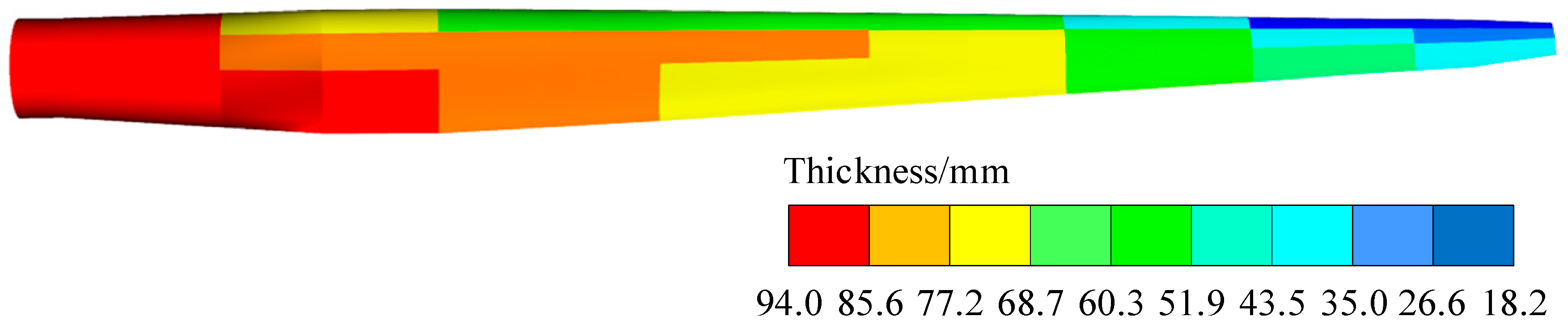
A three-dimensional geometric model of large wind turbine blades is established from the data on airfoil, propeller blade angle, and chord length.

(2)

Select the appropriate scale factor to calculate the wind turbine diameter, blade thickness, chord length, and other parameters, and use these to establish the geometric scale model.

(3)

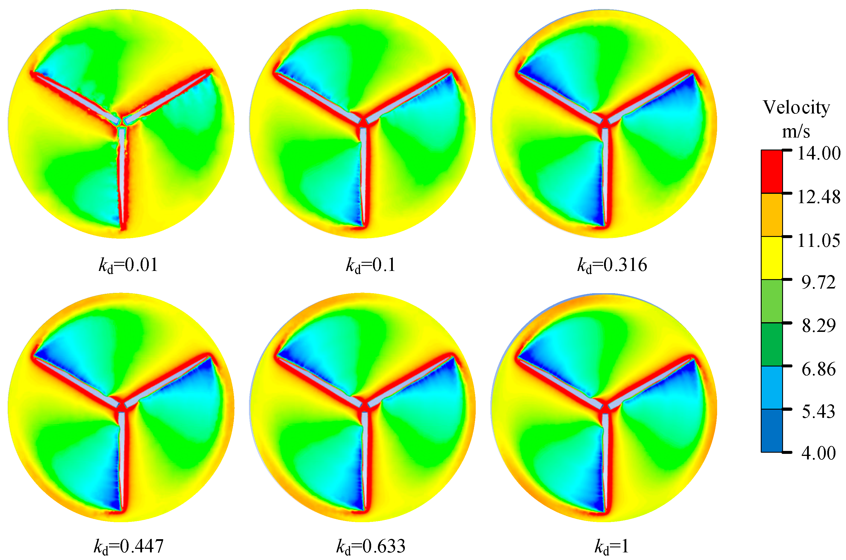
Under the premise that the flow pattern of the scaled model airfoil remains consistent with that of the prototype, the fluid dynamic simulation parameters, including the wind turbine incoming velocity, fluid medium density, and kinematic viscosity of the fluid medium, are determined.

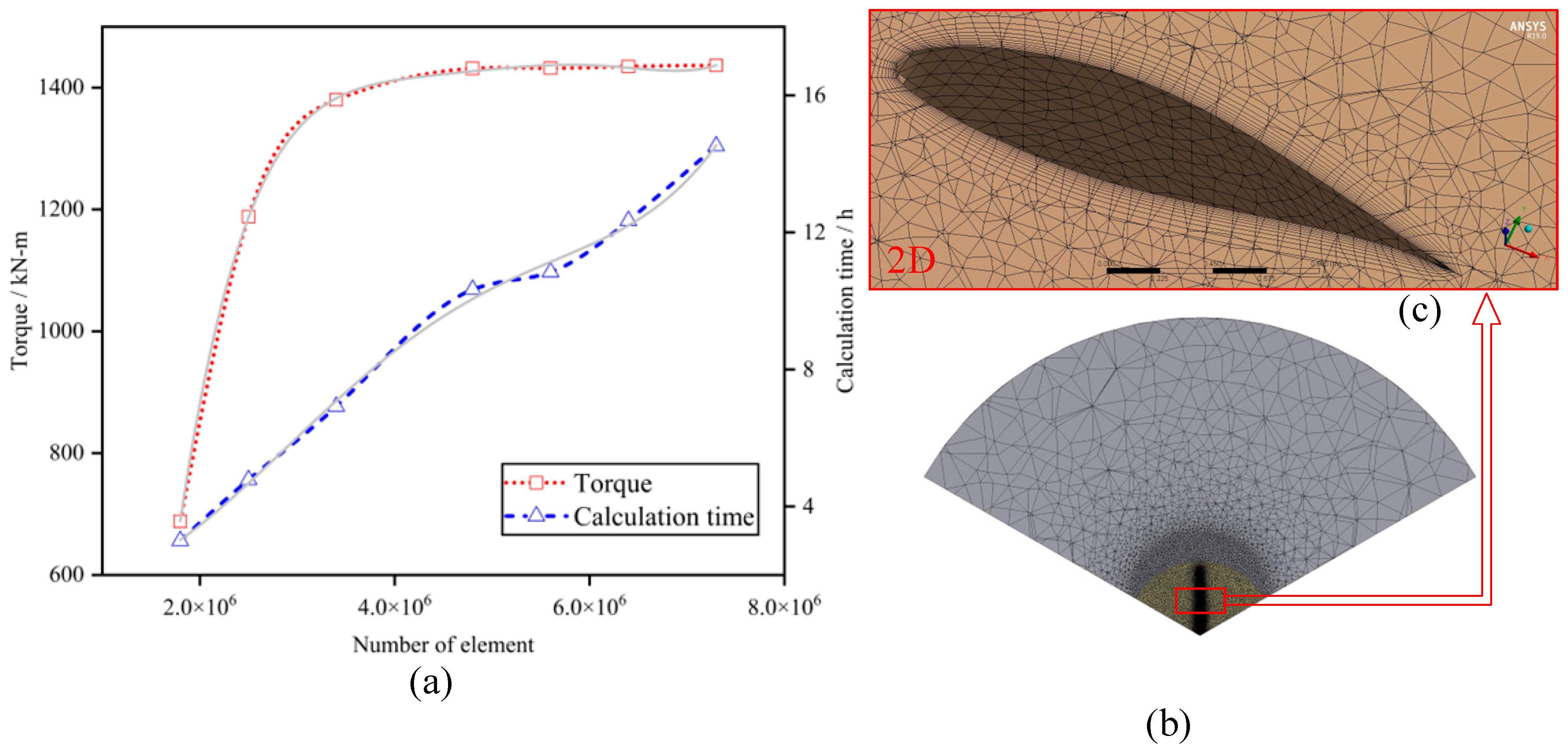
(4)

The wind rotor fluid domain model is constructed based on the geometric scaling relationship. The boundary layer thickness variation is calculated to determine the thickness of the first boundary layer, which is used to generate the fluid domain mesh model.

(5)

Given the inlet wind speed and the rotation speed of the wind turbine’s rotating domain, select an appropriate turbulence model to perform the fluid dynamic simulation analysis of the wind rotor. This process will provide the blade pressure distribution, from which the aerodynamic axial force and aerodynamic moment of the wind turbine blade can be calculated.

(6)

According to the material parameter scale factor, composite layups are performed on the wind turbine blade scale model. The structural design of the airfoil’s leading edge, trailing edge, spar, and web is completed using glass fiber, carbon fiber, balsa wood, and PVC foam.

(7)

Aerodynamic loads are applied to the blade surface, and static simulation analysis is performed to determine the deflection and stress–strain response of the scale model blade. The mechanical response of the blade prototype is evaluated using the blade structural response factor.

6. Numerical Examples

6.1. Blade Model

The wind turbine blade prototype used in this paper is the double-web blade of a 5 MW wind turbine published by NREL. The turbine has three blades, a hub diameter of 3 m, and a rotor diameter D of 126 m. The rated wind speed is 11.4 m/s, and the rated rotational speed is 12.1 rpm. Seventeen representative airfoil cross-sections of the blade are selected. These included seven typical shapes: circular, DU40_A17, DU35_A17, DU30_A17, DU25_A17, DU21_A17, and NACA64_A17. Composite materials are selected for the blade material, mainly BALSA foam, fiberglass, carbon fiber, and PVC foam. The density of PVC foam is 60 kg/m³, Young’s modulus is 48 MPa, and Poisson’s ratio is 0.45.

The mechanical property parameters of the composites are detailed in

Table 3. Mechanical properties of composite materials.

Name	Density kg·m−3	Ex MP	Ey MP	Ez MP	υxy -	υyz -	υxz -	Gxy MP	Gyz MP	Gxz MP
BALSA foam	80	2070	2070	4000	0.02	0.16	0.02	106	200	106
Two-way cloth glass fiber	1900	12,500	11,300	10,000	0.626	0.626	0.14	6000	6000	3200
Carbon fiber	1560	136,000	11,900	11,900	0.29	0.29	0.4	4860	4860	4400
One-way cloth glass fiber	1930	33,190	11,120	10,120	0.23	0.11	0.11	3690	3000	3000
Three-way cloth glass fiber	1910	24,700	13,700	9120	0.413	0.355	0.13	5200	5000	3000

. Based on the force analysis of the blade structure, the superior performance of the composite material in the direction of the glass fiber is optimized by reasonably selecting the layup angle, layup ratio, and layup order. At the blade root, the layup material is predominantly glass fiber in a three-way cloth with orientations of 0° and ±45°, which enhances its ability to withstand biaxial tensile and shear loads. The sandwich material is PVC foam. The primary layup material in the web is ±45° two-way cloth glass fiber, which enhances the shear resistance of the blades. The sandwich material is balsa wood. The layup material at the blade’s leading edge, spar, and trailing edge primarily consists of glass fiber in a three-way cloth with orientations of 0° and ±45°. PVC foam is used for the sandwich at the leading and trailing edges, while carbon fiber is employed for the spar and sandwich. Taking the 5 MW blade composite layup as an example, the layup thickness is illustrated in Figure 2. The thickness decreases along the blade’s span, with a maximum thickness of 94 mm at the blade root and a minimum thickness of 18.2 mm at the blade tip. The layup at the main beam and trailing edge is thicker than at the leading edge. The blade is a prototype to establish a three-dimensional geometric model with geometric scale factors of 0.01, 0.1, 0.316, 0.447, and 0.633. A blade geometry and material model is developed based on the relationship between these scale factors and the physical quantities of the scale model.

6.2. Aerodynamic Load

The analysis software is ANSYS. CFD is used to conduct the aerodynamic load analysis of wind turbine blades. The fluid domain model is constructed utilizing the multiple reference frame (MRF) approach. This method divides the flow field into external and internal fluid domains, with the rotation of the internal domain driving the fluid motion in the external domain, as illustrated in Figure 3. The surface of the internal domain is defined as the internal boundary condition. The velocity inlet and pressure outlet radius are set to 5 times the blade length. The velocity inlet is positioned 3 times the blade length from the plane of the wind rotor, while the pressure outlet is located 5 times the blade length from the blade. The radius of the internal flow field is set to 1.2 times the blade length. The external domain and internal domain interfaces are set as periodic boundary conditions to improve computational efficiency. The flow field domain is divided using an unstructured grid. To accurately capture the flow field dynamics, the thickness of the first boundary layer is set to 10⁻⁶ m, with 15 boundary layers employed.

Additionally, the grid density around the blades is increased to enhance accuracy. For the prototype wind turbine blade, the mesh size on the blade surface is set at 100 mm. Meshing is performed using a gradual encryption principle, moving from the inside to the outside, as illustrated in Figure 4. The Reynolds number of the atmospheric flow through the blade airfoil section is approximately 5.0 × 10⁷, the SST k-ω turbulence model is selected. Both momentum and turbulent kinetic energy are computed using second-order upwind schemes, while the pressure–velocity coupling is handled using the SIMPLE algorithm.

Based on the parameters outlined in Table 2, determine the operating environment parameters for the scale model wind turbine. Using the geometric scale as a reference, the finite element mesh generation for the scale model is performed, and the simulation analysis is conducted. For the prototype model, the velocity inlet for the incoming wind speed is set at 11.4 m/s, while the pressure outlet is maintained at atmospheric pressure. The wind wheel rotates at a speed of 12.1 rpm. For scaled models, the incoming wind speed is consistent with the prototype, for different geometric scaling factors of 0.01, 0.1, 0.316, 0.447, 0.633, and 1.0, with a wind turbine speed of 11.4/k_d. Aerodynamic load analysis should be carried out according to the proportional relationship between the axial force and torque of the scale model and those of the prototype. The results of these calculations are presented in

Table 4. Computational accuracy and efficiency of scale models.

Geometric Scale Factor kd	Theoretical Power kW	Total Number of Mesh -	Axial Force of Model N	Axial Force of Scale Model N	Torque of Model N·m	Torque of Scale Model N·m	Simulation Power kW	Calculation Time h
0.01	0.53	5.97 × 104	15.07	1.51 × 105	0.471	4.71 × 105	0.18	0.01
0.1	53.18	5.65 × 105	2346.84	2.35 × 105	1207.76	1.21 × 106	45.90	0.5
0.316	531.04	1.81 × 106	2.49 × 104	2.49 × 105	4.36 × 104	1.38 × 106	524.43	4.33
0.447	1062.59	2.29 × 106	5.02 × 104	2.51 × 105	1.25 × 105	1.39 × 106	1062.96	5.1
0.633	2130.87	2.97 × 106	1.01 × 105	2.52 × 105	3.57 × 105	1.41 × 106	2144.25	6.74
1.0	5318.02	4.80 × 106	2.58 × 105	2.58 × 105	1.43 × 106	1.43 × 106	5435.50	10.02

. For the prototype model, the torque calculated from the simulation is 1.43 × 10³ kN·m. Based on the relationship between unit power, torque, and wind turbine rotational speed, the wind turbine’s power at this point is 5.35 MW, which is close to its rated power of 5 MW. Additionally, the relative error compared to the measured torque of 1.41 kN·m reported in the literature is 1.4% [30]. As the geometric scale of the model decreases, the calculated axial force and torque of the scale model also decrease correspondingly. Meanwhile, the relative difference between the scaled axial force and torque compared to the prototype progressively increases. When the geometric scale is 0.316, the total number of meshes is 1.81 × 10⁶, and the relative differences in axial force and torque between the scale model and the prototype are 3.49% and 3.59%, respectively. The simulation time for the scale model is reduced to 4.33 h, which is half the calculation time required for the prototype. However, if the geometric scale is too small, significant errors may occur in the calculation results. For instance, at a geometric scale of 0.1, the blade length is 6.15 m, and the total number of meshes is 5.65 × 10⁵, resulting in relative differences in axial force and torque of 8.91% and 15.63%, respectively. At a geometric scale of 0.01, where the blade length is 0.615 m, and the total number of meshes is 5.97 × 10⁴, the relative differences in axial force and torque are 40.73% and 67.07%, respectively. When the geometric scale factor is less than 0.1, the error between the theoretical and simulated power increases significantly. For instance, at a scale factor of 0.01, the relative error is 66.04%. However, when the geometric scale factor exceeds 0.1, the relative error becomes smaller, indicating that selecting an appropriate scale factor enables the proportional model to achieve better accuracy. For example, at a scale factor of 0.447, the relative error between theoretical and simulated power is only 0.035%.

As the geometric scale factor decreases, the scaled model’s axial force and torque increasingly deviate from the prototype’s. To further clarify the discrepancy in calculation accuracy between the scaled model and the prototype, an analysis of the relative velocity distribution across the wind turbine plane is presented in Figure 5. The relative velocity distribution trend across the wind rotor plane for each scaled model is essentially consistent. The velocity on the rotor plane exhibits a stepped distribution, gradually decreasing along the direction of blade rotation. Near the blade’s leading edge, the maximum velocity reaches 14 m/s, while near the trailing edge, it decreases to a minimum of 4 m/s. When the geometric scale is larger than 0.1, the velocity distribution across each wind rotor plane remains largely consistent. However, when the geometric scale is reduced to 0.1 and 0.01, the velocity at the trailing edge of the blade significantly increases compared to the other models, and the velocity at the blade tip also rises substantially. This increase affects the velocity distribution around the blade tip and its periphery, decreasing pressure near the blade tip. According to BEM theory, the blade element segment near the tip experiences higher axial force and torque, which results in a notable discrepancy between the torque and axial force calculated by the scaled model.

The limiting streamlines on the suction surface of the blade for the scaled models are depicted in Figure 6. In all models, flow separation initiates from the blade’s root and intensifies at the transition section of the airfoil. This intensification leads to a stall vortex on the surface near the blade’s trailing edge, which subsequently expands along the blade’s span. The formation of stall vortices increases significantly as the geometric scale decreases. Except for the scale model with a geometric scale of 0.01, the region where flow separation is most pronounced lies between the blade root and the transition airfoil segment. After the transition airfoil section, the flow separation on the blade’s suction surface is markedly reduced, resulting in a fully attached flow state over the blade surface beyond the mid-span. Compared to the prototype, the scale models with geometric scales of 0.1 and 0.01 exhibit more extensive flow separation along the spanwise direction and generate more intense stall vortices. This phenomenon impacts the calculation of axial force and torque. In the mid-span section of the blade, the flow separation in these models slows down significantly, while in the rear section, the blade surface transitions to a fully attached flow state. A geometric scale that is too small in the model neglects the impact of the blade’s small features on the flow field due to the limitations in mesh size and total mesh count. This omission affects the velocity, pressure, and flow distributions around the blade and its periphery, leading to increased axial force and torque discrepancies between the scaled model and the prototype.

6.3. Static Analysis

Static analysis of the blade is a crucial method to verify whether the blade meets the strength and stiffness requirements. For different scale models, the scaling is performed according to the geometrical scale factor, applied along the blade span and airfoil thickness. The composite layup is scaled down for each layer’s thickness while maintaining the same layup angle as the blade prototype. When the blade is in a horizontal position, it is subjected to aerodynamic, gravitational, and inertia force loads. Considering the geometric nonlinear effect of the blade, the calculated blade deflection increases along the blade span, with the smallest deflection occurring at the root and the largest at the tip. The deflection and stress results for both the scale model and the prototype are presented in

Table 5. Computational accuracy of maximum deflection and equivalent stress of scale models.

Geometric Scale Factor kd	Maximum Deflection m	Maximum Deflection of Scale Model (m)	Maximum Equivalent Stress (N)	Relative Difference in Maximum Deflection (%)	Relative Difference in Maximum Equivalent Stress (%)
0.01	0.0091424	0.91424	9.1446 × 107	43.77	34.67
0.1	0.14688	1.4688	1.3374 × 108	9.67	4.46
0.316	0.48592	1.6016	1.4159 × 108	5.42	2.37
0.447	0.73806	1.6511	1.4567 × 108	1.53	3.91
0.632	1.0161	1.6078	1.4251 × 108	1.11	1.78
1	1.6258	1.6258	1.3998 × 108	-	-

. The table shows that as the geometric scale increases, the relative difference between the maximum deflection and maximum equivalent stress decreases. Specifically, when the geometric scale is 0.1, the relative difference in maximum deflection is 9.67%, and the relative difference in maximum equivalent stress is 4.46%. However, when the geometric scale is 0.01, these relative differences increase to 43.77% for maximum deflection and 34.67% for maximum equivalent stress.

6.4. Transient Analysis

During the rotation of the wind turbine blade, the gravitational force and the angle between the blade axis change cyclically with the azimuth angle position. This results in varying loads on the blade. This paper analyzes the loading conditions of the blade at two typical azimuthal positions: horizontal and vertical downward. An aerodynamic load is applied to the surface of the scaled model blade, which is then subjected to rotational movement from its highest point with a time step of 0.001 s. As the blade rotates, its spatial position is continuously updated, causing the aerodynamic load direction on the blade surface to be dynamically adjusted in real-time. Simultaneously, the structural response of the blade is calculated. The results of the calculations for the blade at rotational angles of 90° and 180° are presented in

Table 6. Computational accuracy and efficiency of blade rotation.

Geometric Scale Factor kd	Rotate 90° for Maximum Deflection m	Rotate 90° for Calculation Time h	Rotate 180° for Maximum Deflection m	Rotate 180° for Calculation Time h
0.01	0.9389	0.031	1.316	0.051
0.1	1.3102	0.117	2.147	0.26
0.316	1.3219	1.133	2.2032	2.48
0.632	1.3432	1.433	2.2462	3.75
1	1.3845	2.183	2.3451	6.95

. The maximum deflection is 1.38 m when the blade is rotated by 90°and 2.35 m when the blade is rotated by 180°. As the geometric scale factor increases, the relative difference in the maximum deflection also increases while the calculation time decreases. For a geometric scale factor of 0.316, the relative difference in maximum deflection is 4.52%, with a reduction in calculation time by 48.1%. For a scale factor of 0.1, the relative difference is 5.37%, with a reduction in calculation time by 94.64%. With a geometric scale factor of 0.01, the calculation time is reduced by 98.57%, but the relative difference in maximum deflection increases to 32.18%. The calculation accuracy and efficiency trend for a blade rotation of 180° follows a similar pattern to that observed for a 90° rotation.

To further analyze the reasons for the differences in the numerical accuracy of the scale model, the relative difference between the maximum deflection and the axial force is examined. This comparison is conducted for different blade rotation angles. The results are illustrated in Figure 7. As the geometric scale decreases, the relative difference between the three increases in the same direction. When the geometric scale reaches 0.01, the relative difference between the three reaches a maximum of more than 30%. Although the scale model with a geometric scale of 0.01 is rotated by 90° and 180°, the calculation efficiency is greatly improved compared with the prototype, but it cannot be used as a scale model to replace the prototype due to the significant relative difference of the axial force. When the geometric scale exceeds 0.1, the relative difference in axial force between the scale model and the prototype decreases significantly. The computational efficiency of the scale model improves observably compared to the prototype. Notably, the scale model with a geometric scale of 0.1 reduces the calculation time by up to 90% compared to the prototype.

7. Conclusions

In this paper, a scaled construction method for the numerical simulation of large wind turbine blades is proposed, based on fluid similarity and structural similarity criteria. This approach effectively reduces the calculation time for aerodynamic and structural simulations of large wind turbine blades. The main conclusions are as follows:

(1)

The proposed method ensures that the blade scale model satisfies structural and fluid similarities. This is achieved by coordinating the scale relationship of the model operation parameters, numerical simulation environment parameters, and mechanical response parameters.

(2)

The numerical scale model constructed can improve the efficiency of aerodynamic analysis and guarantee the solution’s accuracy by selecting appropriate geometric scale factors. For a geometric scale factor of 0.316, the relative difference in maximum deflection is 4.52%, with a reduction in calculation time by 48.1%.

(3)

The scale model is suitable for aerodynamic load analysis, structural static analysis, and structural transient analysis, and the precision of the scale model is mainly related to the accuracy of aerodynamic analysis.

8. Future Work

The numerical simulation model presented in this paper significantly improves the computational efficiency of static aerodynamic load analysis; however, the accuracy of the calculations decreases noticeably when the scale factor is less than 0.1. With the growing trend of high-power wind turbines, the lightweight design of turbine blades remains a critical challenge in blade engineering. While the method proposed here enhances the computational efficiency of aerodynamic load analysis by fivefold, and transient analysis by nearly tenfold, achieving lightweight designs for large wind turbine blades in the near future remains difficult. Addressing this challenge will be the focus of our future work.

References

1. Ben Backwell, M.H.; Khinda, N.; Clarke, E.; Qiao, L.; Williams, R.; Tan, W.H.; Liang, W.; Esther, A.L.; Fang, M.R.; Ann Margret, T.V.B.; et al. Global Wind Report 2024; 2024. Available online: https://gwec.net/global-wind-report-2024/ (accessed on 16 April 2024).
2. Ghiasi, P.; Najafi, G.; Ghobadian, B.; Jafari, A.; Mamat, R.; Ghazali, M.F. CFD-Study of the H-Rotor Darrius wind turbine performance in Drag-Lift and Lift Regime: Impact of type, thickness and chord length of blades. Alex. Eng. J. 2023, 67, 51–64. [Google Scholar] [CrossRef]
3. Hijazi, A.; ElCheikh, A.; Elkhoury, M. Numerical investigation of the use of flexible blades for vertical axis wind turbines. Energy Convers. Manag. 2024, 299, 117867. [Google Scholar] [CrossRef]
4. Eltayesh, A.; Castellani, F.; Burlando, M.; Hanna, M.B.; Huzayyin, A.; El-Batsh, H.M.; Becchetti, M. Experimental and numerical investigation of the effect of blade number on the aerodynamic performance of a small-scale horizontal axis wind turbine. Alex. Eng. J. 2021, 60, 3931–3944. [Google Scholar] [CrossRef]
5. Khalafallah, M.G.; Ahmed, A.M.; Emam, M.K. The effect of using winglets to enhance the performance of swept blades of a horizontal axis wind turbine. Adv. Mech. Eng. 2019, 11, 1687814019878312. [Google Scholar] [CrossRef]
6. Zheng, T.; Zhao, C.; He, J. Research on Fatigue Performance of Offshore Wind Turbine Blade with Basalt Fiber Bionic Plate; Structures 2023; Elsevier: Amsterdam, The Netherlands, 2023; pp. 466–481. [Google Scholar]
7. Hand, B.; Kelly, G.; Cashman, A. Structural analysis of an offshore vertical axis wind turbine composite blade experiencing an extreme wind load. Mar. Struct. 2021, 75, 102858. [Google Scholar] [CrossRef]
8. Rezaei, M.M.; Behzad, M.; Moradi, H.; Haddadpour, H. Modal-based damage identification for the nonlinear model of modern wind turbine blade. Renew. Energy 2016, 94, 391–409. [Google Scholar] [CrossRef]
9. Chen, Y.; Griffith, D.T. Blade mass imbalance identification and estimation for three-bladed wind turbine rotor based on modal analysis. Mech. Syst. Signal Process. 2023, 197, 110341. [Google Scholar] [CrossRef]
10. Jayswal, S.; Bhattu, A. Structural and modal analysis of small wind turbine blade using three different materials. Mater. Today Proc. 2023, 72, 1347–1352. [Google Scholar] [CrossRef]
11. Navadeh, N.; Goroshko, I.; Zhuk, Y.; Etminan Moghadam, F.; Soleiman Fallah, A. Finite element analysis of wind turbine blade vibrations. Vibration 2021, 4, 310–322. [Google Scholar] [CrossRef]
12. Lipian, M.; Czapski, P.; Obidowski, D. Fluid-structure interaction numerical analysis of a small, urban wind turbine blade. Energies 2020, 13, 1832. [Google Scholar] [CrossRef]
13. Marzec, Ł.; Buliński, Z.; Krysiński, T. Fluid structure interaction analysis of the operating Savonius wind turbine. Renew. Energy 2021, 164, 272–284. [Google Scholar] [CrossRef]
14. Li, J.; Liu, R.; Yuan, P.; Pei, Y.; Cao, R.; Wang, G. Numerical simulation and application of noise for high-power wind turbines with double blades based on large eddy simulation model. Renew. Energy 2020, 146, 1682–1690. [Google Scholar] [CrossRef]
15. Maizi, M.; Mohamed, M.; Dizene, R.; Mihoubi, M. Noise reduction of a horizontal wind turbine using different blade shapes. Renew. Energy 2018, 117, 242–256. [Google Scholar] [CrossRef]
16. Moon, H.; Jeong, J.; Park, S.; Ha, K.; Jeong, J.-H. Numerical and experimental validation of vortex generator effect on power performance improvement in MW-class wind turbine blade. Renew. Energy 2023, 212, 443–454. [Google Scholar] [CrossRef]
17. Siddiqui, M.S.; Rasheed, A.; Kvamsdal, T.; Tabib, M. Quasi-static & dynamic numerical modeling of full scale nrel 5mw wind turbine. Energy Procedia 2017, 137, 460–467. [Google Scholar]
18. Zhang, Y.; Song, Y.; Shen, C.; Chen, N.-Z. Aerodynamic and structural analysis for blades of a 15MW floating offshore wind turbine. Ocean Eng. 2023, 287, 115785. [Google Scholar] [CrossRef]
19. Gao, G.; Wang, H.; Li, E.; Li, G. An exact block-based reanalysis method for local modifications. Comput. Struct. 2015, 158, 369–380. [Google Scholar] [CrossRef]
20. Jokar, H.; Mahzoon, M.; Vatankhah, R. Nonlinear dynamic characteristics of horizontal-axis wind turbine blades including pre-twist. Ocean Eng. 2022, 256, 111441. [Google Scholar] [CrossRef]
21. Kim, H.; Lee, S.; Son, E.; Lee, S.; Lee, S. Aerodynamic noise analysis of large horizontal axis wind turbines considering fluid–structure interaction. Renew. Energy 2012, 42, 46–53. [Google Scholar] [CrossRef]
22. Zhang, D.; Liu, Z.; Li, W.; Hu, G. LES simulation study of wind turbine aerodynamic characteristics with fluid-structure interaction analysis considering blade and tower flexibility. Energy 2023, 282, 128840. [Google Scholar] [CrossRef]
23. Hu, Z.; Dang, C.; Wang, L.; Beer, M. Parallel Bayesian probabilistic integration for structural reliability analysis with small failure probabilities. Struct. Saf. 2024, 106, 102409. [Google Scholar] [CrossRef]
24. Chasapi, M.; Antolin, P.; Buffa, A. Fast parametric analysis of trimmed multi-patch isogeometric Kirchhoff-Love shells using a local reduced basis method. Eng. Comput. 2024, 1–28. Available online: https://link.springer.com/article/10.1007/s00366-024-01980-6 (accessed on 24 September 2024). [CrossRef]
25. Teng, D.; Feng, Y.-W.; Lu, C.; Keshtegar, B.; Xue, X.-F. Generative adversarial surrogate modeling framework for aerospace engineering structural system reliability design. Aerosp. Sci. Technol. 2024, 144, 108781. [Google Scholar] [CrossRef]
26. Li, W.; Chen, S. Structural reanalysis method for local modifications based on system reduction and iterative solution. Eng. Struct. 2022, 273, 114977. [Google Scholar] [CrossRef]
27. Luo, T.; Wu, G.; Zhang, P.; Zhang, H. A new similarity criterion for wind tunnel testing of floating wind turbines achieving dynamic aerodynamic characteristics similarity. Energy Convers. Manag. 2024, 301, 118015. [Google Scholar] [CrossRef]
28. Wang, X.; Cai, C.; Chen, Y.; Chen, Y.; Liu, J.; Xiao, Y.; Zhong, X.; Shi, K. Numerical verification of the dynamic aerodynamic similarity criterion for wind tunnel experiments of floating offshore wind turbines. Energy 2023, 283, 129082. [Google Scholar] [CrossRef]
29. Tschepe, J. On the prediction of boundary layer quantities at high Reynolds numbers. Fluids 2022, 7, 114. [Google Scholar] [CrossRef]
30. Jonkman, J.; Butterfield, S.; Musial, W.; Scott, G. Definition of a 5-MW Reference Wind Turbine for Offshore System Development; Technical Report No. NREL/TP-500-38060; National Renewable Energy Laboratory: Golden, CO, USA, 2009. [Google Scholar]
Figure 1. Construction and analysis of wind turbine blade scale numerical model.
Energies 17 04849 g001
Figure 2. Thickness of composite materials for 5 MW blade.
Energies 17 04849 g002
Figure 3. Flow field under multiple reference frames.
Energies 17 04849 g003
Figure 4. Mesh Independence Validation. (a) Grid independence verification. (b) Flow field meshing. (c) Boundary layer grid.
Energies 17 04849 g004
Figure 5. Plane velocity of wind rotor of scale models.
Energies 17 04849 g005
Figure 6. Limit streamline diagram of suction surface of scale models.
Energies 17 04849 g006
Figure 7. Relative differences under transient conditions.
Energies 17 04849 g007