Abstract
Solar energy plays a major role in the transition to renewable energy. To ensure that large-scale photovoltaic (PV) power plants operate at their full potential, their monitoring is essential. It is common practice to utilize drones equipped with infrared thermography (IRT) cameras to detect defects in modules, as the latter can lead to deviating thermal behavior. However, IRT images can also show temperature hot-spots caused by inhomogeneous soiling on the module’s surface. Hence, the method does not differentiate between defective and soiled modules, which may cause false identification and economic and resource loss when replacing soiled but intact modules. To avoid this, we propose to detect spatially inhomogeneous soiling losses and model temperature variations explained by soiling. The spatially resolved soiling information can be obtained, for example, using aerial images captured with ordinary RGB cameras during drone flights. This paper presents an electrothermal model that translates the spatially resolved soiling losses of PV modules into temperature maps. By comparing such temperature maps with IRT images, it can be determined whether the module is soiled or defective. The proposed solution consists of an electrical model and a thermal model which influence each other. The electrical model of Bishop is used which is based on the single-diode model and replicates the power output or consumption of each cell, whereas the thermal model calculates the individual cell temperatures. Both models consider the given soiling and weather conditions. The developed model is capable of calculating the module temperature for a variety of different weather conditions. Furthermore, the model is capable of predicting which soiling pattern can cause critical hot-spots.
1. Introduction
To achieve net zero greenhouse gas emissions by 2050, a global energy system transformation is vital. At the forefront, solar and wind will account for the largest share of renewable energy sources [1,2]. This development can already be seen in the continuously growing cumulative installed photovoltaic (PV) capacity worldwide [3]. Large-scale PV power plants play an important role. Monitoring their performance becomes essential to maintain the highest possible power output, as modules may become defective or soiled.
Defective modules can show mechanical damage, thermal damage, or manufacturing errors [4]. Specific examples are cell cracks, burn marks, or defective bypass diodes [5]. These failures cause power production decreases and consequently, income losses. Therefore, the replacement of defective modules should be considered. Furthermore, defects can lead to hot-spots and even cause security issues. Hot-spots are locations within a PV module that show a temperature increase compared to the remaining PV module’s surface. However, hot-spots are typically not defined by the temperature increase exceeding a certain threshold. Instead, a hot-spot is typically defined as a cell being operated with a current higher than its short-circuit current. This causes the affected cell to be operated in the reverse bias region and thus leads to power dissipation and local heating [6].
Soiled PV modules are modules that have accumulated dust, pollen, and other contaminants on the module surface [7]. As a layer of soiling prevents parts of the incoming solar radiation from reaching the PV cell, less energy is converted into electricity [8]. This results in power loss due to soiling, income loss, and accelerated degradation [9,10]. On a global average, power losses are assumed to be around 4–7%, and income losses are estimated at EUR 3–5 billion per year [11]. Certain countries exhibit even higher annual power losses due to soiling, as Maghami et al. [12] found in a comparative analysis. The modules should therefore be cleaned in many cases. Homogeneous soiling affects a module’s behavior similar to a change in incoming solar radiation [7,13]. In this case, the electrical losses in terms of output power are approximately equal to the optical losses. However, inhomogeneous soiling can be critical as it generally leads to higher electrical losses and potentially causes hot-spots which in turn can cause various operating faults. Bird droppings and leaves are examples of inhomogeneous soiling. Power losses caused by inhomogeneous soiling are at times much higher than the corresponding optical losses [12]. This is related to the electrical properties of the module. Cells are connected in series and the maximum current of the affected string is limited by the soiled cell. This effect is referred to as electrical mismatch [14]. In severe cases, the heaviest soiled cell dissipates parts of the energy generated by the lesser soiled cells [14]. As a result, the affected cell heats up compared to its neighbors. This can lead to the formation of hot-spots.
If hot-spots are detected, it can be difficult to determine their origin. A distinction between hot-spots on defective and soiled modules is desired. Infrared thermography (IRT) has emerged as a typical approach to detect hot-spots in general for both defective and soiled modules via analyzing the temperature distribution of the modules. However, as both defective and soiled PV cells heat up, the IRT images show the same qualitative behavior for both cases [4,9]. This is illustrated in Figure 1 and Figure 2. The temperature deviations in the IRT image seen for defects (Figure 1) and artificial shading/soiling (Figure 2) are similar and it is not directly clear from the ITR images if the modules are defective. Additional electroluminescence measurements shown in Figure 3 can confirm that the module from Figure 1 indeed has several defects.
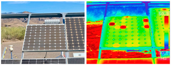
Figure 1.
(Left): RGB image of a defective module. On the RGB image it appears clean, and a potential hot-spot is not observed. (Right): IR image of the defective module. The IR image clearly shows 4 hot cells. By having access to both the RGB and the IR images, one can conclude that the module is defective. One string, the third and fourth column from the right, is bypassed. The temperature is slightly increased compared withthe other cells (except of the hot-spots).
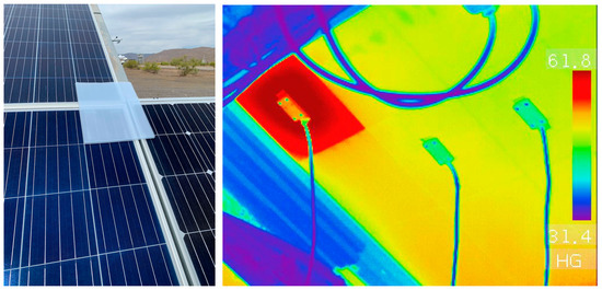
Figure 2.
(Left): RGB image of the artificially shaded/soiled cell. (Right): IR image of the rear side of the PV module seen in the RGB image on the left. The artificially shaded cell shows a significant temperature increase (hot-spot).
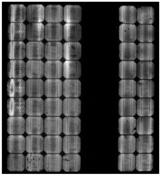
Figure 3.
Electroluminescence image of the above-mentioned module. There are multiple cracks visible. This module is likely to show one or more hot cells when operated. One string is bypassed and therefore shows no electroluminescence signal.
In summary, IRT does not directly differentiate between defective and soiled modules. This potentially causes false identification and might lead to the obsolete cleaning of defective modules, unnecessary additional measurements after the detection of the heated areas (e.g., electroluminescence), or the unnecessary replacement of soiled but intact modules. These measures represent an avoidable effort.
One way to overcome this problem is to distinguish between defective and soiled PV modules in an automatized way using optical and IR images. Costs are reduced by the avoidance of unnecessary replacements and manual checks on site alike. Additionally, losses due to lower energy production and thus lower revenues are avoided. To this end, we propose to not only rely on drone flyovers for IRT to detect defective modules but also to additionally assess the inhomogeneous soiling of the PV module. Such soiling data can be captured, for example, using optical RGB images [15]. RGB images have been used to calculate cell-resolved soiling losses for dust-like soiling. Other studies have also investigated dust [16,17] as well as snail trails [18]. The latter three studies have a practical shortcoming in that they do not state the electrical loss caused by the soiling.
In this study, the soiling data are processed in sequence with an optical, electrical, and thermal model to obtain a second temperature map reflecting the expected temperature of a PV module without any defect, but with the measured spatially resolved soiling loss. The combination of the optical and electrical models determines if the soiling distribution is indeed sufficient to cause a hot-spot and deliver the expected cell temperature.
The modeled temperature map is then compared to the measured one from the IRT camera that reflects both soiling and defects. In case the IRT image shows a hot-spot, but the modeled temperature map does not, the hot-spot is caused by a defect. When IRT images show a hot-spot and the modeled temperature map also shows a hot-spot for the same cell, the soiling is likely the origin of the hot-spot. In this case, however, it is possible that in addition to the local soiling, a defective cell is also present. If the hot-spot persists after appropriate cleaning, it can be concluded that the cell is defective.
This approach allows us to determine which modules need to be replaced and hence avoid false identification and the replacement of intact modules. The required extra effort is to additionally measure and evaluate the soiling pattern, using the here-presented model and, e.g., RGB images, which many IR camera systems can capture in parallel to the IR images anyway.
Cipriani et al. have developed a Convolutional Neural Network (CNN) that is capable of distinguishing anomalies observed in IR images in two categories, “dust” and “fault” [19]. The accuracy of this classification was 98% for the tested cases. This distinction comes close to the desired one described above, but it is not the same. The authors used the terms “hot-spot” and “fault” interchangeably because there was no soiling that was so intense that it could cause a hot-spot in their dataset. At the same time, “dust” is considered to be a different anomaly on the IR images that does not cause a hot-spot. This means that the method presented by Cipriani et al. cannot distinguish between hot-spots caused by soiling and hot-spots caused by defects. This separation is the objective of our work.
This paper is structured as follows. First, an overview of the state of the art is given in Section 2. Different existing thermal models and monitoring methods are discussed. Then, the developed electrothermal model is explained in detail in Section 3. The experimental setup and the validation of the electrical and thermal results of the model are discussed in Section 4. Finally, a summary is made and an outlook is given in Section 5.
2. The State of the Art
There are various approaches for the temperature of PV modules. Some models focus on providing a single module temperature. This means that these models implicitly assume the module to be clean or homogeneously soiled, the cells and the module to be fully intact, and hence the temperature to be homogeneous. Their advantage is that they are easy to implement and involve a low computational effort. Other models focus on calculating the hot-spot temperature that can arise when a cell of a module experiences a certain degree of shading. Typically, the models consider either the entire area of a cell to be covered with a layer of a certain transmittance or a certain area of a cell to be covered with a completely opaque layer. The latter category of studies shows methods to calculate the hot-spot temperature of defective cells. Typically, these models are structured in the following way. The models are only applied if a hot-spot is detected on an IRT image. After observing the hot-spot, its temperature distribution is calculated. These defects, which are typically shunts, cannot be predicted by the model. These methods therefore require an IR image for the temperature calculation. We are going to use RGB images to calculate the temperature. Later, we want to compare our calculated temperature against the IR image. In contrast to other thermal models from the literature, the IR image is not used as an input for the electrothermal model.
2.1. Thermal Models
There are several previously published models to estimate the PV cell temperature. Such models consider the incoming solar radiation, the wind speed, the ambient temperature, the relative humidity, soiling (either measured or estimated), and the load resistance [20,21,22]. Several studies show that the cell temperature is a particularly important factor for predicting a PV module’s efficiency as a temperature increase of 1 K typically causes a relative reduction in efficiency at around 0.4% for silicon modules [23,24,25].
One of the simplest thermal models is the Ross model [26]. The Ross model is defined in Equation (1) and determines the cell temperature . The model requires the following input parameters: the ambient temperature , the global tilted irradiance , and the module’s NOCT (normal operating cell temperature) . The NOCT is stated by the manufacturer in the data sheet. It considers the following conditions: GTI = 800 W/m2, wind speed = 1 m/s, ambient temperature = 20 °C, and air mass 1.5.
Note that for all equations in this section, the temperatures are considered in °C and the irradiances are considered in W/m2.
The Sandia Photovoltaic Array Performance Model [27] considers wind effects. In the first step, the model determines the PV module’s backside temperature and the surface temperature on the module’s rear side, . In the second step, it calculates the cell temperature . The Sandia model requires the , two empirically determined coefficients and based on the module structure and the type of mounting, the wind speed , and the ambient temperature . Equation (2) shows how to determine the backplate temperature and the cell temperature , respectively. Note that describes the temperature difference between and for a of 1000 W/m2. has the unit and b has the unit .
The Faiman model is a thermal model which uses empirical heat loss factors [28]. Equation (3) describes how the cell temperature is determined based on the ambient temperature , the , the two heat loss factors and , and the wind speed .
The U.S. National Renewable Energy Laboratory developed the NOCT Cell Temperature Model as part of the System Advisor Model (SAM) [29]. It is one of the most sophisticated thermal models. Equation (4) illustrates how the thermal model predicts the cell temperature . Input variables are the ambient temperature , the , and the module efficiency at reference conditions. In addition, the effective transmittance–absorbance product is required, which combines the transmittance and absorptance effects of the photovoltaic cell with the incoming solar radiation . Both and are adjusted by the type of mounting and the height above the ground leading to and . To obtain these parameters, an offset is added to , and is multiplied by an attenuation factor [29].
These thermal models consider the ambient temperature and solar radiation to determine cell temperatures. Three of them also include wind speed, which is expected to have a major impact on the results [13,30]. Yet, the thermal models lack in replicating the whole PV module under partial shading or partial soiling conditions. Even though single cells can be simulated and their temperatures determined on the cell level, the effects of shaded cells on their neighboring cells and the entire surrounding string are not considered. However, this would be necessary for our purpose.
2.2. Modeling of Hot-Spots
Qian et al. have developed a model that is capable of simulating the hot-spot temperature of a partially shaded cell [31]. They have investigated different degrees of shading, changing the covered area of a given cell. A key finding was that half-cell modules are less prone to create hot-spots. If a hot-spot occurs, the temperature increase will be significantly lower compared with an analogous full-cell module. The developed model was not validated against a measurement. The model was not designed to be applied in outdoor conditions. Instead, the estimation of the above-mentioned difference between half-cell and full-cell modules was the objective. Solheim et al. have simulated a PV hot-spot accurately using a finite elements method [32]. They considered 800,000 nodes per module. This makes the approach too intense in terms of calculation to be applied to a larger scale. A study by Rossi et al. presented a thermal model that is not only capable of estimating the final hot-spot temperature, but that is also capable of modeling the process of the affected cell heating up over time [33]. It is a dynamic model instead of a steady-state model. Furthermore, the paper proposed a method to detect hot-spots. The hot-spot detection relies on current sensors connected to the output of each module. It is desirable to use images for hot-spot detection as this would remove the need of the above-mentioned current sensors. The current sensors would offer the advantage of permanently providing data. A drone camera system would not have this advantage. Surveillance cameras can continuously record data. The thermal model has not been validated under outdoor operating conditions. Geisemeyer at al. developed a thermal model that is capable of calculating the hot-spot temperature of a partially shaded cell [34]. Their model not only gives a value of the temperature, but it also gives the temperature distribution within the affected cell. On the other hand, their model is very complex and unsuitable to be applied to a larger number of modules.
To the best of our knowledge, there is no thermal model with low calculation effort for hot-spot temperature simulation of soiled or shaded cells that is validated over a larger time interval under real operating conditions that uses only the cell-resolved soiling and meteorological data as inputs.
This paper aims to develop a simple enough electrothermal model that is usable for real operating conditions and the specific application case with cell-resolved soiling input data that provides the temperature output with cell resolution. In particular, the electrothermal model is connected to the cell-resolved soiling measurements from [15,35].
3. Description of the New Electrothermal Model
3.1. Thermal Model
The thermal model developed in this work is illustrated in Figure 4. It has a structure of four layers and six temperature nodes. The four layers are the soiling layer, the front glass cover, the silicon layer, and the backplate. The temperature nodes are , the temperature of the upper side of the soiling layer , the temperature of the upper side of the glass layer , the silicon temperature (subscript c referring to the cell), the temperature of the lower side of the backplate , and the ground temperature (subscript f for the floor). Note that we consider the silicon layer to be much thinner than the other layers. Roughly, the silicon layer should be around 300 µm [36]. By making this assumption we can assume that there is only one cell temperature, and the cell has no thermal resistance. Note also that the description of a PV cell as a stack of three layers is generally a big simplification. The goal is to develop an easily usable thermal model. The goal is not to predict the temperature with sub-digit precision. Furthermore, the back reflector is neglected because of its thickness of around 20 µm [37]. Thin passivation layers are also not considered here.
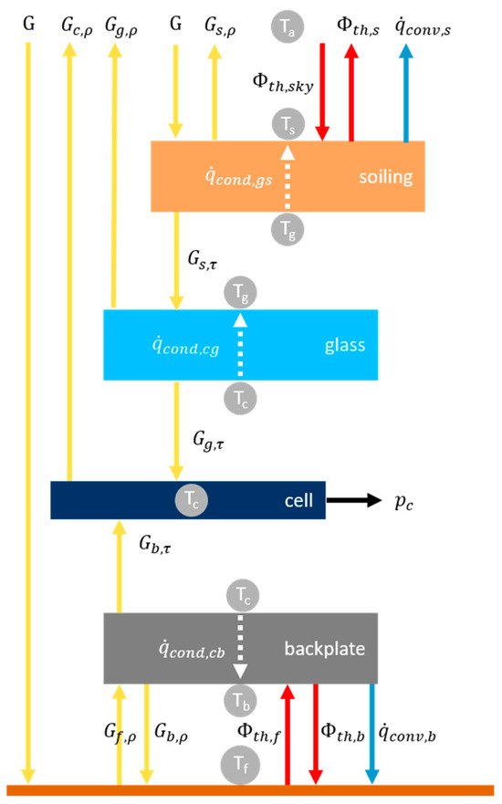
Figure 4.
Sketch of the model structure. Shown are the four different layers of the model and the temperature nodes. Additionally, all energy fluxes are illustrated.
Note furthermore that out of the six above-mentioned temperatures, the ambient temperature and the ground temperature are inputs while the other four are outputs of the model. is measured with a CS215-L thermometer (Hinesburg, VT, USA). has been estimated to be 10 K colder than the ambient temperature. This assumption is connected with uncertainties. However, it has been confirmed that the resulting variations in , if had a 10 K uncertainty, are one order of magnitude smaller than the convective heat transfer on the rear side for the case of a non-hot-spot and two orders of magnitude smaller for the case of a hot-spot. In the future, the simplest method would be to measure the floor temperature. There are also various approaches to model the ground temperature [38,39,40]. However, for our purposes, they are less suitable as they are quite complex by themselves and generally require many inputs. Furthermore, the floor temperature is not going to be spatially homogeneous as the ground experiences a shading pattern that changes over time. Additionally, the ground and the module’s rear side are not parallel to each other. Therefore, the rear side in reality does not receive the entire thermal radiation emitted by the ground. Instead, it should receive a weighted average of and .
Energy fluxes in between the four layers and the surroundings can be divided into five categories: GTI , thermal radiation , thermal conduction , convection , and generated surface power density . The surface power density is defined as the electrical power generated by the PV cell, divided by the cell area . The GTI is measured by a reference cell in the wavelength range from 400 nm to 1150 nm. According to the manufacturer, the relative deviations against class pyranometers are up to 5%. The thermal radiation of the sky is measured by a pyrgeometer (see Table 1). The pyrgeometer roughly starts to measure at 4 µm until 100 µm. The thermal radiation of the sky could also be estimated with a weather model in case there is no pyrgeometer available. The other fluxes are not measured and are only intermediate results for the model.

Table 1.
Overview of the origin of the known parameters for the thermal model.
The thermal radiation emitted by the soiling layer is denoted as . is the thermal radiation emitted by the floor and is the thermal radiation emitted by the back sheet.
is the part of that is transmitted through the soiling layer. is the part of that is reflected at the soiling layer or, in other words, scattered back to the air above the soiling layer. As for the soiling layer, reflection and transmission can take place at each interface between the layers. is the part of that is transmitted through the glass layer. is the part of that is reflected at the interface between the soiling layer and the glass layer. Reflections of second order are neglected here. For example, can be reflected again at the interface between glass and soiling, but we work without this term as a simplification. is the part of the GTI that reaches the back sheet of the module. Attenuations occur because the module itself is shading the ground. A part of the light that reaches the ground is reflected, both directly and diffusively. Finally, only a fraction of the reflected light reaches the module’s rear side. The ground albedo and the view factor have to be considered for . The view factor describes the fraction of the light reflected by the unshaded area that reaches the module’s back sheet. is the part of that is transmitted through the back sheet and is the part that is reflected there.
is the conductive heat transfer through the soiling layer. is the conductive heat transfer through the glass layer. is the conductive heat transfer through the back sheet. All conductive heat transfers point away from the cell. This is defined this way because the cell is the layer that absorbs the most radiation and is therefore the hottest. is the convection that takes place on the soiled surface. is the convection that takes place on the rear side of the module.
is the power density generated by the cell which describes the electric power exiting the cell (positive sign) or the received electric power converted to heat (negative sign). All quantities are defined in such a way that they are positive for common operating conditions without a hot-spot.
Assuming steady-state temperatures and considering each layer by itself, input and output fluxes can be equated in the form of balance equations. The balance equations for each layer are shown in Equations (5)–(8). The order of the equations is the same as the one of the layers shown in Figure 4.
Equations (9)–(11) describe how the thermal radiation, the thermal conduction, and the convection depend on the temperature, respectively. For thermal radiation, the key parameters are the body’s emissivity , the Stefan–Boltzmann constant , and the body’s surface temperature . The thermal conduction depends on the thermal conductivity , the temperatures of hot and cold sides and , and the corresponding thickness . Convection depends on the temperature difference between the surface and the ambient temperature and the convective heat transfer coefficient , which depends on the windspeed itself.
Both free and forced convection are considered. The heat transfer coefficients are combined as the square root of the quadratic sum [50]. In some cases, larger exponents instead of two might be used. Notton et al. discuss a few different forced and free convection models for PV modules [45]. We use the free convection model by [51] and the forced convection by [52]. See, therefore, Equations (12) and (13). Equation (14) shows how free and forced convection are combined. Roughly speaking, for windspeeds above 3 m per second the forced convection dominates. vice versa for windspeeds below 1 m per second, the free convection can be interpreted as a lower limit.
is the characteristic length of the module, which in this case is the module height. is the inclination of the module. and are the module temperature and the ambient temperature, like in the literature models discussed above.
We derive the air parameters from the US Standard Atmosphere [49]. Some parameters are estimated involving certain assumptions. For example, we assume that there is no transmission through the cell, meaning we neglect UV and IR radiation passing through the semiconductor layer. The error we make by making this assumption should be of the same order of magnitude as the neglect of multiple reflections. For the convection, some parameters are also determined using the Python library fluids [53], which contains functions of the US Standard Atmosphere [49]. Other parameters are derived from the data sheet of the PV module [48]. The physical properties of each layer will be discussed in Section 3.2.
3.2. Material Properties of Layers
We selected a set of material properties based on the literature and the module data sheet. This set includes optical properties such as reflectance, transmittance, and emissivity. The parameter set also includes the thermal conductivity. In addition, the layer thickness is stated. All parameters are illustrated in Table 2. If there are multiple values for one parameter, the one emphasized in bold was finally implemented in the thermal model. The * symbol indicates that the value is an assumption with justification in the caption of this table. The emissivity of silicon is not stated here because thermal radiation only takes place at surfaces, i.e., at the interfaces with air. In our model, the silicon layer is therefore not emitting thermal radiation. The thermal conductivity of silicon is not stated because the silicon layer is assumed to be thin against the glass and backplate layers. The absorptance of each layer is not stated here as it can be calculated simply, as the sum of reflectance, transmittance, and absorptance has to be one. The transmittance through the semiconductor layer itself is neglected. The literature states that the fraction of the light that is transmitted through the silicon layer is in the low single-digit percent range. Additionally, most parts of this light are then reflected at the back reflector, which has not been included in our model. Note also that the thickness of a dust layer will be different in each situation. A reasonable dust particle diameter is 10 µm [11,54]. Since there is no significant thermal resistance in such a thin layer, this thickness can be neglected. The dust surface temperatures and the module surface are basically the same.
Table 2.
This table summarizes the most important properties of the four module layers. If there are multiple values stated for a parameter, the value in bold is chosen. (*) indicate approximations. The explanations are given in the text.
For the ground, we assumed an emissivity of 0.947 [56]. The albedo of the ground was 0.189 [62]. We assumed that 5% of the incident light would be reflected and reach the rear side of the module. This could only be estimated as parts of the ground were shaded by the module itself. Also, not the entire part that was reflected at the ground went in the direction of the module. The larger part went toward the rest of the hemisphere.
The soiling layer’s parameters were estimated as follows. The most important property was the transmittance as it determines whether the cell generates or dissipates energy. For dust-like soiling, one can assume that reflection and scattering dominate over absorption [11]. For other soiling types, considerations have to be made individually. In our experiments, we used a stack of foils which would also have a very low absorptance. For the experiments presented in Section 4.2, the transmittance of the foils were measured optically with a Perkin Elmer Lambda 1050 spectrophotometer (see Appendix A). In the future, the transmittance model developed in [,35] can determine the transmittance of dust using RGB images of the affected modules. In terms of the emissivity, there is the literature for both: the plastic foils used here and for mineral dust, which is a future application. Ground reflectance, i.e., the albedo, is also a prerequisite for the precise determination of the energy balance [63]. The ground emissivity varies depending on the ground type. For instance, the bare soil calcaric regosol shows an emissivity of 0.947, whereas green-colored short grass has a higher emissivity of 0.976 and dry grassland reaches a value as high as 0.99 [56]. Finding an accurate value that suits our testbench was less important because only a fraction of the radiation reflected on the ground would be reflected toward the module’s rear side. A large portion of the reflected radiation leaves in the direction of the sky. It is only possible to roughly estimate this fraction. The equations above assume that the ground experiences the entire GTI, while in reality parts of the ground are shaded by the module itself. The uncertainty of this factor of how much ground-reflected irradiance hits the module’s rear side is much greater than the uncertainty of the reflectance property itself or different ground types. Also, this factor is going to change over time.
3.3. Electrical Model and Combination to Electrothermal Model
The electrical model by Bishop is used [61]. It has been implemented in the Python package pvlib [64,65]. The Bishop model is based on the single-diode model. Figure 5 shows the equivalent circuit diagram of the single-diode model. According to the single-diode model, a PV cell consists of a current source, a diode, a shunt resistance , and a series resistance . is the photocurrent generated by the current source depending on the illumination. is the dark current passing through the diode. is the current through the shunt resistance. is the voltage across the diode junction. is the output current of the entire PV cell and is the output voltage of the entire PV cell. is the leakage current source.
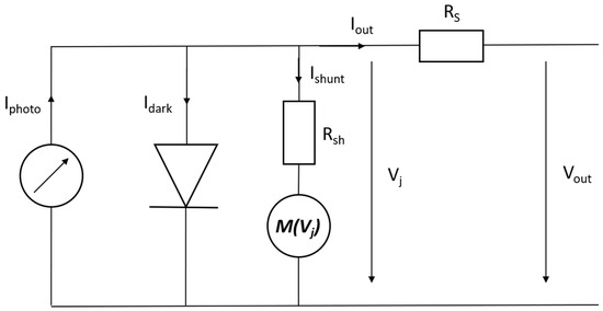
Figure 5.
Equivalent circuit diagram of a PV cell in the single-diode model. This model has already been used by Bishop et al. [61].
Equation (15) implicitly defines the IV curve [61]. is the saturation current of the diode, is the elementary charge, is the diode ideality factor, and is the Boltzmann constant. The current over the shunt resistance can be calculated by Equation (16) according to Bishop [61]. is the breakdown voltage, is the fraction of ohmic current involved in avalanche breakdown, and is the breakdown exponent. The breakdown parameters are taken from [66]. The Bishop model is capable of calculating the IV curve for an individual cell and is capable of calculating the IV curve of any connection of various cells either in parallel or in series or both. In particular, electrical mismatch is considered for the case that one cell is shaded, soiled, or defective.
The single-diode parameters are not immediately known. They are calculated by the methods presented in [67]. A detailed comparison of different algorithms to calculate the parameters was performed by Restrepo-Cuestas in [66,68]. They depend, on the one hand, on the module’s characteristics that are stated in the data sheet, and on the other hand, they depend on the illumination of the cell. Additionally, a potential efficiency reduction due to aging and module-specific production-related deviations from the design efficiency are considered. The data sheet’s power and efficiency are adjusted such that the model results match the measurements for the power, voltage, and current for a calibration interval. The temperature effect on the model parameters was considered as given in the data sheet to obtain the expected power under standard test conditions (STC).
The electrical model takes an initial estimate of the NOCT, according to the data sheet, for the cell temperature and calculates a power . This power estimate is then divided by the cell area, giving the surface power density for the cell. The thermal model receives the surface power density as one of the parameters to predict the cell temperature . These better estimates of the cell temperatures are then fed back into the electrical model, as it might differ from the originally estimated temperature. In the tested datasets used in this work, both power and temperature predictions converge after three iterations. The power changes afterwards by less than 0.01 W per iteration and the temperature by less than 0.01 K. Figure 6 illustrates the interconnection of the electrical and thermal models.
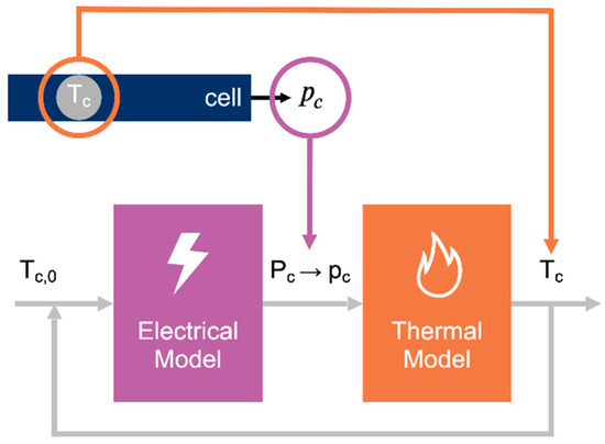
Figure 6.
Sketch describing the linkage between the electrical and thermal models, combining them to the electrothermal model.
The module is considered to be a serial connection of three sub-strings of 24 cells each. There is a bypass diode in parallel to each sub-string. The model allows assigning every cell its individual properties. In particular, every cell has its soiling transmittance. IV curves are calculated on cell, string, and module levels. Correspondingly, electrical mismatch losses are considered. The same current must flow through all cells unless the bypass diodes are active. The most affected cell limits the total current. If the total current is greater than the of the most affected cell, this cell dissipates energy. Also, the temperature of each cell is considered as input data. This cell-resolved temperature is used as an iterative input of the electrical and thermal model.
3.4. Non-Linear System of Equations
Equations (5)–(8) build a set of four equations with four unknown quantities. There are four unknown temperatures, , , , and . All other parameters are known (or estimated) as described in Table 1 and Table 2 above. Some of the temperatures occur in the fourth power. This makes the system non-linear and not analytically solvable. However, this system can be solved numerically. We used the fsolve function of the scipy package [69].
3.5. Thermal Inertia
As described above, the model solves a set of non-linear equations for the steady-state. In reality, the cell temperature does not instantly respond to a change in input parameters, e.g., a change in incoming radiation. The thermal inertia of the module is not considered when applying the steady-state assumption. To roughly consider the thermal inertia a rolling average is applied. Averaging is performed over ten temperature values modeled with the above described model and the average is assigned to the last of the corresponding timestamps of the final time series. The time interval is chosen as a simple best-by-test approach. In the following, the rolling average is applied to the developed model as well as to the models from the literature.
4. Experimental Validation and Discussion
4.1. Experiment with Clean PV Modules
The performance of the electrothermal model under clean conditions was analyzed within six consecutive days, from 26 April to 1 May 2023. In particular, the performance for module temperature determination was compared to measurements and the state-of-the-art models described in Section 2.1. The temperature was measured with a Pt-1000 sensor (uncertainty class B) which was mounted on the module’s rear side with an adhesive thermo-film. The module of interest is manufactured by JA Solar and has a nominal power of 390 W [48]. Details can be found in the data sheet [48]. All timestamps in this work refer to UTC + 1.
Figure 7 compares the modeled temperature to the measured one over the above-mentioned periods. In general, the model worked well and was capable of giving a good estimation of the module temperature. For some intervals, a negative bias was found (e.g., 26 April, 15:00–16:00) while the model overestimated the temperature for other time intervals (e.g., 1 May, 14:30–16:00). Reasons for this and possible solutions were assumed to be mostly related to the convection model. For example, currently, only the wind speed is considered, but not the wind direction. Also, the convection should in theory depend on the position of a given cell within the given module. The effects of the convection modeling will be discussed further related to the experiment with soiled modules (Section 4.2). Further potential enhancements could be a better consideration of thermal inertia which plays a particular role when the GTI or the wind speed suddenly changes.
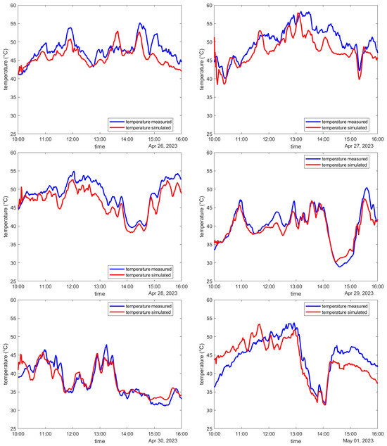
Figure 7.
Measured and simulated module temperatures of the clean module for the six-day long test period.
Three metrics were analyzed to describe the performance of the model. The root mean square error (RMSE), the mean average error (MAE), and the mean bias error (MBE) are described in Equation (17), where is the total number of data points, refers to the time stamp, is the measured value, and is the predicted value. is the average of all .
The obtained error metrics over the six days, 10:00 to 16:00 each, were an RMSE of 2.6 K, an MAE of 2.2 K, and an MBE of −1.3 K. The R2 value was 0.8677.
Figure 8 (left) shows the results of the developed model and the four above-mentioned thermal models from the literature for one exemplary day. On the right, this figure shows the two most important meteorological parameters impacting the module temperature, namely the irradiance (GTI) and the wind speed. Table 3 summarizes the error metrics of all thermal models. The developed model performed similarly to the two best models from the literature, the Faiman model and the NOCT model. The developed model had the lowest RMSE with a value of 2.6 K, which was marginally better than the next best Faiman model, while the MAE was insignificantly higher with a value of 2.2 K. The absolute value of the MBE of the developed model was 1.3 K and hence higher than the one of the NOCT model with a value of only 0.2 K. The temperature deviation had an impact on the module’s efficiency. Typically, the efficiency dropped by 0.4% for a temperature increase of 1 K. The impact of temperature deviation on the yield was not the decisive factor for our objective as the model was designed for hot-spot analysis. Quick hot-spot identification and hot-spot temperature estimation was possible with the new model and are discussed in the next section.
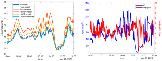
Figure 8.
(Left): Temperature determined with the different thermal models as well as the measured temperature as a function of time. Four models from the literature and the developed model are shown. An interval of the day April 29 has been chosen as an example. (Right): GTI and wind speed are shown for the exemplary time interval as these are key parameters influencing the module temperature.
Table 3.
Summary of the error metrics for the different thermal models, both from the literature and the developed model. This table refers to the clean state. The data refers to the entire test period consisting of six days.
4.2. Experiment with Soiled PV Modules
For the soiled experiment, one cell of the module was entirely covered with an artificial shading material, as shown also in Figure 2. The material used was a stack of foils and its transmissivity was roughly constant over the visible spectrum. The effective transmittance was 44.6% as determined by optical measurements and via analyzing the IV curves. The spectral transmittance is shown in Appendix A. The goal of the artificial soiling was to provoke a hot-spot and make the soiled cell dissipate power. Therefore, the qualitative regime of the transmittance is more important than its absolute value. Additionally, the hot-spot temperature and humidity can change the foils’ optical properties over time. The experiment was performed from 9 March to 14 March 2024.
Figure 9 compares the measured and simulated IV curves. For example, only four IV curves of one day, March 12, are shown with a time difference of 2 h each. One can see that the shapes of the IV curves are qualitatively correct. There is a slight tendency to predict too high open circuit voltages and too low short-circuit currents. The IV curve with the timestamp 14:00 was impacted the most. The reason was probably related to simplifications of the underlying electrical Bishop model [61]. The position of the maximum power point was calculated relatively accurately. The height of the plateau of the current differs slightly between measurement and simulation. The reason might be that the transmittance of the artificial soiling layer slightly changed over time. As the foils used as artificial soiling heated up, they might have changed their transmittance. Figure 10 compares the measured and simulated electrical powers in a plot as a function of time. In general, the electrical power was calculated well (RMSE = 2.1 W, MBE = −0.2 W, MAE = 1.6 W). The R2 of modeling the electrical power was 0.9991. On average, the relative deviation between the predicted and measured power was 1.37%. One subfigure corresponded to each day, starting in the upper left with the 9th of March and continuing to the 14th of March in the lower right.
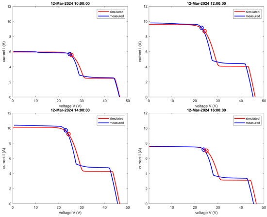
Figure 9.
Measured and simulated IV curves. Exemplary, one day and four timestamps are chosen (12 March 2024). Upper left 10:00, upper right 12:00, lower left 14:00, and lower right 16:00. The small circles indicate the maximum point points. The electrical simulation to calculate the IV curves was performed with the Bishop model [61].
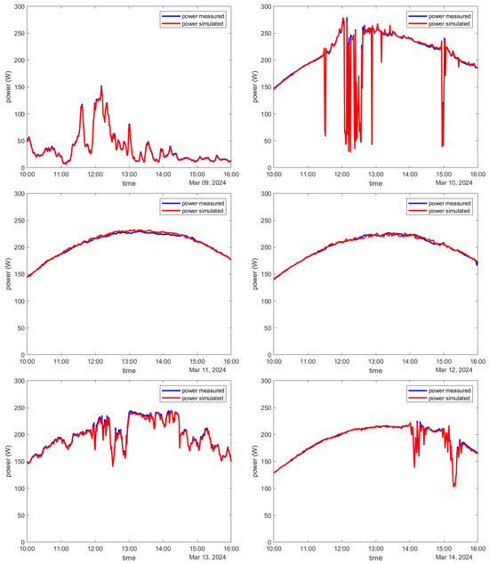
Figure 10.
Measured and simulated electrical powers for the entire time considered for the soiled experiment. Each subfigure shows the data for one day.
The right side of Figure 11 compares the measured and simulated hot-spot temperatures and the measured temperature of a clean cell. Each day is discussed individually. To explain and understand the features that occur one must have a look at the GTI, the wind speed, and the wind direction which are shown also in Figure 11, but on the left side each. On the 9 March, the temperature was simulated well with an RMSE of 4.8 K. This was a day with a low GTI and strong wind from the southwest direction. For the 10 March, the model predicted a hot-spot with temperatures about 20 K above those of the clean cells but underestimated the temperature significantly by more than 30 K resulting in an RMSE of 32.7 K and an MBE of −30.9 K. On that day, the GTI was generally pretty high and there was strong wind from the west direction. In this context, a high GTI referred to the GTI reaching about 1000 W/m2 at solar noon and, overall, only a few clouds over the day. On the 11 March, the temperature estimation was good for the first two hours of the analyzed time interval. Afterwards, the temperature was underestimated similarly to the 10 March resulting in an RMSE of 21 K and an MBE of −16.7 K. On the 11 March, the GTI was high and the wind from the west direction grew continuously stronger over the day. On the 12th the temperature was estimated well. In the morning the temperature was overestimated slightly while it is underestimated slightly in the afternoon, resulting in an RMSE of 12.5 K and an MBE of 1.5 K. In the morning there was basically no wind, and in the afternoon there was a slight wind coming from the west direction. The GTI was high. On the 13th the temperature was calculated overall accurately with an RMSE of 7.7 K and an MBE of 0.9 K. The GTI was high and there was a wind of about 5 m/s from the east direction. On the 14th of March, the temperature was, generally speaking, slightly underestimated with an RMSE of 11.2 K and an MBE of −6.6 K. The GTI was high and there was a small but continuously increasing wind from the west direction. Over six days, the model performed with an RMSE of 17.7 K, an MAE of 13.1 K, and an MBE of −9.0 K. The model achieved an R2 of 0.7712 and the hot-spot temperature increase compared with the clean cell was on average calculated with a deviation of 25.8%.
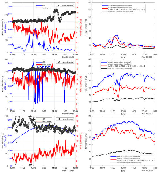
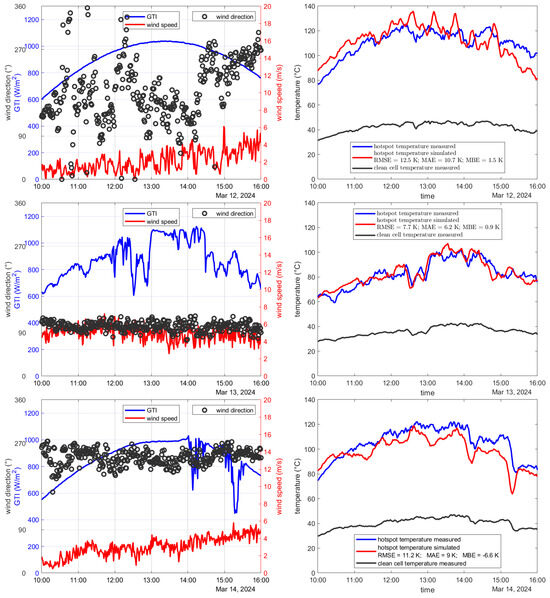
Figure 11.
The left subfigure of each column shows the most important meteorological data determining the temperature. The wind direction is given in degrees. Here, 0° corresponds to wind coming from the north direction. Then, it is counted clockwise. Meaning, e.g., 90° corresponds to wind coming from the east direction. The right subfigure of each column compares the measured and hot-spot temperatures simulated by the developed model. Additionally, the temperature of a clean cell, a non-hot-spot cell, is shown in dark gray. In total: RMSE = 17.7 K, MBE = −9.0 K, MAE = 13.1 K, R2 = 0.7712.
The deviations found are assumed to be mainly related to convection modeling. In the west of the PV testbench, there was a big hall that reduced the wind coming from that direction. The meteorological station measuring the wind was not affected by this hall for west winds. This means that in the case of the wind coming from the west direction, the wind speed was systematically overestimated for the convection modeling. This leads to an overestimation of the convection and an underestimation of the temperature. In particular, this explains the deviations for the 10th and 11th of March. For the 9th of March, there was a low GTI and therefore an overall low temperature. This also means that the effect of the convection was less pronounced. For the 12th and the 14th of March, there were overall only small wind speeds present. This caused the deviations to be lower. A more representative wind measurement would most likely improve the results significantly. At the same time, there will not be wind measurements in PV parks close to each PV module in the field. It is unlikely there will be accurate wind measurements for every location within a large PV park. Hence, the validation mimics a realistic situation and input data accuracy. Even with the observed deviations, the model is capable of distinguishing accurately between hot-spots and cells with a normal operation temperature.
5. Conclusions and Outlook
This paper has presented a new way of electrothermally modeling soiled PV modules. The electrical part of the model uses the established Bishop model. The model is capable of calculating the IV curves of a module, the electrical power output, and the module temperature with cell resolution. The calculated IV curves matched well with the measured ones and the power under regular operating conditions could be determined accurately (RMSE of the electrical power was 2.1 W and MBE was −0.2 K over 6 days and the nominal module power of 390 W). The average relative deviation between measured and simulated power was 1.37%. These metrics are an indication that the use of the single-diode model is unproblematic. However, replacing the single-diode model with the two-diode model is not expected to lead to significant improvements.
The meteorological parameters considered by the thermal model are the GTI measured by a reference cell, the wind speed, the infrared radiation measured by a pyrgeometer, the ambient temperature, and the air pressure. All meteorological data were measured at a weather station 100 m north of the testbench that contains the modules of interest. When calculating the temperature of a clean module, the model showed a similar performance to the two most accurate models, the Faiman model and the NOCT model, with only minor differences in the error metrics RMSE, MAE, and MBE, out of four well-established models.
The developed model was capable of calculating the hot-spot temperature of soiled or partially shaded modules. Over a test period of six days, the temperature estimation showed an RMSE of 17.7 K. At times the temperature prediction was accurate while it deviated for certain conditions. For the best individual day, the RMSE was as low as 4.8 K. The temperature increase caused by a hot-spot compared to a clean cell was determined on average with a relative deviation of 25.83%. The deviations have been explained and differences between the wind conditions directly next to the PV modules compared to the wind at the wind mast are assumed to be the main cause of the deviations. Such a spatial separation of the anemometer and the PV module is also to be expected in real PV plants, so the experimental setup is considered to be adequate.
The model manages to correctly predict whether the soiling or shading pattern is sufficient to cause a hot-spot. In case an IR image shows a hot-spot, the model is capable of stating if the hot-spot can be caused by soiling or shading or if it must be caused by a defect. Operators of a PV plant should be alarmed when either a hot-spot is detected on an IRT image or the developed electrothermal model states that a soiling pattern seen on an RGB image will cause a hot-spot. When both applies at the same time it is alarming as well. However, in this case cleaning is likely sufficient.
The results of this study suggest that the accuracy of the thermal model is limited by the uncertainty of the meteorological parameters used as an input. The electrical model is currently not limiting the thermal model. If a higher accuracy of the electrical model (better than the current 1.37% relative deviation) is desired, the underlying single-diode model could be replaced by the two-diode model.
The developed model can be used to enhance the monitoring of PV plants. The new method is applicable, for example, in combination with IR monitoring flights. It can potentially be applied to large scales.
Currently the method is only tested for technologies based on crystalline silicon. If the method was to be used for, e.g., thin-film or perovskite modules, larger deviation would be expected.
Further developments of the method can go in different directions. On the one hand, the method can be applied to different kinds of modules. In particular, it could be used for half-cell modules which are currently often used. On the other hand, improved convection models that consider also the wind direction could be implemented to enhance the model’s accuracy. Also, the developed model could be tested with image-based soiling information.
Author Contributions
Conceptualization, P.W., J.S. and S.W.; methodology, P.W., J.S. and S.W.; software, J.S. and P.W.; validation, P.W. and N.B.; formal analysis, P.W., J.S. and S.W.; data curation and data acquisition, J.S. and P.W.; writing—original draft preparation, P.W.; writing—review and editing, all; visualization, P.W. and J.S.; supervision, S.W., R.P.-P., M.R., F.S., M.d.C.A.-G., J.P., J.A.C. and A.F.; project administration, S.W.; funding acquisition, S.W. All authors have read and agreed to the published version of the manuscript.
Funding
This research was funded by the German Federal Ministry of Economic Affairs and Climate Action within the PVOptDigital project, grant number 03EE1107B.
Data Availability Statement
Data are available upon reasonable request. Data is not available publicly due to both privacy and legal reasons.
Conflicts of Interest
The authors declare no conflicts of interest.
Abbreviations
| PV | Photovoltaics |
| IRT, IR | Infrared thermography, Infrared |
| EL | Electroluminescence |
| RGB image | Red, Green, Blue image (image type) |
| IV curve | Current-voltage curve |
| UV light/radiation | Ultraviolet light/radiation |
| CNN | Convolutional Neural Network |
| STC | Standard test conditions |
| NOCT | Normal operating condition temperature |
| RMSE | Root mean square error |
| MAE | Mean average error |
| MBE | Mean bias error |
| Symbols | |
| Conductive heat transfer | |
| Convective heat transfer | |
| Specific heat capacity | |
| Electrical power | |
| Cell area | |
| Temperature | |
| Irradiance | |
| Wind speed | |
| Convective heat transfer coefficient | |
| Elementary charge | |
| Resistance | |
| Diode ideality factor | |
| Module efficiency | |
| Thermal radiation | |
| Thermal conductivity | |
| Hemispherical reflectance | |
| Absorptance | |
| Emissivity | |
| Hemispherical Transmittance | |
| Kinematic viscosity |
Appendix A
Figure A1 shows the optically measured spectral transmittance of the foils used as artificial soiling in blue. Averaging the spectral transmittance weighted by the solar spectrum shown in red (ISO9845-1 Main Spectra GTI) and the spectral response of the module shown in dark gray [70,71] results in a wavelength averaged transmittance of 44.6%.

Figure A1.
In blue, spectral transmittance against wavelength of the used artificial soiling. In red, solar spectrum used for averaging the spectral transmittance. In dark gray, spectral response of a mono-Si solar cell. Weighted averaging results in an effective transmittance of 44.6%.
Figure A1.
In blue, spectral transmittance against wavelength of the used artificial soiling. In red, solar spectrum used for averaging the spectral transmittance. In dark gray, spectral response of a mono-Si solar cell. Weighted averaging results in an effective transmittance of 44.6%.

Appendix B
The simulation parameters are shown in Table A1. Note that the single-diode parameter cannot be stated here as the parameters vary with the meteorological conditions, in particular the current source depends on the incoming irradiance.
Figure A2 shows the setup from the top. Figure 2 has previously shown the setup including the artificial soiling material.
Table A1.
Summary of the simulation parameters. Breakdown parameters are taken from [66,68]. The parameters are corrected for aging.
Table A1.
Summary of the simulation parameters. Breakdown parameters are taken from [66,68]. The parameters are corrected for aging.
| Quantity | Value |
|---|---|
| Breakdown factor | 0.002 |
| Breakdown voltage | −14 V |
| Trigger voltage of the bypass diode | −0.5 |
| Breakdown exponential factor | 3 |
| Efficiency | 0.17622% |
| Short circuit current under STC | 9.61 A |
| Open circuit voltage under STC | 47.13 V |
| Power under STC | 349 W |
| MPP current under STC | 9.26 A |
| MPP voltage under STC | 37.80 V |
| Temperature coefficient of the power | −0.37 %/K |

Figure A2.
Top view of the setup used. The lower fifth module from the right is used for the experiments. Figure 2 has already shown the module with its artificial shading.
Figure A2.
Top view of the setup used. The lower fifth module from the right is used for the experiments. Figure 2 has already shown the module with its artificial shading.

References
- Bouckaert, S.; Pales, A.F.; McGlade, C.; Remme, U.; Wanner, B.; Varro, L.; D’Ambrosio, D.; Spencer, T. Net Zero by 2050: A Roadmap for the Global Energy Sector; The National Academies of Sciences, Engineering, and Medicine: Washington, DC, USA, 2021; p. 224. [Google Scholar]
- Gielen, D.; Gorini, R.; Wagner, N.; Leme, R.; Gutierrez, L.; Prakash, G.; Asmelash, E.; Janeiro, L.; Gallina, G.; Vale, G. Global Energy Transformation: A Roadmap to 2050; International Renewable Energy Agency (IRENA): Masdar City, United Arab Emirates, 2019; p. 52. [Google Scholar]
- Honrubia-Escribano, A.; Ramirez, F.J.; Gómez-Lázaro, E.; Garcia-Villaverde, P.M.; Ruiz-Ortega, M.J.; Parra-Requena, G. Influence of solar technology in the economic performance of PV power plants in Europe. A comprehensive analysis. Renew. Sustain. Energy Rev. 2018, 82, 488–501. [Google Scholar] [CrossRef]
- Deitsch, S.; Christlein, V.; Berger, S.; Buerhop-Lutz, C.; Maier, A.; Gallwitz, F.; Riess, C. Automatic classification of defective photovoltaic module cells in electroluminescence images. Sol. Energy 2019, 185, 455–468. [Google Scholar] [CrossRef]
- Köntges, M.; Kurtz, S.; Packard, C.; Jahn, U.; Berger, K.A.; Kato, K.; Friesen, T.; Liu, H.; Van Iseghem, M.; Wohlgemuth, J. Review of Failures of Photovoltaic Modules; Istituto Sostenibilità Applicata All’ambiente Costruito: Mendrisio, Switzerland, 2014. [Google Scholar]
- IEC 61215(04); Crystalline Silicon Terrestrial Photovoltaic (PV) Modules—Design Qualification and Type Approval. International Standard IEC: Geneva, Switzerland, 2005.
- Polo, J.; Martín-Chivelet, N.; Sanz-Saiz, C.; Alonso-Montesinos, J.; López, G.; Alonso-Abella, M.; Battles, F.J.; Marzo, A.; Hanrieder, N. Modeling soiling losses for rooftop PV systems in suburban areas with nearby forest in Madrid. Renew. Energy 2021, 178, 420–428. [Google Scholar] [CrossRef]
- Smestad, G.P.; Germer, T.A.; Alrashidi, H.; Fernández, E.F.; Dey, S.; Brahma, H.; Sarmah, N.; Ghosh, A.; Sellami, N.; Hassan, I.A. Modelling photovoltaic soiling losses through optical characterization. Sci. Rep. 2020, 10, 58. [Google Scholar] [CrossRef] [PubMed]
- Shen, Y.; Xu, Z.; Wang, Y.; Li, C.; Zhang, J.; Zhang, K.; Wei, H. Temperature Estimation of Partially Shaded Photovoltaic Modules Using a Multiphysics Model. IEEE J. Photovolt. 2022, 12, 1243–1251. [Google Scholar] [CrossRef]
- Pavan, A.M.; Mellit, A.; De Pieri, D. The effect of soiling on energy production for large-scale photovoltaic plants. Sol. Energy 2011, 85, 1128–1136. [Google Scholar] [CrossRef]
- Ilse, K.; Micheli, L.; Figgis, B.W.; Lange, K.; Daßler, D.; Hanifi, H.; Wolfertstetter, F.; Naumann, V.; Hagendorf, C.; Gottschalg, R. Techno-economic assessment of soiling losses and mitigation strategies for solar power generation. Joule 2019, 3, 2303–2321. [Google Scholar] [CrossRef]
- Maghami, M.R.; Hizam, H.; Gomes, C.; Radzi, M.A.; Rezadad, M.I.; Hajighorbani, S. Power loss due to soiling on solar panel: A review. Renew. Sustain. Energy Rev. 2016, 59, 1307–1316. [Google Scholar] [CrossRef]
- Lamaamar, I.; Tilioua, A.; Zaid, Z.B.; Babaoui, A.; Ettakni, M.; Alaoui, M.A.H. Evaluation of different models for validating of photovoltaic cell temperature under semi-arid conditions. Heliyon 2021, 7, e08534. [Google Scholar] [CrossRef]
- Vumbugwa, M.; Crozier McCleland, J.; Van Dyk, E.; Vorster, F.; Serameng, T. Effects of current mismatch due to uneven soiling on the performance of multi-crystalline silicon module strings. J. Energy S. Afr. 2020, 31, 62–72. [Google Scholar] [CrossRef]
- Winkel, P.; Wilbert, S.; Röger, M.; Krauth, J.J.; Algner, N.; Nouri, B.; Wolfertstetter, F.; Carballo, J.A.; Alonso-Garcia, M.C.; Polo, J. Cell-Resolved PV Soiling Measurement Using Drone Images. Remote Sens. 2024, 16, 2617. [Google Scholar] [CrossRef]
- Qasem, H.; Mnatsakanyan, A.; Banda, P. Assessing dust on PV modules using image processing techniques. In Proceedings of the 2016 IEEE 43rd Photovoltaic Specialists Conference (PVSC), Portland, OR, USA, 5–10 June 2016. [Google Scholar]
- Hwang, P.C.; Ku, C.C.-Y.; Chan, J.C.-C. Soiling detection for photovoltaic modules based on an intelligent method with image processing. In Proceedings of the 2020 IEEE International Conference on Consumer Electronics-Taiwan (ICCE-Taiwan), Taoyuan, Taiwan, 28–30 September 2020. [Google Scholar]
- Li, X.; Yang, Q.; Chen, Z.; Luo, X.; Yan, W. Visible defects detection based on UAV-based inspection in large-scale photovoltaic systems. IET Renew. Power Gener. 2017, 11, 1234–1244. [Google Scholar] [CrossRef]
- Cipriani, G.; D’Amico, A.; Guarino, S.; Manno, D.; Traverso, M.; Di Dio, V. Convolutional neural network for dust and hotspot classification in PV modules. Energies 2020, 13, 6357. [Google Scholar] [CrossRef]
- De Soto, W.; Klein, S.A.; Beckman, W.A. Improvement and validation of a model for photovoltaic array performance. Sol. Energy 2006, 80, 78–88. [Google Scholar] [CrossRef]
- Touati, F.; Chowdhury, N.A.; Benhmed, K.; Gonzales, A.J.S.P.; Al-Hitmi, M.A.; Benammar, M.; Gastli, A.; Ben-Brahim, L. Long-term performance analysis and power prediction of PV technology in the State of Qatar. Renew. Energy 2017, 113, 952–965. [Google Scholar] [CrossRef]
- Busquet, S.; Kobayashi, J. Modelling daily PV performance as a function of irradiation, ambient temperature, soiling, wind speed, and aging-Applied to PV modules operating in Maui. In Proceedings of the 2018 IEEE 7th World Conference on Photovoltaic Energy Conversion (WCPEC) (A Joint Conference of 45th IEEE PVSC, 28th PVSEC & 34th EU PVSEC), Waikoloa, HI, USA, 10–15 June 2018. [Google Scholar]
- Mittag, M.; Vogt, L.; Herzog, C.; Neuhaus, H. Thermal modelling of photovoltaic modules in operation and production. In Proceedings of the 36th European Photovoltaic Solar Energy Conference and Exhibition (EUPVSEC), Marseille, France, 9–13 September 2019. [Google Scholar]
- Tuncel, B.; Ozden, T.; Balog, R.; Akinoglu, B. Dynamic thermal modelling of PV performance and effect of heat capacity on the module temperature. Case Stud. Therm. Eng. 2020, 22, 100754. [Google Scholar] [CrossRef]
- Olukan, T.A.; Emziane, M. A comparative analysis of PV module temperature models. Energy Procedia 2014, 62, 694–703. [Google Scholar] [CrossRef]
- Ross, R. Design techniques for flat-plate photovoltaic arrays. In Proceedings of the 15th Photovoltaic Specialists Conference, Orlando, FL, USA, 12–15 May 1981. [Google Scholar]
- King, D.L.; Kratochvil, J.A.; Boyson, W.E. Photovoltaic Array Performance Model; Citeseer: University Park, PA, USA, 2004; Volume 8. [Google Scholar]
- Faiman, D. Assessing the outdoor operating temperature of photovoltaic modules. Prog. Photovolt. Res. Appl. 2008, 16, 307–315. [Google Scholar] [CrossRef]
- Gilman, P. SAM Photovoltaic Model Technical Reference; National Renewable Energy Lab. (NREL): Golden, CO, USA, 2015. [Google Scholar]
- Skoplaki, E.; Palyvos, J.A. Operating temperature of photovoltaic modules: A survey of pertinent correlations. Renew. Energy 2009, 34, 23–29. [Google Scholar] [CrossRef]
- Qian, J.; Thomson, A.; Blakers, A.; Ernst, M. Comparison of half-cell and full-cell module hotspot-induced temperature by simulation. IEEE J. Photovolt. 2018, 8, 834–839. [Google Scholar] [CrossRef]
- Solheim, H.J.; Fjær, H.G.; Sørheim, E.A.; Foss, S.E. Measurement and simulation of hot spots in solar cells. Energy Procedia 2013, 38, 183–189. [Google Scholar] [CrossRef][Green Version]
- Rossi, D.; Omaña, M.; Giaffreda, D.; Metra, C. Modeling and detection of hotspot in shaded photovoltaic cells. IEEE Trans. Very Large Scale Integr. (VLSI) Syst. 2014, 23, 1031–1039. [Google Scholar] [CrossRef]
- Geisemeyer, I.; Fertig, F.; Warta, W.; Rein, S.; Schubert, M. Prediction of silicon PV module temperature for hot spots and worst case partial shading situations using spatially resolved lock-in thermography. Sol. Energy Mater. Sol. Cells 2014, 120, 259–269. [Google Scholar] [CrossRef]
- Winkel, P.; Wilbert, S.; Wolfertstetter, F.; Röger, M.; Krauth, J.J.; Algner, N.; Zarzalejo, L.; Martinez, D.; Polo, J.; Alsonso García, M.C.; et al. Zell-aufgelöste Bestimmung der Verschmutzung von PVModulen mit bildgebenden Verfahren. In Proceedings of the PV Symposium, Freiburg im Breisgau, Germany, 21–23 June 2022. [Google Scholar]
- Tool, C.; Burgers, A.; Manshanden, P.; Weeber, A.; Van Straaten, B. Influence of wafer thickness on the performance of multicrystalline Si solar cells: An experimental study. Prog. Photovolt. Res. Appl. 2002, 10, 279–291. [Google Scholar] [CrossRef]
- Lorenz, A.; Münzer, A.; Lehner, M.; Greutmann, R.; Brocker, H.; Reinecke, H.; Clement, F. High-throughput front and rear side metallization of silicon solar cells using rotary screen printing. Energy Procedia 2017, 124, 680–690. [Google Scholar] [CrossRef]
- Zheng, D.; Hunt, E.R., Jr.; Running, S.W. A daily soil temperature model based on air temperature and precipitation for continental applications. Clim. Res. 1993, 2, 183–191. [Google Scholar] [CrossRef]
- Xu, C.; Qu, J.J.; Hao, X.; Zhu, Z.; Gutenberg, L. Surface soil temperature seasonal variation estimation in a forested area using combined satellite observations and in-situ measurements. Int. J. Appl. Earth Obs. Geoinf. 2020, 91, 102156. [Google Scholar] [CrossRef]
- Araghi, A.; Mousavi-Baygi, M.; Adamowski, J.; Martinez, C.; van der Ploeg, M. Forecasting soil temperature based on surface air temperature using a wavelet artificial neural network. Meteorol. Appl. 2017, 24, 603–611. [Google Scholar] [CrossRef]
- Zhou, J.; Yi, Q.; Wang, Y.; Ye, Z. Temperature distribution of photovoltaic module based on finite element simulation. Sol. Energy 2015, 111, 97–103. [Google Scholar] [CrossRef]
- Pfreundt, A.; Yucebas, D.; Beinert, A.; Verissimo Mesquita, L.; Pitta Bauermann, L.; Romer, P.; Mittag, M. Post-processing thickness variation of PV module materials and its impact on temperature, mechanical stress and power. In Proceedings of the 36th EU PV Solar Energy Conference and Exhibition, Marseille, France, 9–13 September 2019. [Google Scholar]
- Hoang, P.; Bourdin, V.; Liu, Q.; Caruso, G.; Archambault, V. Coupling optical and thermal models to accurately predict PV panel electricity production. Sol. Energy Mater. Sol. Cells 2014, 125, 325–338. [Google Scholar] [CrossRef]
- Priyadarshini, B.G.; Sharma, A.K. Design of multi-layer anti-reflection coating for terrestrial solar panel glass. Bull. Mater. Sci. 2016, 39, 683–689. [Google Scholar] [CrossRef]
- Notton, G.; Cristofari, C.; Mattei, M.; Poggi, P. Modelling of a double-glass photovoltaic module using finite differences. Appl. Therm. Eng. 2005, 25, 2854–2877. [Google Scholar] [CrossRef]
- Lee, B.; Liu, J.; Sun, B.; Shen, C.; Dai, G. Thermally conductive and electrically insulating EVA composite encapsulants for solar photovoltaic (PV) cell. Express Polym. Lett. 2008, 2, 357–363. [Google Scholar] [CrossRef]
- Wolf, A.; Pohl, P.; Brendel, R. Determination of thermophysical properties of thin films for photovoltaic applications. In Proceedings of the Conference Record of the Thirty-first IEEE Photovoltaic Specialists Conference, Lake Buena Vista, FL, USA, 3–7 January 2005. [Google Scholar]
- Solar, J. 395W PERC Module, J.S. 375-395/PR, Editor. 2024.
- United States Committee on Extension to the Standard Atmosphere. US Standard Atmosphere, 1976; National Oceanic and Amospheric [sic] Administration: Washington, DC, USA, 1976. [Google Scholar]
- Siebers, D.L. Experimental Mixed Convection Heat Transfer from a Large, Vertical Surface in a Horizontal Flow; Stanford University: Stanford, CA, USA, 1983. [Google Scholar]
- Kreith, F.; Kreider, J.F. Principles of Solar Engineering; McGraw-Hill: New York, NY, USA, 1978. [Google Scholar]
- Cole, R.; Sturrock, N. The convective heat exchange at the external surface of buildings. Build. Environ. 1977, 12, 207–214. [Google Scholar] [CrossRef]
- Bell, C. Fluid Dynamics Component of Chemical Engineering Design Library (ChEDL). 2023. Available online: https://github.com/CalebBell/fluids (accessed on 1 March 2023).
- Ilse, K.K.; Figgis, B.W.; Naumann, V.; Hagendorf, C.; Bagdahn, J. Fundamentals of soiling processes on photovoltaic modules. Renew. Sustain. Energy Rev. 2018, 98, 239–254. [Google Scholar] [CrossRef]
- Devi, A.; Satheesh, S.K. Global maps of aerosol single scattering albedo using combined CERES-MODIS retrieval. Atmos. Chem. Phys. 2022, 22, 5365–5376. [Google Scholar] [CrossRef]
- Rubio, E.; Caselles, V.; Badenas, C. Emissivity measurements of several soils and vegetation types in the 8–14 μm Wave band: Analysis of two field methods. Remote Sens. Environ. 1997, 59, 490–521. [Google Scholar] [CrossRef]
- Hamdhan, I.N.; Clarke, B.G. Determination of thermal conductivity of coarse and fine sand soils. In Proceedings of the World Geothermal Congress, Bali, Indonesia, 25–29 April 2010. [Google Scholar]
- The Engineering ToolBox. Surface Emissivity Coefficients. 2003. Available online: https://www.engineeringtoolbox.com/emissivity-coefficients-d_447.html (accessed on 14 June 2024).
- The Engineering ToolBox. Plastics—Thermal Conductivity Coefficients. 2011. Available online: https://www.engineeringtoolbox.com/thermal-conductivity-plastics-d_1786.html (accessed on 14 June 2024).
- Sutha, S.; Suresh, S.; Raj, B.; Ravi, K. Transparent alumina based superhydrophobic self–cleaning coatings for solar cell cover glass applications. Sol. Energy Mater. Sol. Cells 2017, 165, 128–137. [Google Scholar] [CrossRef]
- Bishop, J. Computer simulation of the effects of electrical mismatches in photovoltaic cell interconnection circuits. Sol. Cells 1988, 25, 73–89. [Google Scholar] [CrossRef]
- Post, D.; Fimbres, A.; Matthias, A.; Sano, E.; Accioly, L.; Batchily, A.; Ferreira, L. Predicting soil albedo from soil color and spectral reflectance data. Soil Sci. Soc. Am. J. 2000, 64, 1027–1034. [Google Scholar] [CrossRef]
- Enriquez, R.; Zarzalejo, L.; Jiménez, M.; Heras, M. Ground reflectance estimation by means of horizontal and vertical radiation measurements. Sol. Energy 2012, 86, 3216–3226. [Google Scholar] [CrossRef]
- Holmgren, W.F.; Andrews, R.W.; Lorenzo, A.T.; Stein, J.S. PVLIB python 2015. In Proceedings of the 2015 IEEE 42nd Photovoltaic Specialist Conference (PVSC), New Orleans, LA, USA, 14–19 June 2015. [Google Scholar]
- Holmgren, W.F.; Hansen, C.W.; Mikofski, M.A. pvlib python: A python package for modeling solar energy systems. J. Open Source Softw. 2018, 3, 884. [Google Scholar] [CrossRef]
- Restrepo-Cuestas, B.J.; Montano, J.; Ramos-Paja, C.A.; Trejos-Grisales, L.A.; Orozco-Gutierrez, M.L. Parameter estimation of the bishop photovoltaic model using a genetic algorithm. Appl. Sci. 2022, 12, 2927. [Google Scholar] [CrossRef]
- Dobos, A.P. An Improved Coefficient Calculator for the California Energy Commission 6 Parameter Photovoltaic Module Model; National Renewable Energy Lab. (NREL): Golden, CO, USA, 2012. [Google Scholar]
- Restrepo-Cuestas, B.J.; Montano, J. Bishop model parameter estimation in photovoltaic cells using metaheuristic optimization techniques. Sol. Energy 2024, 270, 112410. [Google Scholar] [CrossRef]
- The SciPy Community. scipy.optimize.fsolve. 2014. Available online: https://docs.scipy.org/doc/scipy/reference/generated/scipy.optimize.fsolve.html (accessed on 29 July 2014).
- Jessen, W.; Wilbert, S.; Gueymard, C.A.; Polo, J.; Bian, Z.; Driesse, A.; Habte, A.; Marzo, A.; Armstrong, P.R.; Vignola, F. Proposal and evaluation of subordinate standard solar irradiance spectra for applications in solar energy systems. Sol. Energy 2018, 168, 30–43. [Google Scholar] [CrossRef]
- Winter, S.; Friedrich, D.; Sperling, A. Effects of the new standard IEC 60904-3: 2008 on the calibration results of common solar cell types. In Proceedings of the 24th European Photovoltaic Solar Energy Conference, Hamburg, Germany, 21–25 September 2009. [Google Scholar]


Disclaimer/Publisher’s Note: The statements, opinions and data contained in all publications are solely those of the individual author(s) and contributor(s) and not of MDPI and/or the editor(s). MDPI and/or the editor(s) disclaim responsibility for any injury to people or property resulting from any ideas, methods, instructions or products referred to in the content. |
© 2024 by the authors. Licensee MDPI, Basel, Switzerland. This article is an open access article distributed under the terms and conditions of the Creative Commons Attribution (CC BY) license (https://creativecommons.org/licenses/by/4.0/).