Abstract
The McMaster nuclear reactor (MNR) is an important research facility that not only provides researchers with neutrons for fundamental science, but also supplies the medical industry with isotopes used for cancer treatment. To ensure the safety and performance of the MNR, modeling of the thermal hydraulics during nominal and accidental conditions is required. For such a task, system codes are customarily used. While system codes can assess the safety aspects of complex thermal–hydraulic systems, the question arises whether such systems can be modeled appropriately in a three-dimensional manner, such as computation fluid dynamics (CFD), while capturing the thermal mixing of the coolant. Modeling the thermal hydraulics of nuclear research reactors using CFD is relatively new. Therefore, validating such methods against experimental data is of utmost importance. The validation of CFD is the main focus of this work. More specifically, the influence of the loss of heat sink on the pool temperature is assessed using the CFD code Ansys CFX. The validation basis was provided by an experiment performed at the MNR in March 2023. In this experiment, the secondary heat removal system was intentionally shut down, and the pool temperature was measured in a few positions. The results obtained by modeling the loss of heat sink in the MNR using Ansys CFX agree well with the experiment.
1. Introduction
Many countries consider nuclear technologies as a key to getting to ‘net-zero’ and to the future of science, technology, and medicine. Not only is the production of electricity and heat from nuclear power plants important and critical, but there is also an equal and growing need to produce radioisotopes for cutting-edge cancer therapy, to develop and test new materials, etc. With the expected increase of new nuclear deployments, it is also very desirable to improve analysis methods for nuclear reactors. However, the introduction of new codes or methods requires extensive experimental studies for validation purposes. As it is typically challenging to conduct experiments with a nuclear reactor, today’s analyses are mainly based on extensive coupled modeling of neutronics and thermal hydraulics during nominal operation, as well as in accidental scenarios. For the assessment of entire facilities, so-called system codes like RELAP [1] and CATHARE [2] are used to model extensive thermal–hydraulic systems and to provide safety-related information. Although these codes can accommodate the safety needs of nuclear reactors, a compelling train of thought leads to the appropriateness of using computational fluid dynamics (CFD) for a three-dimensional and more realistic assessment of specific areas/components of interest in the reactor. CFD code-to-experiment validation is already being used in many non-nuclear-related applications [3,4]. Although not a fully new approach, CFD can provide more details and, therefore, a better understanding of complex phenomena in nuclear reactors. Hence, a broader use of CFD for reactor analyses is desirable. To exploit its full potential for nuclear reactor applications, CFD must be validated using experimental data from different reactor types and various thermal–hydraulic regimes [5].
For this purpose, but also to characterize the primary circuit as a thermal system, an experiment was performed in March 2023 at the McMaster nuclear reactor (MNR), a research reactor capable of conducting experiments within the reactor core itself. The experiment initially aimed to measure the temperature feedback coefficient due to an increasing pool temperature in the framework of the IAEA coordinated research project (CRP) “Development of neutronic and thermal-hydraulic coupled calculational methodologies for research reactors including treatment of uncertainties” [6]. To do this, the reactor was operated at full power without the secondary coolant pumps being turned on. This was possible until the pool temperature reached the maximum allowed, as stated in the safety operations envelope [7]. As the core and pool were very well instrumented for this experiment, other phenomena could be measured, too. Here, the mixing of the coolant with different temperatures inside the pool was investigated. With thermocouples in different positions, the mixing was experimentally measured. These results are compared with CFD simulations using Ansys CFX [8].
2. McMaster Nuclear Reactor (MNR)
The McMaster nuclear reactor (MNR) is Canada’s most powerful research reactor, located in and operated by McMaster University in Hamilton, Ontario [9]. It was built in the 1950s and achieved its first criticality in 1959. Today, the MNR is one of the world’s leading facilities for the production of medical radioisotopes, especially iodine 125. The neutrons obtained from the MNR’s beam tubes are currently utilized for various purposes, such as neutron radiography and neutron diffraction experiments. The MNR is a pool-type material test reactor cooled and moderated by light water. The reactor consists of six control elements (a control element is a fuel element that contains a control rod in addition to nine fuel plates) and around 30 standard fuel elements (a standard fuel element contains 18 fuel plates, of which 16 are actually fuel plates and 2 are dummy plates) in a typical core loading. The control fuel elements house control rods, of which five are made of Ag-In-Cd and are used for macroscopic reactivity control, while the sixth is used for automatic control and is made of stainless steel. There are multiple positions for material irradiation inside the reactor core.
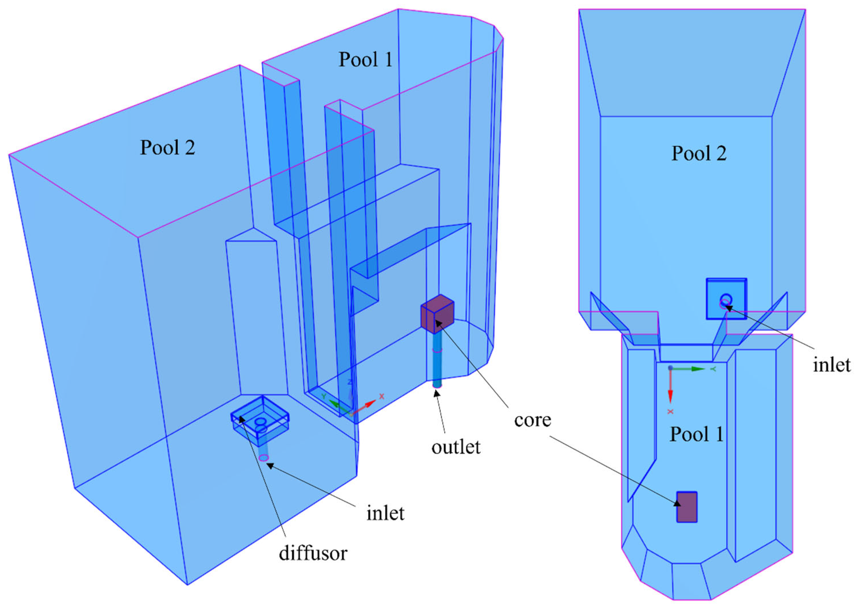
Currently, the reactor operates with a thermal power of 3 MW on a 24/5 schedule, with a power upgrade to 5 MW in planning. In the long run, even a 24/7 operation is considered to significantly boost the output of radioisotopes. A U3Si2 dispersion fuel with an enrichment of 19.75% is used. The reactor pool consists of two adjacent parts: pool 1 and pool 2 (see Figure 1). The reactor core and beam tube installations for scientific experiments are located in pool 1. The diffusor from which the coolant water reenters the pool is located in pool 2. Additionally, pool 2 offers housing for irradiated components and storage for spent fuel. A 10-m-high reinforced concrete structure provides structural integrity and biological shielding. In this CAD model created by using SolidWorks 2023, as explained in Section 3, the core itself is reduced to a red cuboid, for which water is assigned as a material. In reality, the MNR core consists of a 9 × 6 grid that contains 32 fuel assemblies, 7 graphite reflector assemblies, 6 control fuel assemblies, 1 beryllium reflector assembly, and 8 empty water sites. A typical fuel assembly is shown in Figure 2. A side view is shown in Figure 2a, while a top view, showing each fuel plate, is shown in Figure 2b.

Figure 1.
CAD model of the MNR pool. The core is denoted by the red cuboid. The pool’s inlet and outlet are both shown. The concrete housing is not shown in this figure.
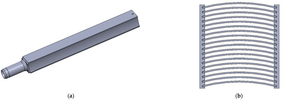
Figure 2.
(a) shows the side view of one of the MNR fuel assemblies, while (b) shows the top view.
3. Pool Temperature Experiment
In March 2023, an experiment was conducted at the MNR to measure pool temperature feedback within the framework of an IAEA CRP [6]. To accomplish this, the MNR’s secondary heat removal system was intentionally deactivated while the reactor was running at its full power of 3 MW, thus increasing the temperature of the primary system and the pool. From a reactor physics point of view, an increase in pool temperature implies a decrease in reactivity due to the negative temperature feedback coefficient of the light water-moderated MNR. Therefore, to maintain constant power throughout the experiment, the regulating rod was automatically retracted with increasing pool temperature, providing the possibility of measuring the reactivity coefficient.
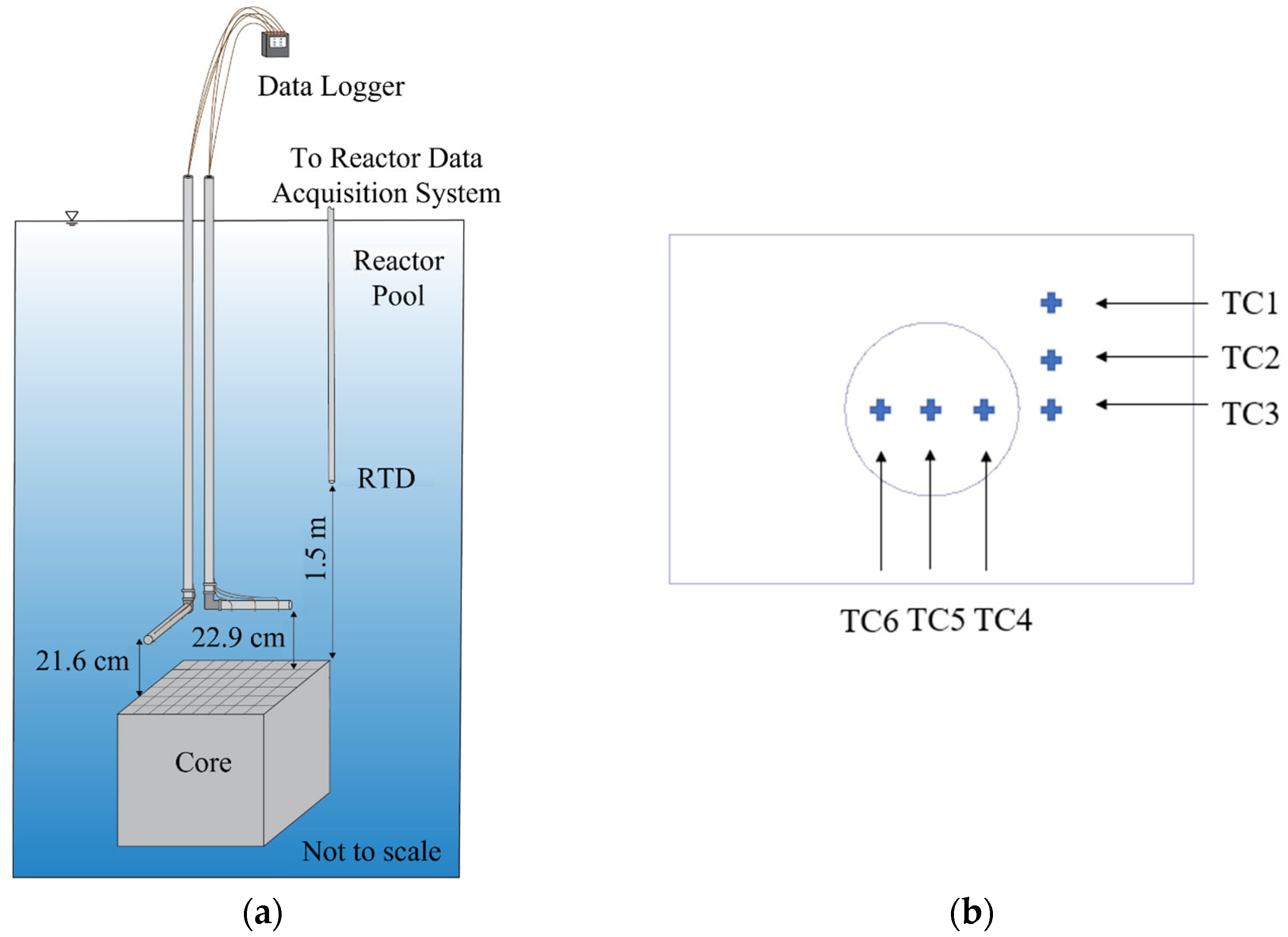
In addition to the resistance temperature detector (RTD), which is used in the reactor control system, a special structure that holds six thermocouples was placed right above the core to obtain a higher resolution of the temperature measurements (see Figure 3).

Figure 3.
(a) shows the thermocouple rake, while (b) shows the thermocouple holders.
Two heating/cooling cycles/transients took place in this experiment. The experiments started with a precooled pool with a minimum temperature of approximately 18 °C. In each cycle, the secondary coolant pumps were turned off, and the pool temperature increased to about 38 °C. At this point, the secondary pumps were cranked back to full power, leading to a temperature decline back to 18 °C. This fast change of the coolant temperature at the pool inlet led to stratification, including a buildup of thermal layers, which could be captured by the installed thermocouples and the RTD (see Figure 3).
4. Flow Equations and Numerical Models
The flow equations encompass a statement of the laws of the conservation of mass, momentum, and energy. The conservation of mass is expressed as:
The conservation of momentum is expressed as:
The conservation of momentum is expressed as:
The experimental sequence was modeled using Ansys CFX 2024.R1, a CFD code part of the Ansys suite [6]. CFX is a vertex-based finite volume code capable of modeling different liquid flows, such as laminar and turbulent flows. Many turbulence models are available in CFX. The turbulence in this work was treated using a Reynolds-averaged Navier–Stokes (RANS) approach [10].
The coolant flow was expected to be turbulent in the vicinity of the pool inlet due to the high mass flow and relatively thin pipe, while in the pool, the flow is rather laminar. Despite these drastic changes in flow behavior, the SST turbulence model was chosen since it is able to model the near-wall region quite well, which is important for the region in the vicinity of the inlet. The laminar flow at the walls of the pool is not of high interest for this work, since the pool containing material was not modeled, so that no heat transfer would occur at the wall. Additionally, the SST model is an industry standard [11,12] and its robustness has been proven in previous work [13].
5. Modeling Approach
The CAD model of the MNR pool (see Figure 1) was built in SolidWorks [10] based on technical drawings. The general model contains the two pools and the core. Based on the goal of this transient, the CAD model was simplified assuming the following points:
- The pool installations are omitted. This assumption is expected to lead to somewhat different flow patterns compared to reality, since the water flows from the inlet, into the pool, and then to the outlet of the reactor. Thus, the CFD simulations are expected to show simplified flow patterns, including less mixing than in reality.
- The width of the gate that separates the two pools is assumed to be constant while preserving the flow area of the real one. In reality, the gate is broader at the top than at the bottom.
- Due to the nature of the transient and its long duration, the reactor core is not modeled explicitly to save computational resources (see Section 2). This also implies that no heat is deposited in the core. The heat deposited in the pool is taken into account by the inlet temperature boundary condition, which follows the outlet temperature of the heat exchanger.
- The concrete containment of the pool is not taken into account in the transient, as it is assumed to play a negligible role in this experiment [14].
Due to the simplified modeling approach of the core, the results presented here only strengthen the case for the use of CFD to correctly capture fluid mixing and turbulence in the most common industrial approach (RANS). However, it cannot be used to push forward the validation of CFD for heat transfer within the reactor core, as, in these simulations, the heat was set as a boundary condition in the coolant inlet following the measured profile.
5.1. Mesh
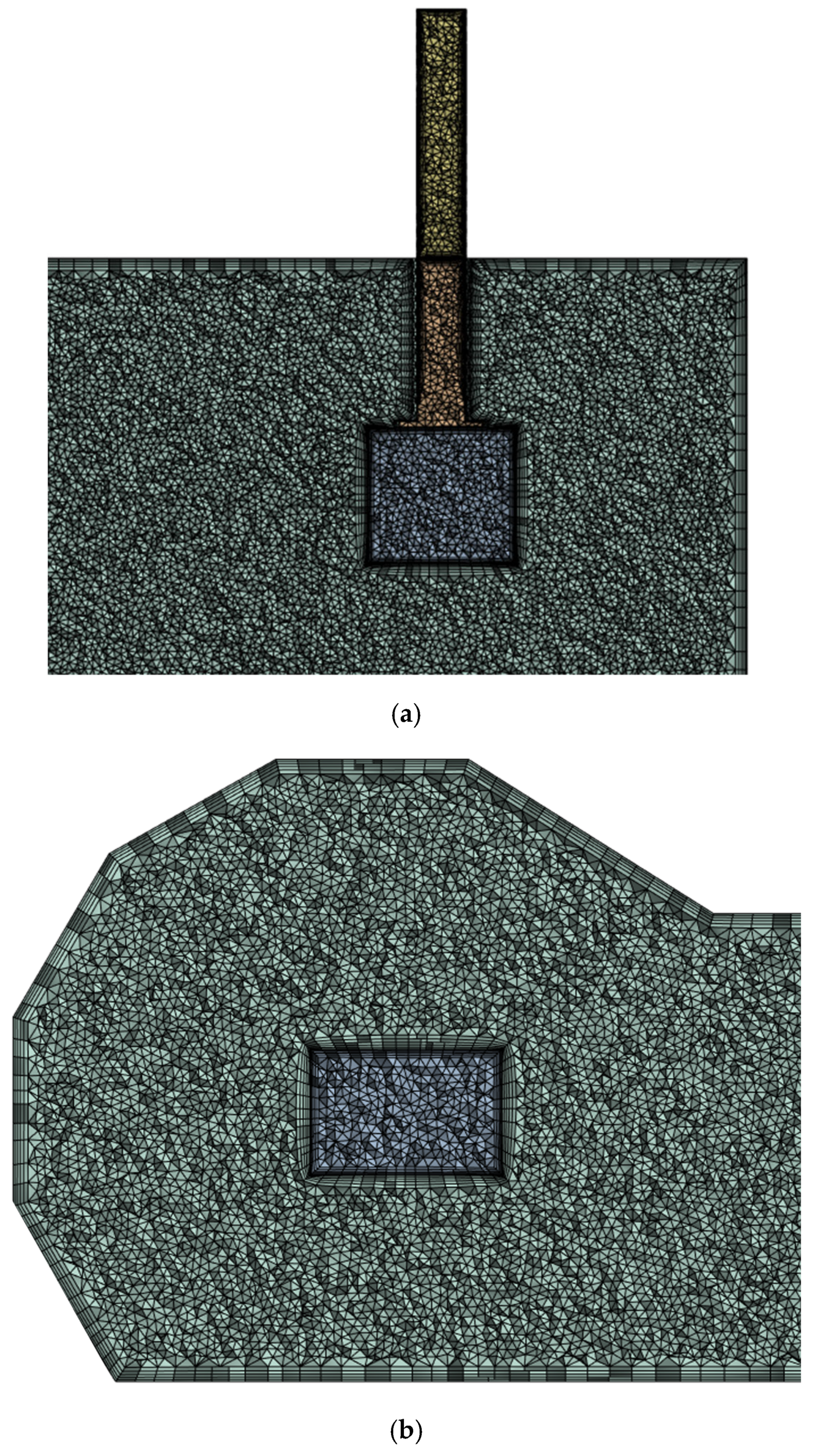
A mesh sensitivity analysis was performed to find a suitable computational mesh with a y+ value larger than 40 in order to ensure the wall function usage in CFX. For a simple transient case, the boundary conditions included a mass flow of 126 kg/s and a constant inlet temperature of 20 °C. The total time for the transient was 30 s. The time step used for the analysis was 0.5 s for the first 5 s and 5 s for the remaining time. The number of nodes, element quality, and Courant number for each mesh are summarized in Table 1. Based on the high minimum element quality and relatively low maximum Courant number, we concluded that the mesh used in Case 2 would provide a reasonable ratio between quality and computational effort. Therefore, this mesh was used for further calculations. It is important to note that the same y+ > 40 was used for all the cases shown in Table 1. The average y+ for the domain was 150. A graphical representation of mesh 2 in different parts of the model is shown in Figure 4.

Table 1.
Details of the mesh sensitivity analysis.
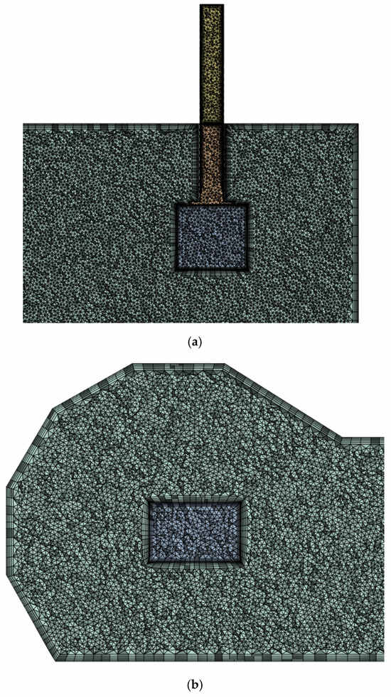
Figure 4.
Two different exemplary views of mesh 2 are shown. (a) shows a side cut of the mesh around the core, while (b) shows a top cut of the mesh around the core.
5.2. Boundary Conditions
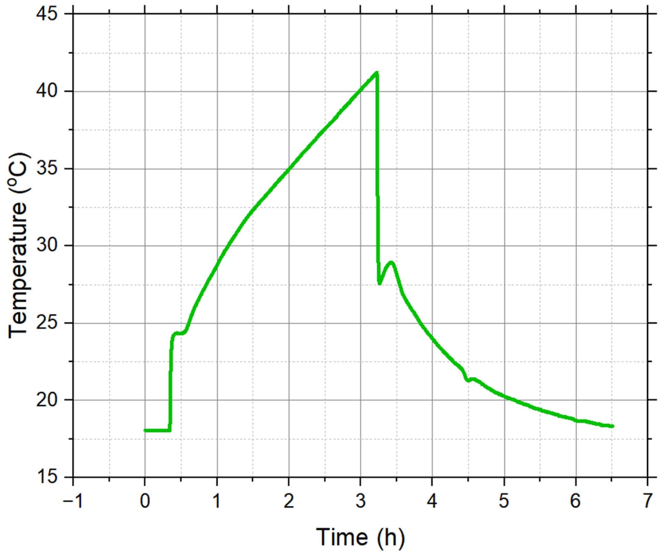
As already mentioned, the coolant inlet is located in pool 1 and the outlet in pool 2, just below the reactor core (see Figure 1). The mass flow of water used at the pool inlet is 126 kg/s, which was experimentally measured during the experiment, while the outlet pressure is set to 1.8 bar, a value that originates from MNR internal reports [7]. For the pool temperature transient simulation, the experimentally measured time-dependent temperature profile at the outlet of the heat exchanger was used as a boundary condition at the inlet. The profile used is shown in Figure 5.

Figure 5.
Time-dependent temperature profile extracted at the outlet of the heat exchanger. This profile is used as a boundary condition for the pool inlet temperature calculations.
Furthermore, an adiabatic free-slip wall boundary condition was used at the top surface of the pool, and an adiabatic no-slip wall boundary condition was used on the walls that would be in contact with the concrete housing. All walls were assumed to be hydraulically smooth, as wall roughness was assumed to play a negligible role in these simulations. No power is deposited in the core in this model, since the heat that the core deposits into the pool is already taken into account by the experimentally measured inlet temperature profile (shown in Figure 5). The IAPWS steam tables were used for the water properties [15].
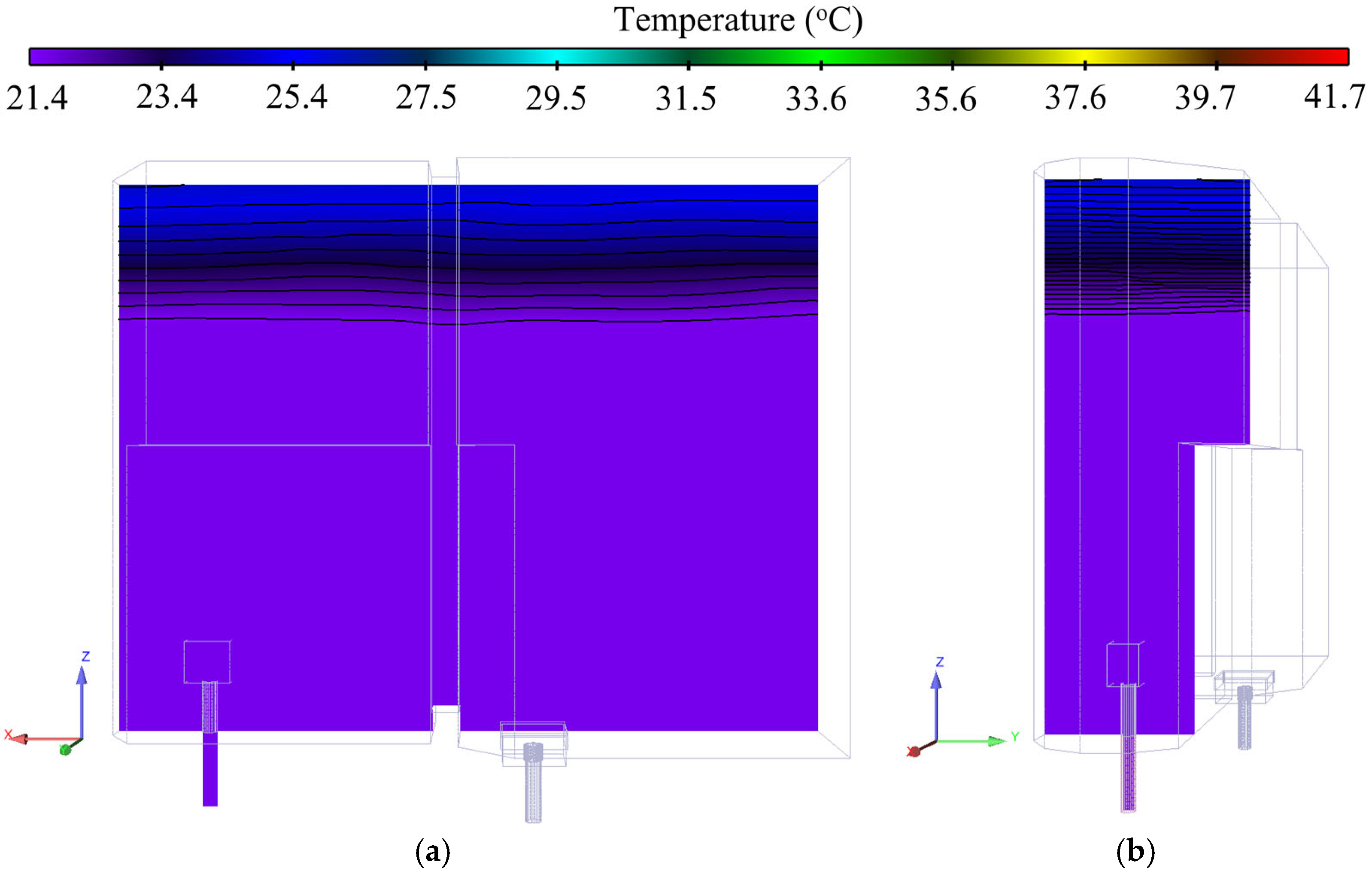
Prior to the pool mixing experiment at the MNR, the pool inlet temperature was gradually decreased over the course of 4 h from 28 °C to the lowest possible temperature, which corresponds to roughly 18 °C. Therefore, to simulate the experiment as accurately as possible, a preliminary calculation was performed, which will be described in very little detail here, as it is the focus of an ongoing publication [14]. This calculation was initialized with a homogeneous pool temperature of 28 °C, while the experimentally measured decrease in the inlet temperature was set as a boundary condition. This simulation led, on average, to a lower temperature as well as to the already mentioned stratification. A contour plot of the results yielded by the preliminary calculation is shown in Figure 6, where the flow stratification can be seen. The pool mixing transient, which is the focus of this paper, was initialized with the results of this previous cooling-down phase, as shown in Figure 6.

Figure 6.
Contour plot of the temperature profile used as the initial condition for the pool mixing transient shown at a front view (a) and side view (b).
The transient was run for 23,400 s (6.5 h), with a time step of 0.2 s for the first 20 s of the transient and 2 s for the remaining transient time. The results file, consisting of chosen variables, such as velocity, density, temperature, etc., was saved every 30 s. The total run time for this transient was 15,775 CPU hours. The residuals converged to smaller than 1 × 10⁻⁵.
6. Results and Discussion
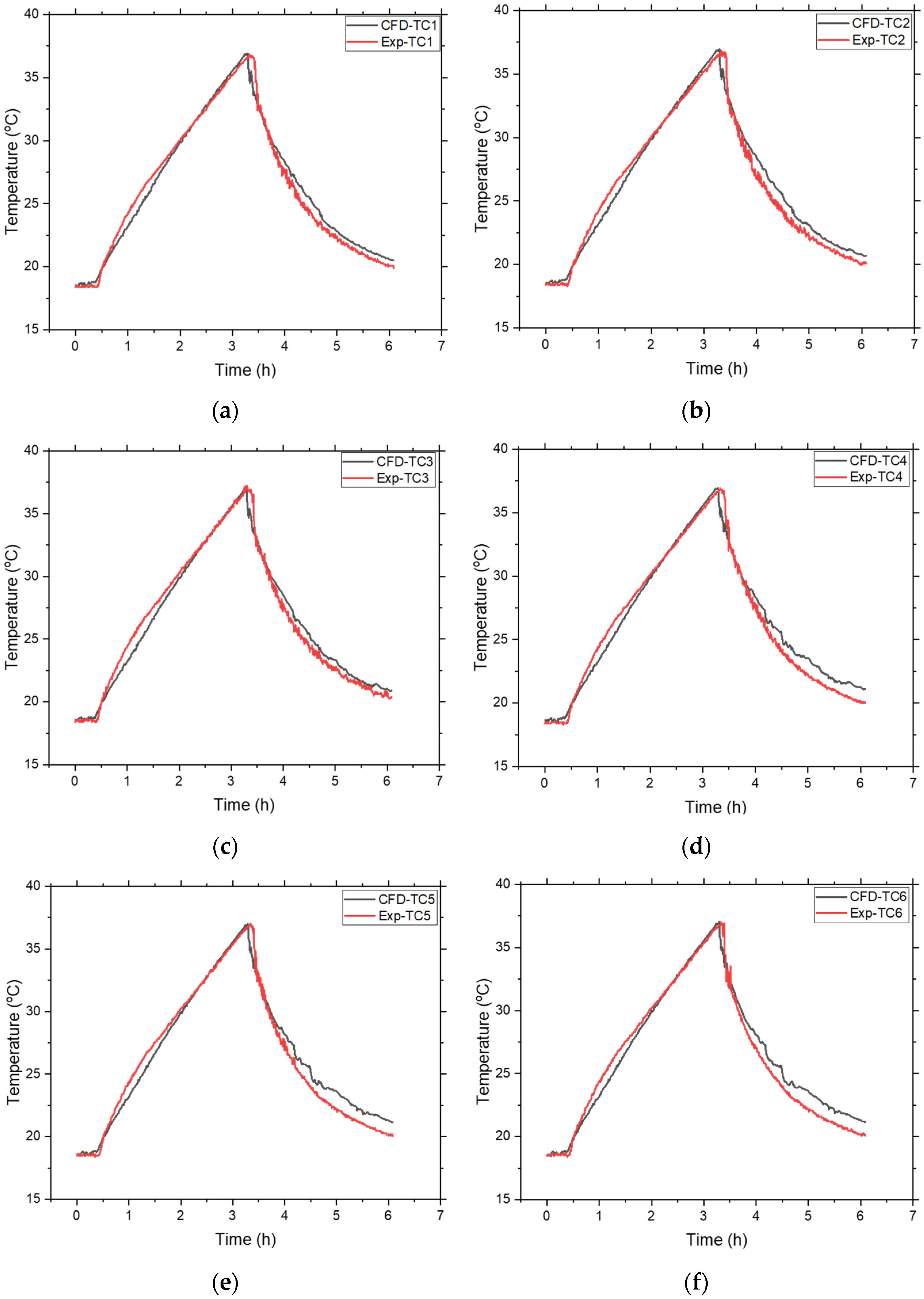
The temperature data measured by the installed thermocouples were compared to the data calculated by CFD for each thermocouple. The results are shown in Figure 7a–f. The maximum temperature calculated by CFD for each thermocouple matched very well with the measured values. The temperature calculated by CFD in the first 0.5 h of the transient was rather constant at 18.6 °C, with only small fluctuations in all thermocouple positions compared to the experimental values. The slope of the heating and cooling curves measured in the experiment was slightly nonlinear. However, this nonlinearity could not be reproduced by CFD. All the temperatures calculated in the thermocouple positions by CFD showed a slower increase during heating and cooling. This could be attributed to the fact that the various pool installations are not modeled in CFD. This means that the flow path calculated by CFD is shorter than in reality. Therefore, the water exits the computational domain faster than it would have done in the experiment. An additional reason could be that the reactor core and fuel elements were not explicitly modeled in CFD.
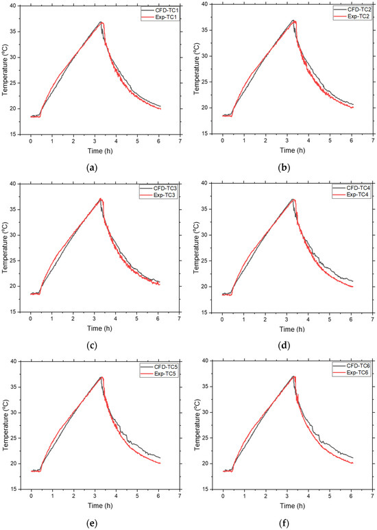
Figure 7.
Comparison of the data measured with the six thermocouples (also referred to as TC in the plots) in the experiments with the respective calculated temperatures in CFD. (a) Thermocouple TC1; (b) Thermocouple TC2; (c) Thermocouple TC3; (d) Thermocouple TC4; (e) Thermocouple TC5; (f) Thermocouple TC6.
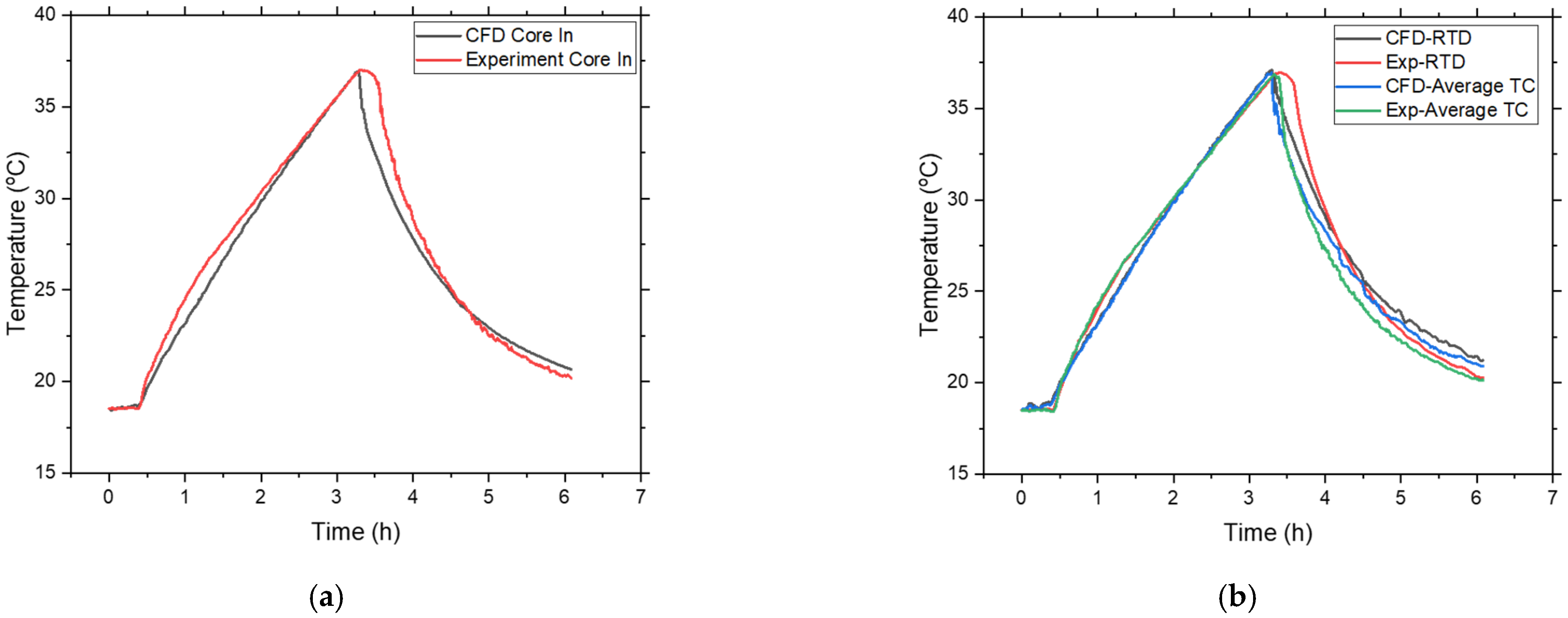
Figure 8a shows the time evolution of the water temperature at the core inlet for both the experiment and CFD. In addition to the difference in slope between the experiment and CFD during the heating and cooling observed for the thermocouples (see Figure 7), the broader peak measured in the experiment could not be reproduced in CFD. In reality, the core does not react immediately to the pool inlet temperature drop due to the thermal inertia of the pool installations. Also, the feedback from the neutronics due to the cooler coolant and the subsequent control adjustments are not modeled here, since the core is not modeled in CFD. Therefore, a sort of delay cooling can be observed in the experiment once the secondary pumps are turned back on.
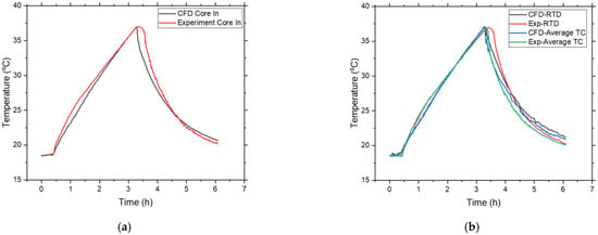
Figure 8.
(a) Temperature development over time at the core inlet measured in the experiment and calculated by CFD. (b) Comparison of the temperature at the RTD position and thermocouples measured in the experiment and calculated by CFD.
Figure 8b shows the comparison between the experiment and CFD regarding the RTD position temperature, together with a comparison between the average temperature measured by the thermocouples in the experiment and the average calculated temperature in CFD. The RTD is located vertically farther away from the core, about 1.5 m (see Figure 3a,b). When the pool inlet temperature declines drastically, the warm water moves toward the pool surface due to density changes. Therefore, the RTD’s reaction to the cooling down is somewhat delayed. This can be seen in the experimental results. Even though there is a small broadening of the peak in the CFD results, the response of the RTD temperature to the cooling is faster than in the experiment.
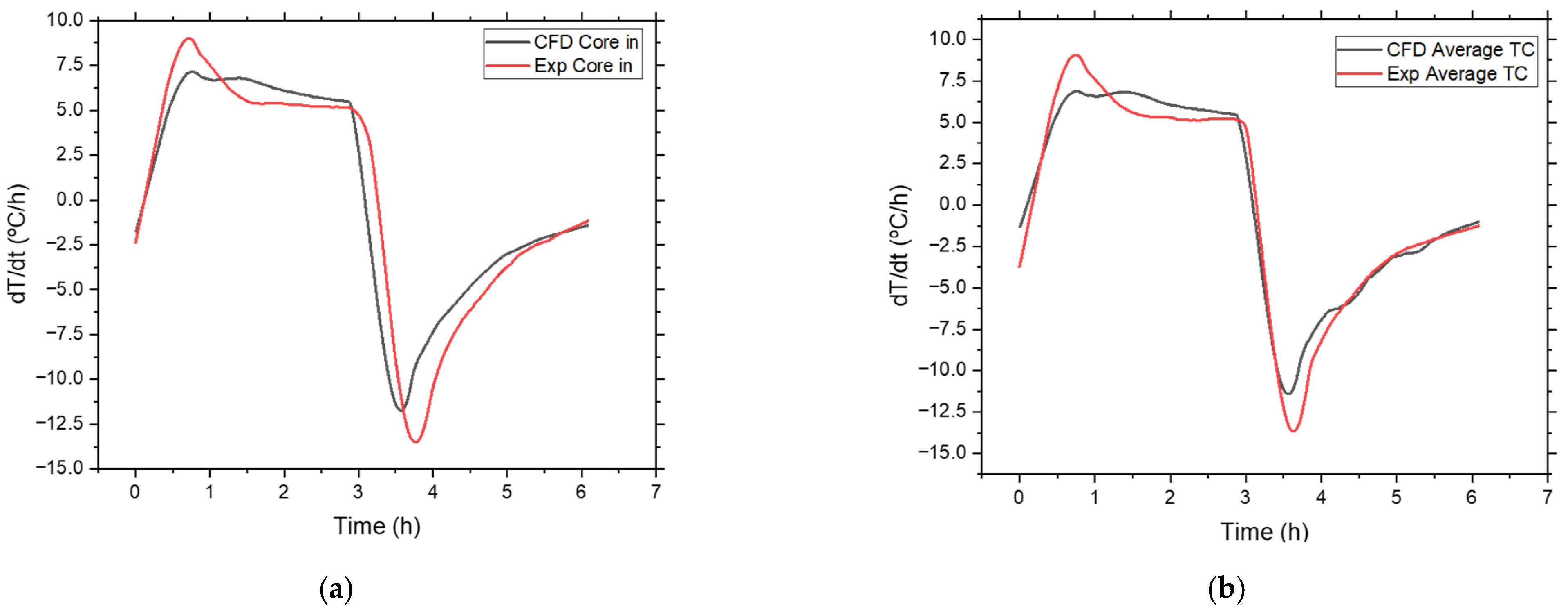
To better visualize the change in pool temperature, the derivatives of the core inlet temperature and the average thermocouple temperature are shown in Figure 9a,b, respectively. For the first 0.5 h, the temperature derivative at the core inlet is very similar between the CFD and the experiment. After 0.5 h, the core inlet temperature measured in the experiment increases faster than the one calculated by CFD. At about 2 h, the rate of temperature change in the experiment reaches a plateau at about 5.3 °C/h. In the CFD results, the heating rate slows down to around 5.5 °C/h.
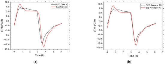
Figure 9.
(a) Comparison of the derivative of the core inlet temperature between the experiment and CFD. (b) Comparison of the derivative of the average thermocouple temperature between the experiment and CFD.
At t = 3 h, the secondary heat removal system restarts, and therefore, the pool inlet temperature decreases. This is reflected in Figure 9a by the steep decrease in the temperature derivative. Since the core is not modeled in CFD, the derivative of the core inlet temperature calculated by CFD (black curve) declines faster than that from the experiment. The derivative of the core inlet temperature from the experiment (red curve) is slower to react to the restart of the secondary heat removal system due to the thermal inertia of the core. At the end of the transient, the rate of cooling for both the experiment and CFD is the same. A similar situation is depicted in Figure 8b for the derivative of the thermocouples’ average temperature.
The experimental values of both the core inlet temperature and the average thermocouple temperature drop further down, which strengthens the point that the missing thermal inertia in the CFD simulations is responsible for most of the differences between the simulation and the experiment.
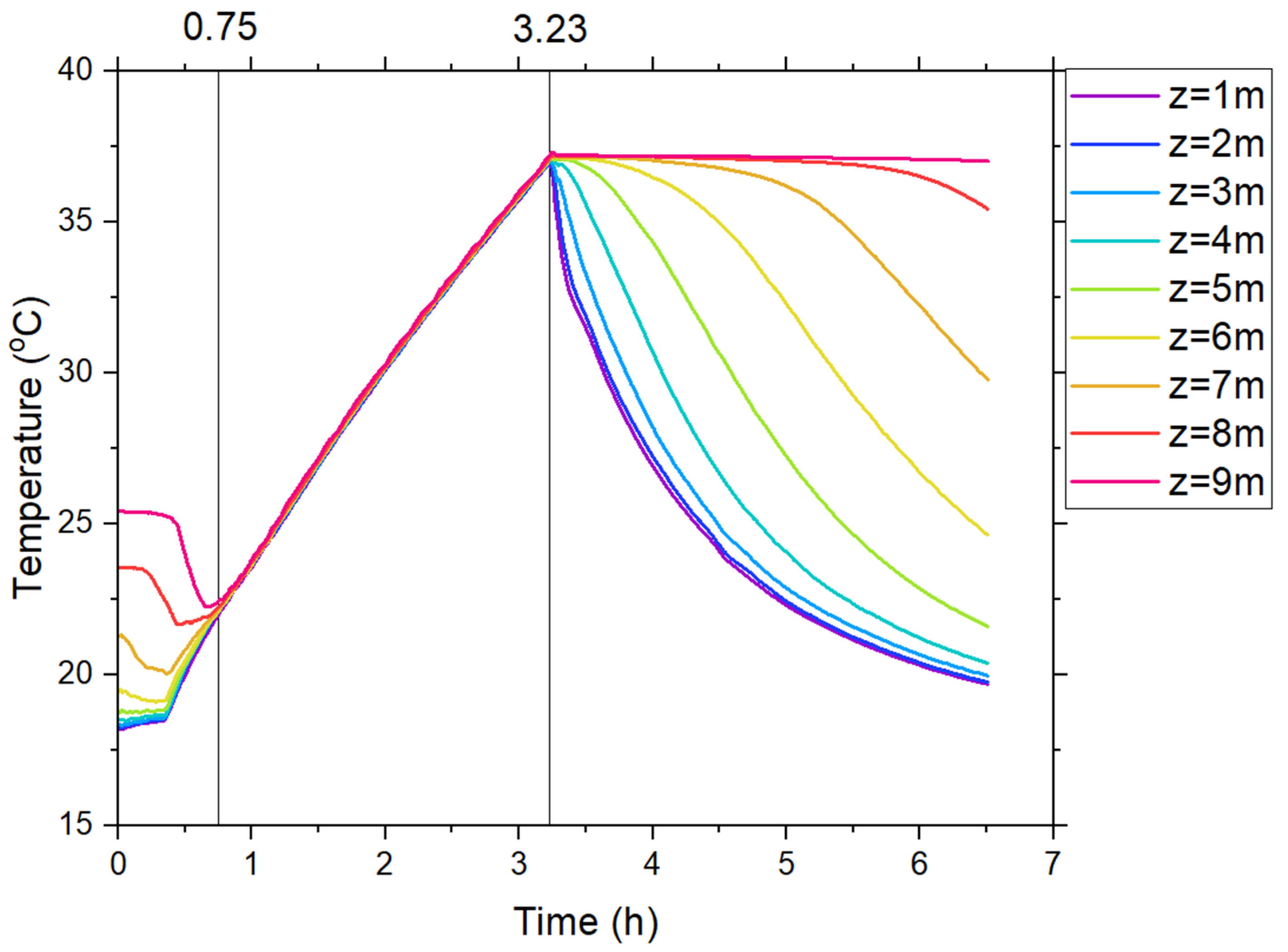
Figure 10 shows the area-averaged water temperature calculated at different heights from the bottom of the pool. From the beginning of the transient until t = 0.75 h, the averaged water temperature reflects the initial conditions of the pool stratification, with the temperature being higher at the top of the pool and lower at the bottom. During the heating cycle, the average water temperatures are consistent at all heights of the pool. Additionally, the time evolution of the average temperature is identical at all heights. When the secondary cooling restarts at t = 3.23 h, the warm water, once located at the bottom of the pool, moves to the top due to density changes, and colder water coming into the pool inlet occupies its place.
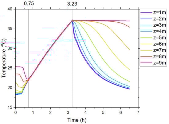
Figure 10.
Area-averaged water temperature at different heights from the bottom of the pool.
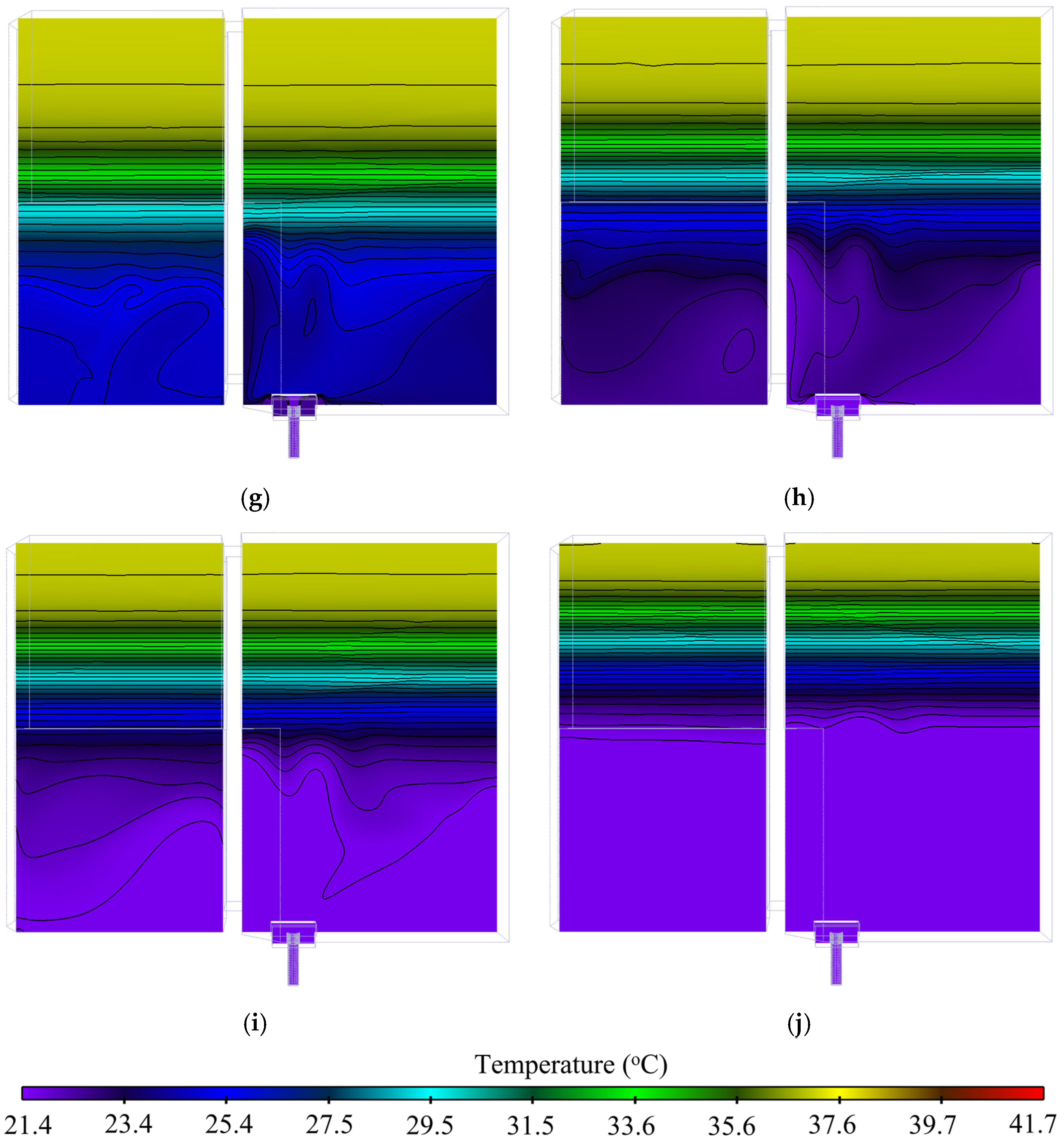
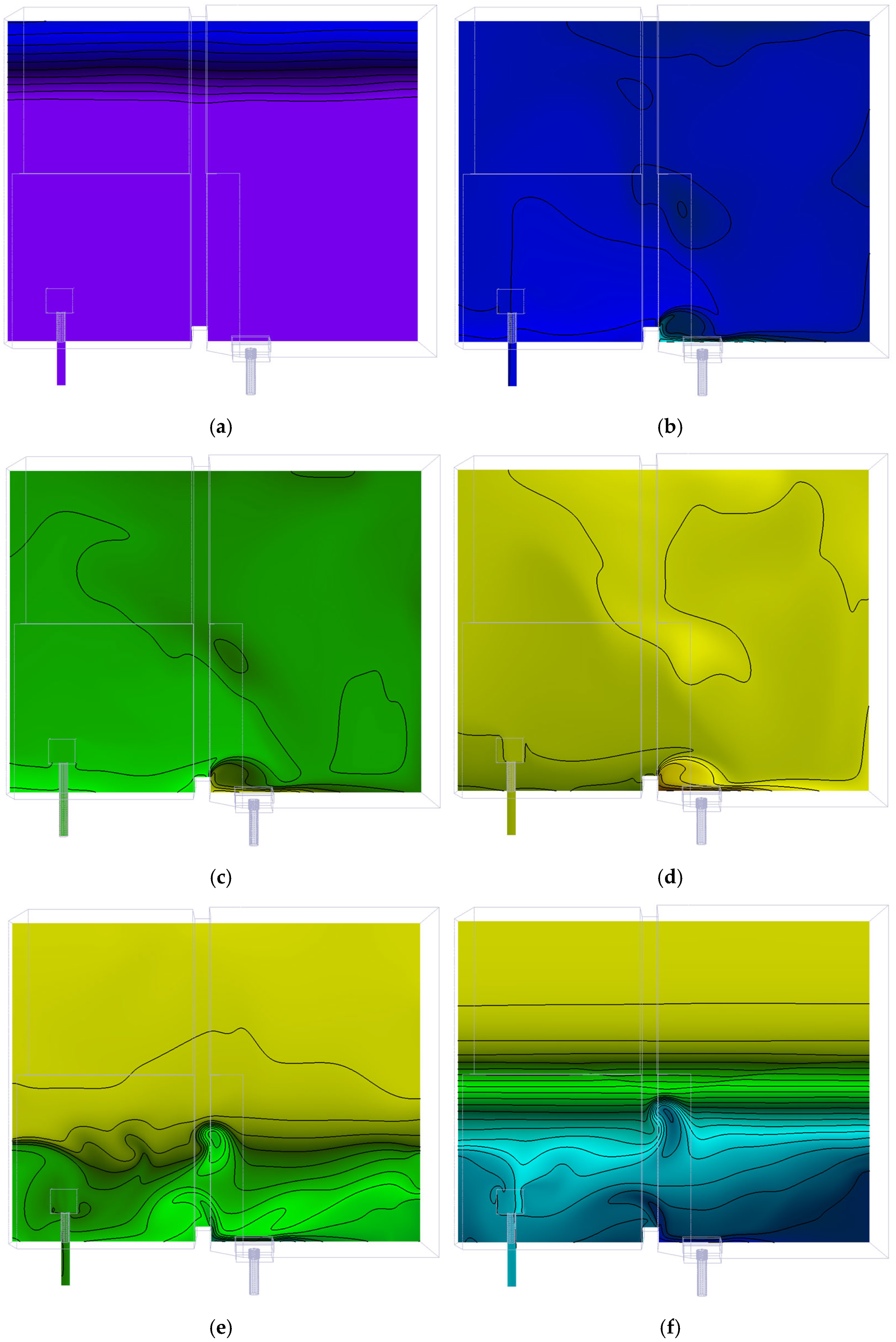
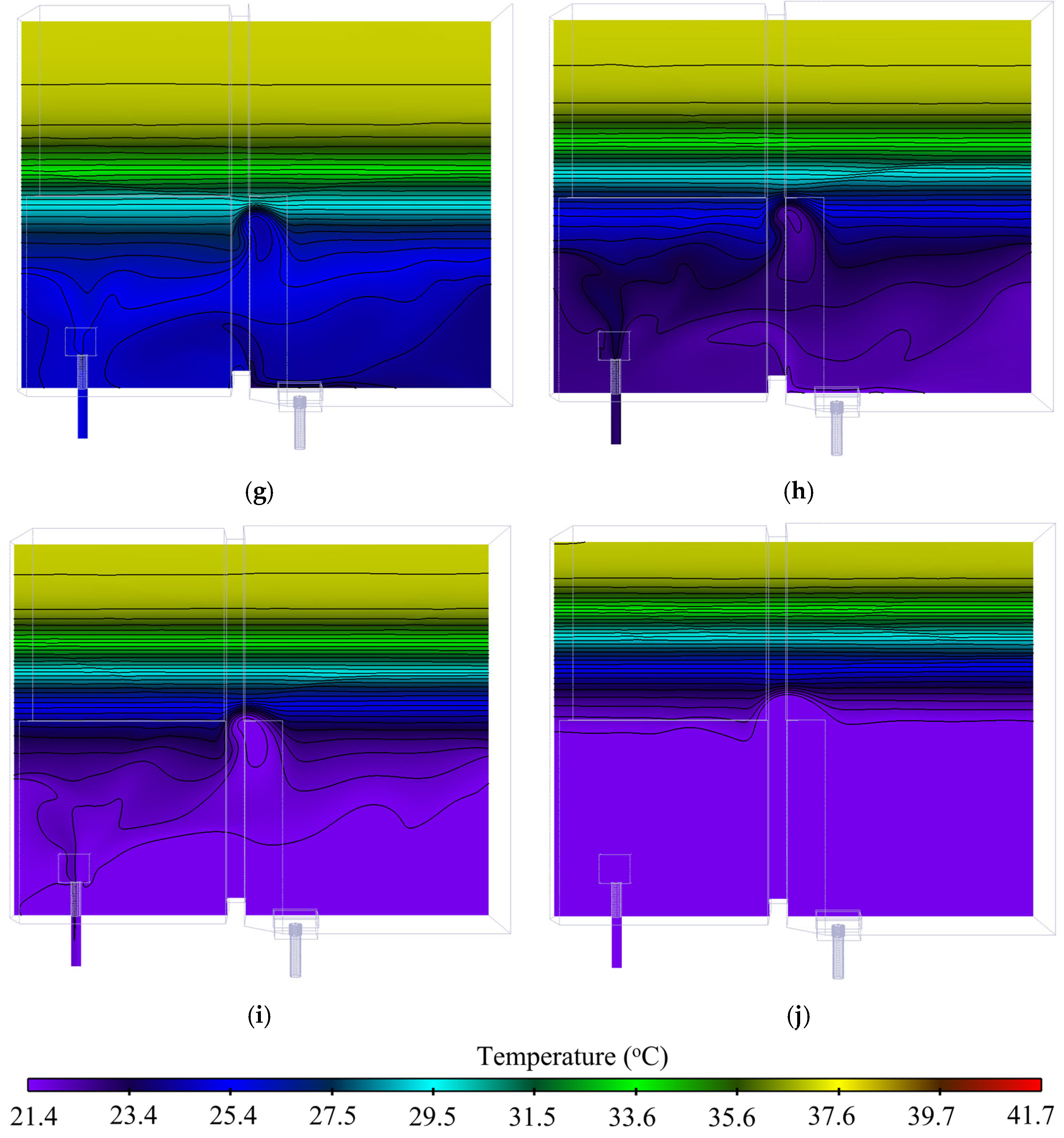
Figure 11a–j show the water temperature at an xy-plane cutting through the inlet at different time steps. The contours in Figure 11a–c show the pool temperature during the heating cycle. The temperature contours during the cooling down are shown in Figure 11d–j. During the heating cycle, the water mixing is very efficient and rather homogeneous (as also seen in Figure 6) since the heating occurs gradually. However, the cooling is rather abrupt, which leads to non-homogeneous water mixing, especially at t = 3.33 h and t = 3.88 h, also shown in Figure 11e,f. In the last 2 h of the transient, the temporal evolution of the inlet temperature is slower, which implies better mixing. At the end of the transient, more than half of the bottom part of the pool has a constant temperature of roughly 21 °C, as shown in Figure 11j.
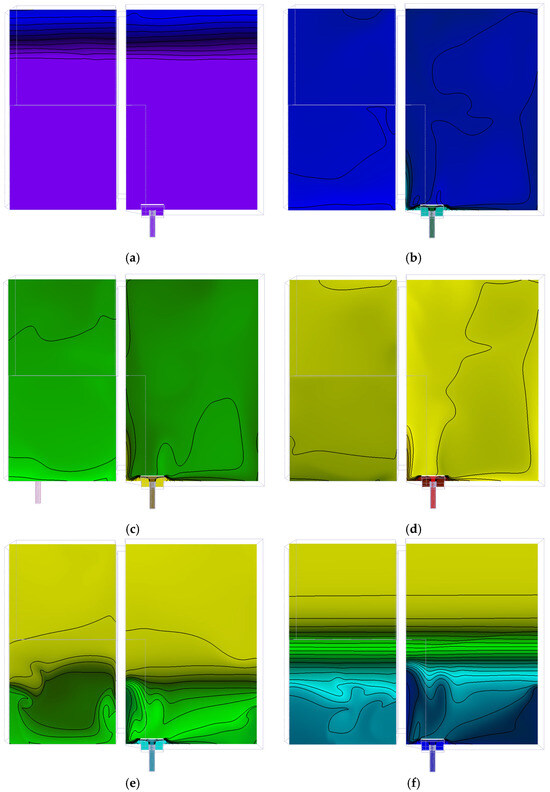
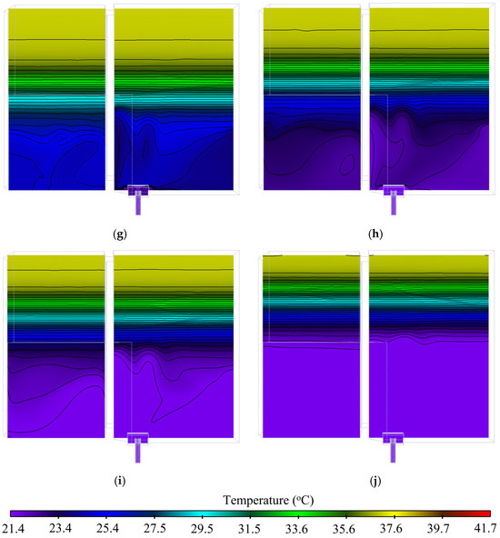
Figure 11.
Temperature contours of the plane located in the middle of the inlet at different times of the transient: (a) 0 h, (b) 1.388 h, (c) 2.77 h, (d) 3.22 h, (e) 3.33 h and (f) 3.88 h, (g) 4.44 h, (h) 5 h, (i) 5.55 h and (j) 6.76 h.
The temperature contours at a plane cutting through the core are shown in Figure 12a–j for the same time steps as in Figure 11. It can be concluded that the temperature contours at a plane cutting through the core, as shown in Figure 12a–j for different time steps, yield the same results. The wave-like pattern observed in the middle of the pool during the cooling down phase is due to the pool inlet’s structure and location. The cold water entering the pool is distributed around the diffusor, which is located near the pool walls on one side. As a result, the cold water collides with the concrete walls, causing a wave-like structure. This “wave” is almost nonexistent at the end of the transient, as shown in Figure 12j. A more detailed view of this wave is shown with contours in Figure 13a during the heating and Figure 13b during the cooling.
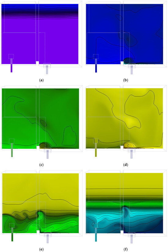
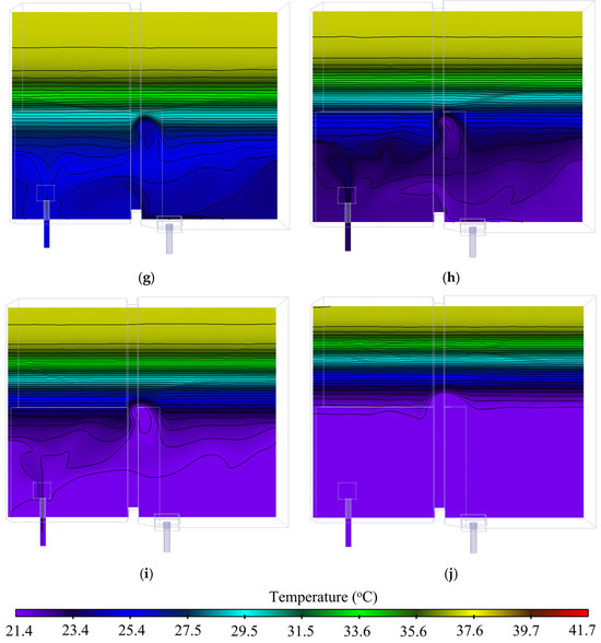
Figure 12.
Temperature contours of the plane located in the middle of the core at different times of the transient: (a) 0 h, (b) 1.388 h, (c) 2.77 h, (d) 3.22 h, (e) 3.33 h and (f) 3.88 h, (g) 4.44 h, (h) 5 h, (i) 5.55 h and (j) 6.76 h.

Figure 13.
Contour plots depicting the thermal “wave” in different yz planes of the pool at (a) t = 2.77 h and (b) t = 3.88 h.
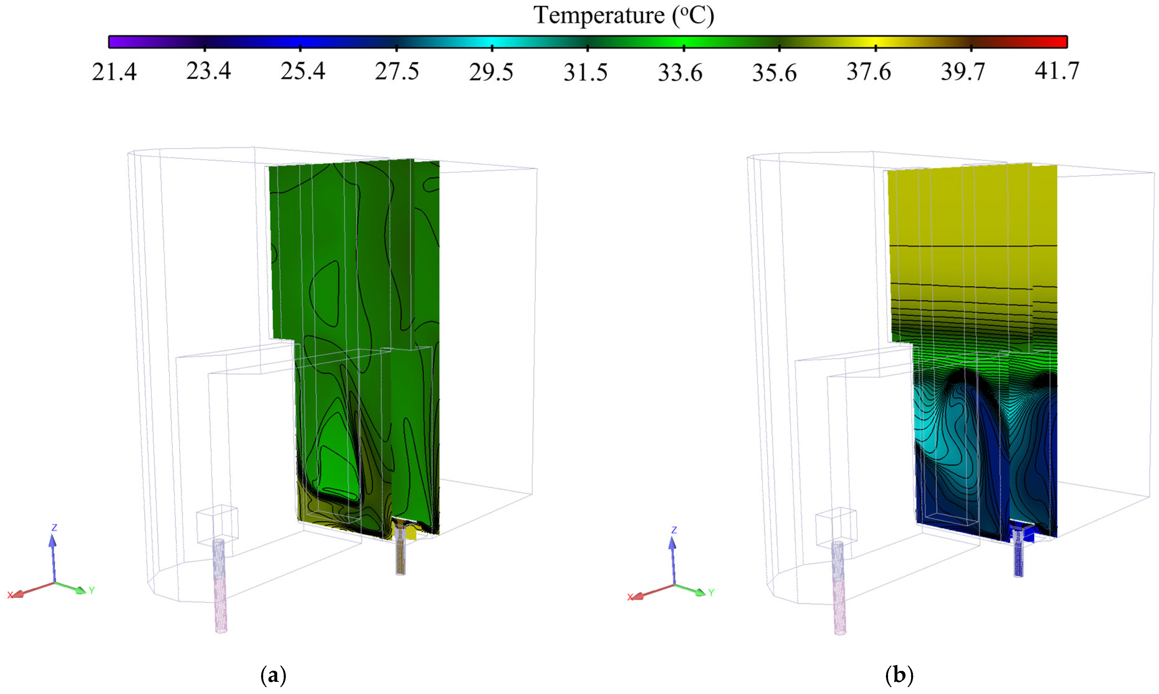
The 3D flow pattern is shown in Figure 14 for t = 1.388 h and t = 3.88 h at a plane cutting through the core. As seen in Figure 14, severe mixing occurs at all heights of the pool at t = 1.388 h, while at t = 3.88 h the warmer water has moved to the upper part of the pool and the mixing occurs at the pool bottom.
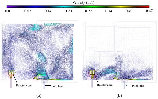
Figure 14.
3D flow pattern for (a) t = 1.388 h and (b) t = 3.88 h.
Taking into account all the results shown in the previous figures, it can be stated that CFD manages to capture well the events of the pool mixing experiment at the MNR. This conclusion is drawn after taking into account the simplifications made to the model geometry, such as not modeling the core explicitly and not including the concrete containment and other thermal inertia. An additional point to be made is the fact that in the present work, no uncertainties are calculated nor stated regarding the experimental results. However, due to the equipment used, the experimental uncertainties are expected to be in the range of 3–5%, but data processing is still ongoing. For a more detailed representation of the pool experiment with CFD, the model would have to take into account the core and the concrete housing of the pool. However, such a task is cumbersome and impractical for a 7 h transient with a multimillion-node mesh. Therefore, the CFD modeling can be focused on a fraction of the pool experiment in the future.
7. Conclusions and Outlook
The loss of heat sink scenario for the MNR was analyzed through CFD simulation and compared with experimental data for validation purposes. The results indicate that despite the simplifications assumed during the analysis, the CFD model manages to capture the thermal mixing in the MNR pool well. Additionally, the temperatures of the coolant measured by the thermocouples can be accurately reproduced by CFD. The outcome provided by the CFD modeling contributes to the improvement of system code modeling for the safety analysis of the MNR as well as to inform the measurements of spatial gradients, in particular near the time when cooling is initiated. In the near future, the explicit modeling of the MNR’s fuel assemblies will be useful for validating the conjugate heat transfer aspect of CFD and for assessing the safety of the MNR core. Additionally, the repetition of the loss of heat sink experiment in the MNR with multiple thermocouple rakes in different positions and heights of the pool is part of the near-future goals. A detailed neutronic assessment of the core behavior during the transient should be performed, especially to quantify the temperature feedback coefficient of the reactor.
Author Contributions
Conceptualization, K.S. and C.R.; software validation: K.S.; formal analysis: K.S. and K.R., investigation: K.S. and K.R.; data resources: K.R., T.S., S.D., R.P. and C.R.; data curation: K.S., K.R., R.P. and T.S.; writing-original draft preparation: K.S.; writing-review and editing: K.R., K.S., C.R., D.N. and T.S.; visualization: K.S. and C.R.; supervision: C.R. and D.N.; project administration: C.R. and D.N.; funding acquisition: C.R. and D.N. All authors have read and agreed to the published version of the manuscript.
Funding
Technische Universität München work was supported through a combined grant (FRM2023) from the Bundesministerium für Bildung und Forschung (BMBF) and the Bayerisches Staatsministerium für Wissenschaft und Kunst (StMWK). McMaster University houses a robust suite of nuclear infrastructure, including a 5 MW research reactor, 16.5 MeV cyclotron, post-irradiation facilities, and nuclear research laboratories, driving discoveries in nuclear energy, materials research, and medical isotopes.
Data Availability Statement
The experimental data used for validation will be published as part of an IAEA Control Research project titled “Development of Coupled Neutronic and Thermal-Hydraulic Calculational Methodologies for Research Reactors including Analysis and Treatment of Uncertainties”.
Acknowledgments
The authors would like to express their gratitude to Andreas Kloh for generating the CAD model, as well as to Dave Tucker, Derek Cappon, and all the people who supported this experiment. The authors thank McMaster University’s Nuclear Operations and Facilities for their support in conducting the necessary experiments for this paper.
Conflicts of Interest
The authors declare no conflicts of interest.
References
- Zhang, H.; Andrs, D.; Hansel, J.; Zou, L.; Berry, R.; Martineau, R. RELAP-7 User’s Guide; INL/EXT-14-33977-Rev001; Idaho National Lab. (INL): Idaho Falls, ID, USA, 2018. Available online: https://www.osti.gov/servlets/purl/1466669 (accessed on 1 April 2024).
- Préa, R.; Fillion, P.; Matteo, L.; Mauger, G.; Mekkas, A. (Eds.) CATHARE-3 V2.1: The New Industrial Version of the CATHARE Code. In Proceedings of the ATH’2020-Advances in Thermal Hydraulics Conference, Palaiseau, France, 20–23 October 2020; American Nuclear Society (ANS): Westmont, IL, USA, 2020. [Google Scholar]
- Lizzoli, M.; Borreani, W.; Devia, F.; Lomonaco, G.; Tarantino, M. Preliminary CFD Assessment of an Experimental Test Facility Operating with Heavy Liquid Metals. Sci. Technol. Nucl. Install. 2017, 2017, 1949673. [Google Scholar] [CrossRef]
- Gao, X.; Carasik, L.B.; Coble, J.B.; Hines, J.W. A New Development of Cross-Correlation-Based Flow Estimation Validated and Optimized by CFD Simulation. Appl. Sci. 2024, 14, 6687. [Google Scholar] [CrossRef]
- International Atomic Energy Agency. Safety Assessment for Research Reactors and Preparation of the Safety Analysis Report. 978-92-0-141521-9. Available online: https://www-pub.iaea.org/MTCD/Publications/PDF/PUB1981_web.pdf (accessed on 1 April 2024).
- International Atomic Energy Agency (IAEA). Development of Neutronic and Thermal-Hydraulic Coupled Calculational Methodologies for Research Reactors Including Treatment of Uncertainties; IAEA: Vienna, Austria, 2022. [Google Scholar]
- Blahnik, C.; Blahnik. Safe Operating Envelope of McMaster Nuclear Reactor; McMaster Nuclear Reactor: Hamilton, ON, Canada, 2020. [Google Scholar]
- Ansys. Ansys CFX Solver Theory Guide. Release 2024.R1. In Ansys User Guide; ANSYS, Inc.: Canonsburg, PA, USA, 2024; p. 1. [Google Scholar]
- McMaster University. McMaster Nuclear Reactor Safety Report; McMaster University: Hamilton, ON, Canada, 2002. [Google Scholar]
- Reynolds, O., IV. On the dynamical theory of incompressible viscous fluids and the determination of the criterion. Philos. Trans. R. Soc. A 1895, 186, 123–164. [Google Scholar] [CrossRef]
- Menter, F.R. Two-equation eddy-viscosity turbulence models for engineering applications. AIAA J. 1994, 32, 1598–1605. [Google Scholar] [CrossRef]
- Menter, F.R.; Kuntz, M.; Langtry, R. Ten years of industrial experience with the SST turbulence model. Heat Mass Transf. 2003, 4, 625–632. [Google Scholar]
- Shehu, K.; Bojanowski, C.; Bergeron, A.; Petry, W.; Reiter, C. First Steps to Coupled Hydraulic and Mechanical Calculations within a Parameter Study to Define Possible Core Designs for the Conversion of FRM II. EPJ Web Conf. 2021, 247, 8011. [Google Scholar] [CrossRef]
- Ruiz, K.; Shehu, K.; Novog, D.; Reiter, C.; Day, S.; Schlitt, T.; Pasuta, R. Pool Temperature Experiment: Validating the RELAP5 code for the initial stages of a Loss of Heat Sink Accident in the McMaster Nuclear Reactor. Nucl. Eng. Des. 2024. in review process. [Google Scholar]
- Wagner, W.; Kruse, A. The Industrial Standard IAPWS-IF97 for the Thermodynamic Properties and Supplementary Equations for Other Properties; Springer: Berlin/Heidelberg, Germany, 1998. [Google Scholar]


Disclaimer/Publisher’s Note: The statements, opinions and data contained in all publications are solely those of the individual author(s) and contributor(s) and not of MDPI and/or the editor(s). MDPI and/or the editor(s) disclaim responsibility for any injury to people or property resulting from any ideas, methods, instructions or products referred to in the content. |
© 2024 by the authors. Licensee MDPI, Basel, Switzerland. This article is an open access article distributed under the terms and conditions of the Creative Commons Attribution (CC BY) license (https://creativecommons.org/licenses/by/4.0/).