Fault-Line Selection Method in Active Distribution Networks Based on Improved Multivariate Variational Mode Decomposition and Lightweight YOLOv10 Network

Abstract

In active distribution networks (ADNs), the extensive deployment of distributed generations (DGs) heightens system nonlinearity and non-stationarity, which can weaken fault characteristics and reduce fault detection accuracy. To improve fault detection accuracy in distribution networks, a method combining improved multivariate variational mode decomposition (IMVMD) and YOLOv10 network for active distribution network fault detection is proposed. Firstly, an MVMD method optimized by the northern goshawk optimization (NGO) algorithm named IMVMD is introduced to adaptively decompose zero-sequence currents at both ends of line sources and loads into intrinsic mode functions (IMFs). Secondly, considering the spatio-temporal correlation between line sources and loads, a dynamic time warping (DTW) algorithm is utilized to determine the optimal alignment path time series for corresponding IMFs at both ends. Then, the Markov transition field (MTF) transforms the 1D time series into 2D spatio-temporal images, and the MTF images of all lines are concatenated to obtain a comprehensive spatio-temporal feature map of the distribution network. Finally, using the spatio-temporal feature map as input, the lightweight YOLOv10 network autonomously extracts fault features to achieve precise fault-line selection. Experimental results demonstrate the robustness of the proposed method, achieving a fault detection accuracy of 99.88%, which can ensure accurate fault-line selection under complex scenarios involving simultaneous phase-to-ground faults at two points.

1. Introduction

The most common fault in the power system is a single-phase grounding fault. The distribution network is an important part of the power system, and its safe and stable operation is closely related to people’s lives [1]. China’s low and medium voltage distribution network is widely used in small current grounding; however, the incidence of single-phase grounding faults in small current grounding systems is as high as more than 80%. If the fault is not cleared in a timely manner, it may result in insulation breakdown, triggering multiphase and multipoint faults [2]. With the advancement and development of the new type of ADNs, a multitude of DGs are integrated into the distribution network, which makes the structure of the distribution network complicated. And the characteristics and distribution of the zero-sequence currents during faults have changed significantly [3], so the traditional fault-line model of the distribution network is no longer applicable. Therefore, it is urgently needed to analyze fault characteristics of new distribution networks and study the effective methods for fault lines in ADNs.

In recent years, extensive research has been performed on fault-line selection in distribution networks with ineffective neutral grounding. Various methods have been proposed, categorized into passive, active, and integrated methods based on whether fault characteristic information originates from the fault itself. Passive methods include steady-state information-based methods [4] and transient information-based methods, etc. [5]. Active methods utilize externally injected signals to identify faults [6], such as signal injection, small disturbance, residual flow increment methods, etc. [7]. Integrated methods combine different approaches of modern information processing technologies for fault-line selection. References [8,9] decompose the fault current by wavelet transform and extract the eigenvalues of fault information for fault-line selection, but the wavelet transform requires fine parameter adjustments, as the selection of the wavelet basis function, the selection of the scale parameter has a large impact on the fault-line selection results, and the methods requires a large amount of computational resources and time, especially in the real-time system, which may not be able to satisfy the demand for immediate processing. Reference [10] proposed a protection strategy using an extended Kalman filter to detect various types of DC faults using only the current signals in the medium voltage DC distribution network to achieve fault-line selection. However, this method requires low-frequency wireless communication capability for smart grids, and the sensitivity to ambient noise and uncertainty remains to be thoroughly investigated. Reference [11] proposes the use of transient negative sequence currents for fault-line selection, which is not affected by capacitive unbalance and transition resistance, and also solves the defects of zero-sequence currents in the presence of underground cables. However, the negative sequence currents are affected by load imbalance and are not applicable to distribution networks containing DGs. Reference [12] introduced a method of selecting the line of faults by modifying the complete ensemble empirical mode decomposition (MCEEMD) and the duffing system, which is less affected by fault types and transient resistances. Yet, noise signals can lead to classification errors, affecting the system’s robustness. In [13], the authors combined injection methods with variational mode decomposition (VMD) to use relative entropy of energy as a criterion for fault-line selection. However, VMD requires pre-setting the number of decomposition layers, potentially influencing fault-line selection outcomes if improperly chosen. The authors of [14] utilized different detection methods to extract multiple features and integrated them using fuzzy theory for fault-line selection. This approach demonstrates strong generalization capabilities for identifying various fault types but increases computational complexity and time costs, rendering it less efficient in practical applications.

In recent years, the rapid development of artificial intelligence has led to widespread applications of machine learning in fault identification within distribution networks, such as k-means clustering algorithm [15], support vector machines (SVMs) [16], and extreme learning machines (ELMs) [17]. However, these methods have a certain degree of subjectivity in extracting fault feature vectors and rely on research experience in related fields. Improper extraction of feature vectors will seriously affect the validity of the diagnosis. Deep learning has seen outstanding achievements in areas such as image identification due to its capability to extract deep features autonomously from raw data. Reference [18] extracts the energy value characteristics of current signals and uses long short-term memory (LSTM) neural networks to classify and identify fault lines, which has a good effect on detecting high-impedance faults, but LSTM has certain limitations on the length of the input sequence, and when the sequence length is long, the LSTM may have the problem of gradient disappearance or gradient explosion, which makes it difficult to effectively capture the dependence of long distances. In [19], the first half wave of zero-sequence current is fused into waveforms, and a one-dimensional convolutional neural network (CNN) is utilized to extract the significant fault features of the fused waveforms, thus realizing fault-line selection. However, the direct use of one-dimensional fault feature signals ignores the spatial and temporal correlation of the original signals and fails to give full play to the advantages of deep learning in the field of image recognition. Reference [20] uses existing signal processing techniques to transform 1D signals into 2D feature images and inputs them into CNN for feature extraction to complete the fault-line selection. But this method overlooks the global features of the original signal, incurs high time and computational costs, and is not applicable to the scenarios of resource constraints and real-time detection.

Table 1. Comparison and summary of different line selection methods.

Category	Methods	References	Schemes of Fault-Line Selection	Advantage	Limitations
Classified by fault characteristics	Zero-sequence current method	Refs. [8,9]	Wavelet transform	Suitable for many types of faults, high accuracy for high-resistance grounding	Selection of wavelet basis functions is empirically dependent and computationally and time-costly
		Ref. [10]	Extended Kalman filters	Suitable for multiple topologies and different types of faults with short operating times	Weak anti-interference capability
		Ref. [12]	MCEEMD and Duffing system	Independent of fault type, transition resistance	Susceptible to noise interference
	Negative sequence current method	Ref. [11]	Moving average method	Unaffected by capacitor imbalance and transition resistance	Vulnerable to load imbalance and not applicable to distribution networks containing DGs
	Injection method	Ref. [13]	VMD and energy relative entropy	Unaffected by transition resistance, strong anti-interference ability	The selection of the number of decomposition layers of the VMD preset affects the line selection results
	Integrated methods	Ref. [14]	Multi-feature fusion based on fuzzy theory	Strong generalization capabilities	High computational complexity and time cost
Classified by fault feature extraction methods	LSTM	Ref. [18]	LSTM mines the energy value characteristics of the current signal	High accuracy for high-resistance faults	Difficulty in effectively capturing long-distance dependencies
	1D-CNN	Ref. [19]	1D-CNN extracts the significant fault features of the fused	Strong anti-interference ability	Neglecting the spatio-temporal correlation of the original signal
	2D-CNN	Ref. [20]	The 1D signal is converted into a 2D image, and the fault features are extracted by 2D-CNN	Give full play to the advantages of deep learning in the field of image recognition	Lack of global characterization and high computational cost

shows the comparison and summary of different line selection methods in the above references.

This paper proposes a method for fault-line selection in distribution networks with DGs based on IMVMD and a lightweight YOLOv10 network. Initially, IMVMD decomposition is applied to zero-sequence currents at the source and load ends to extract a series of IMFs. These IMFs from the source and load ends are aligned, using DTW to establish optimal alignment paths of 1D time series. The MTF transformation is then employed to convert the 1D sequences into 2D images, enriching fault feature information and enabling visualization. To fully consider spatio-temporal correlations, all MTF images are concatenated to construct a spatio-temporal feature map of the distribution network. Finally, the fault lines on the spatio-temporal feature map are annotated and input into the lightweight YOLOv10 network for autonomous fault feature exploration to complete the fault-line selection process. This method effectively enhances the accuracy and robustness of fault-line selection in ADNs.

This paper focuses on fault feature signal processing and fault feature autonomous mining when a single-phase ground fault occurs in ADNs, and the main research work is summarized as follows:

(1)

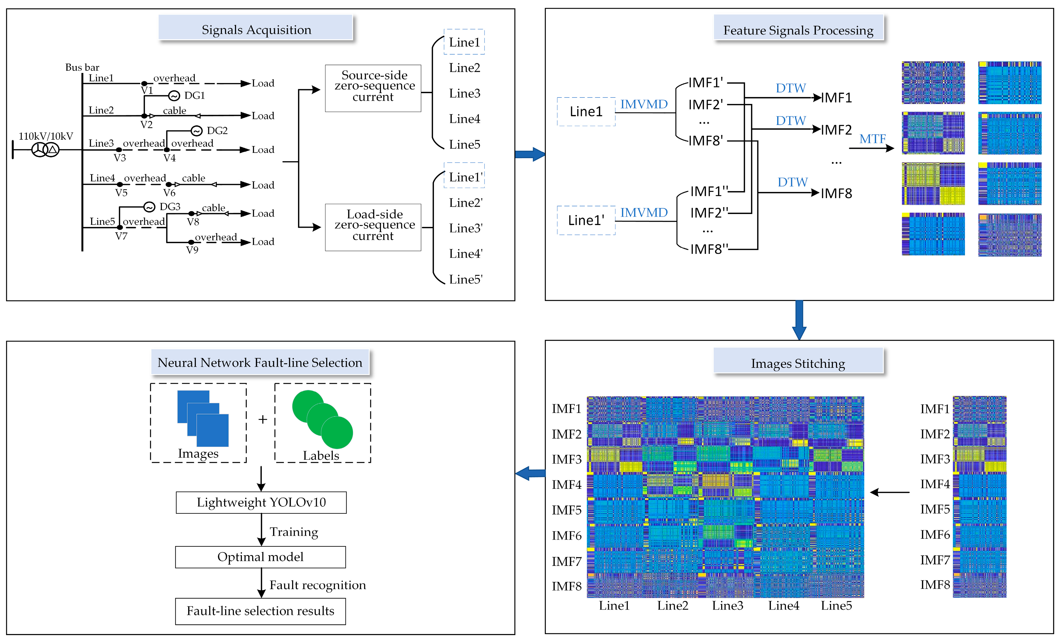
Optimize the MVMD method by using the NGO, and the IMVMD method decomposes the fault characteristic signals, which suppresses modal confusion and pseudo-components to a certain extent;

(2)

Considering the spatio-temporal correlation between the source and load sides of the line, the fault characteristics of the line itself are focused by aligning the source and load signals, which can exclude the influence of load factors on the fault characteristics. The idea of spatio-temporal feature maps is also proposed to visualize the tiny fault features, taking into account the temporal and spatial features of the distribution network;

(3)

Further lightweight improvements are made to YOLOv10 to ensure detection accuracy while reducing the computational overhead so that the model can be better applied to scenarios with limited resources or real-time detection.

The article can be categorized into several sections as follows: Section 1 analyzes the fault mechanism when a single-phase ground fault occurs in an ADN; Section 2 introduces the IMVMD algorithm to decompose the fault signals; Section 3 describes the methods for generating the spatio-temporal feature maps, including the DTW and MTF methods; Section 4 describes the lightweight improvement of YOLOv10 and the process of fault-line selection method; Section 5 shows the results of experiment and comparative analysis.

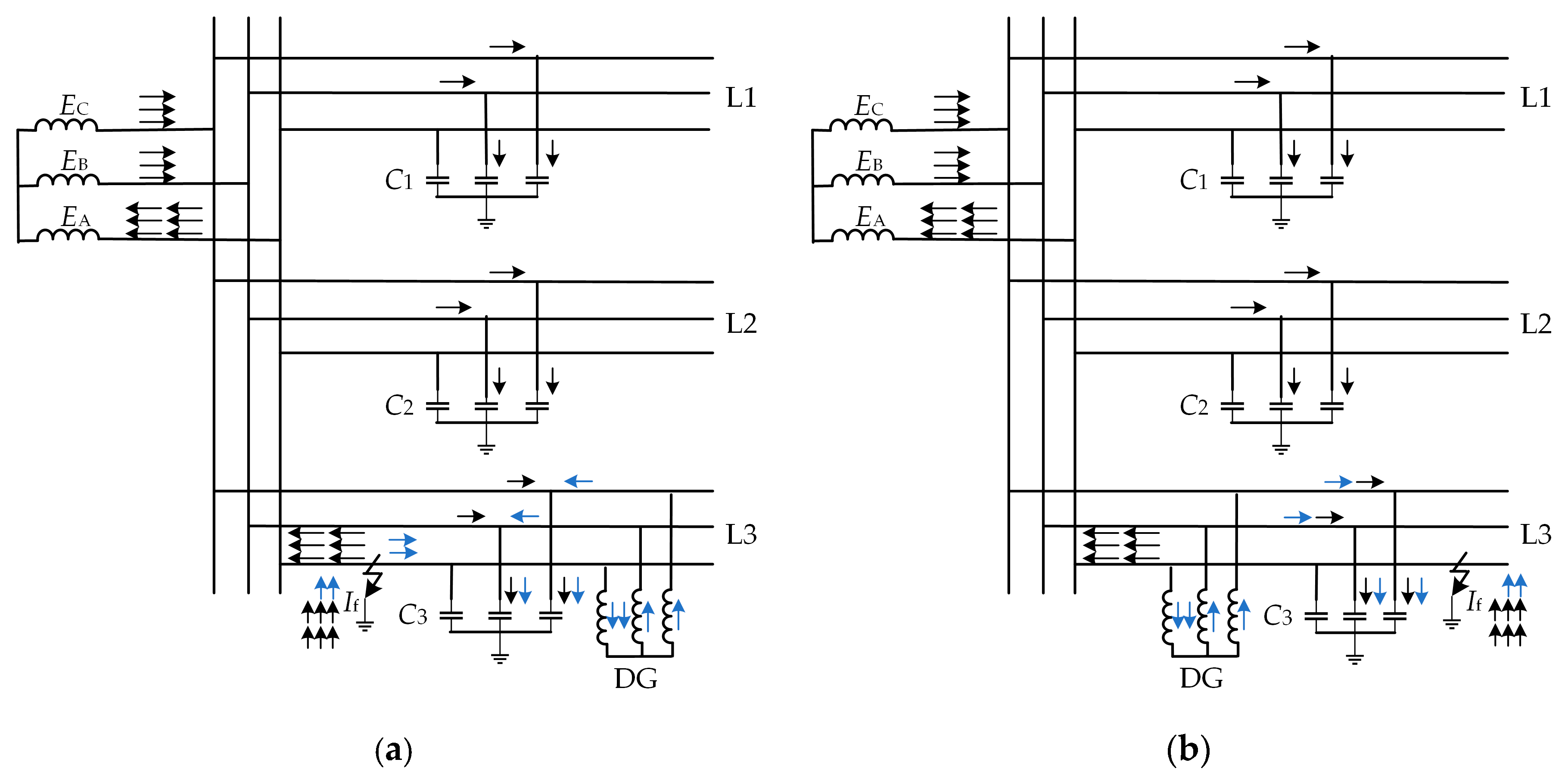
2. Analysis of Ground Fault Mechanism

During single-phase grounding faults in distribution networks, the integration of DGs affects both the magnitude and direction of fault currents within the network. Taking an ungrounded neutral point system as an example, after DG integration, the distribution of ground currents and capacitive currents across various lines is illustrated in Figure 1. When the DG is connected downstream from the fault point, as depicted in Figure 1a, the current component transmitted by the DG and the pre-existing current components near the fault point flow in opposite directions. The zero-sequence currents in non-faulted lines and downstream of the fault point remain as the grounding capacitance currents of lines, with direction from the busbar to the feeder. Upstream of the fault point, the zero-sequence current consists of the sum of zero-sequence currents from non-faulted lines, with direction from the feeder to the busbar. Conversely, when the DG is connected upstream from the fault point, shown in Figure 1b, the characteristics of zero-sequence currents in faulted and non-faulted lines are similar to when the DG is connected downstream from the fault point. Specifically, upstream of the fault point, the zero-sequence current comprises the sum of zero-sequence currents of all normal lines, with opposite polarity to both normal and faulted line zero-sequence currents. Based on the aforementioned analysis, it is evident that DG integration alters the distribution of capacitive currents while preserving the vector relationships of zero-sequence currents between normal and faulted lines. Significant differences in amplitude and phase exist between zero-sequence currents in normal and faulted lines, thereby enabling fault-line selection through characteristic analysis of zero-sequence currents.

3. Method of IMVMD Signal Decomposition

3.1. MVMD Algorithm Based on NGO Optimization

MVMD is an extension of VMD designed for extracting modal components from multivariate time series data, aiming to minimize inter-modal correlations and achieve decomposition by balancing interactions between different components [21]. The decomposition outcome of the MVMD algorithm is influenced by the number of decomposition layers k and the penalty factor α. An excessively high k value can lead to pseudo-components, while too low a value may cause modal confusion. Improper selection of α can affect each component’s decomposition speed and bandwidth. Therefore, the NGO algorithm is utilized to optimize MVMD parameters, selecting optimal k and α values for decomposing zero-sequence currents.

The NGO algorithm replicates the hunting behavior of the northern goshawk, dividing it into two distinct stages: the recognition and attack stage and the chase and escape stage [22]. The northern goshawk population is initialized as shown in Equation (1):

$$X={\left[\begin{array}{l}{X}_1\\ ⋮\\ X_N\end{array}\right]}_{N\times M}=\left[\begin{array}{ccc}{x}_{1,1}& \cdots & x_{1,M}\\ ⋮& \ddots & ⋮\\ x_{N,1}& \cdots & x_{N,M}\end{array}\right]$$

(1)

where X is the northern goshawk population. N is the population size. M is the objective function dimension.

In the first stage, the northern goshawk randomly selects prey and launches an attack, which is a global search and identifies the optimal area within the target range. The mathematical model is shown in Equations (2)–(4):

$$P_i=X_k; i=1, 2, \cdots , N, k=1, 2, \cdots , i-1, i+1, \cdots , N$$

(2)

$$x_{i,j}^{new,P1}=\left\{\begin{array}{l}{x}_{i,j}+r(p_{i,j}-I{x}_{i,j}),F_{p_i}<F_i\\ x_{i,j}+r(I{x}_{i,j}-p_{i,j}),F_{p_i}\ge F_i\end{array}\right.$$

(3)

$$X_i=\left\{\begin{array}{l}{X}_i^{new,P1},F_i^{new,P1}<F_i\\ X_i,F_i^{new,P1}\ge F_i\end{array}\right.$$

(4)

where P_i is the position of the ith northern goshawk’s prey, and F_Pi is the value of its objective function. X_i is the position of the ith northern goshawk, and F_i is the value of its objective function. $x_{i,j}^{new,P1}$ is the new position of the ith northern goshawk in the j-dimension of the first stage, and $F_i^{new,P1}$ is the objective function value corresponding to the new position; r is the number of random numbers in the interval (1, N). I is the random number 1 or 2.

In the second stage, the prey tries to escape, and the northern goshawk continues to pursue and complete the capture of the prey. In this stage, the search space is searched locally to find the optimal solution, and the mathematical model is shown in Equations (5)–(7):

$$x_{i,j}^{new,P2}=x_{i,j}+R(2r-1)x_{i,j}$$

(5)

$$R=0.02(1-{\displaystyle \frac{t}{T}})$$

(6)

$$X_i=\left\{\begin{array}{l}{X}_i^{new,P2},F_i^{new,P2}<F_i\\ X_i,F_i^{new,P2}\ge F_i\end{array}\right.$$

(7)

where $x_{i,j}^{new,P2}$ is the new position of the ith northern goshawk in the second stage in j-dimension, and $F_i^{new,P2}$ is the value of its objective function. R is the radius of the pursuit range. t is the number of iterations. T is the maximum number of iterations.

In the optimization of MVMD using the NGO algorithm, the minimum envelope entropy value is adopted as the objective function, and the parameter optimization process is realized by finding the global minimum envelope entropy as well as the corresponding optimal values [k, α]. In Figure 2, the specific process is illustrated.

Considering the performance and speed of the optimization algorithm, parameters are set as k ∈ [3, 8] and α ∈ [600, 2000], with a population size of 30 and a maximum iteration number of 20. Since other parameters have relatively minor effects on MVMD decomposition results, they are set based on empirical values. Noise tolerance tau = 0, initial center frequency init = 1, direct current component DC = 0, and convergence tolerance criterion tol = 1 × 10⁻⁷. Utilizing the IMVMD optimization algorithm effectively separates the frequency components of zero-sequence currents and suppresses mode mixing. To eliminate noise components, components with permutation entropy greater than 0.6 are identified and removed as noise signals [23], thereby providing effective denoising of zero-sequence current signals and enhancing noise resistance capabilities of fault-line selection.

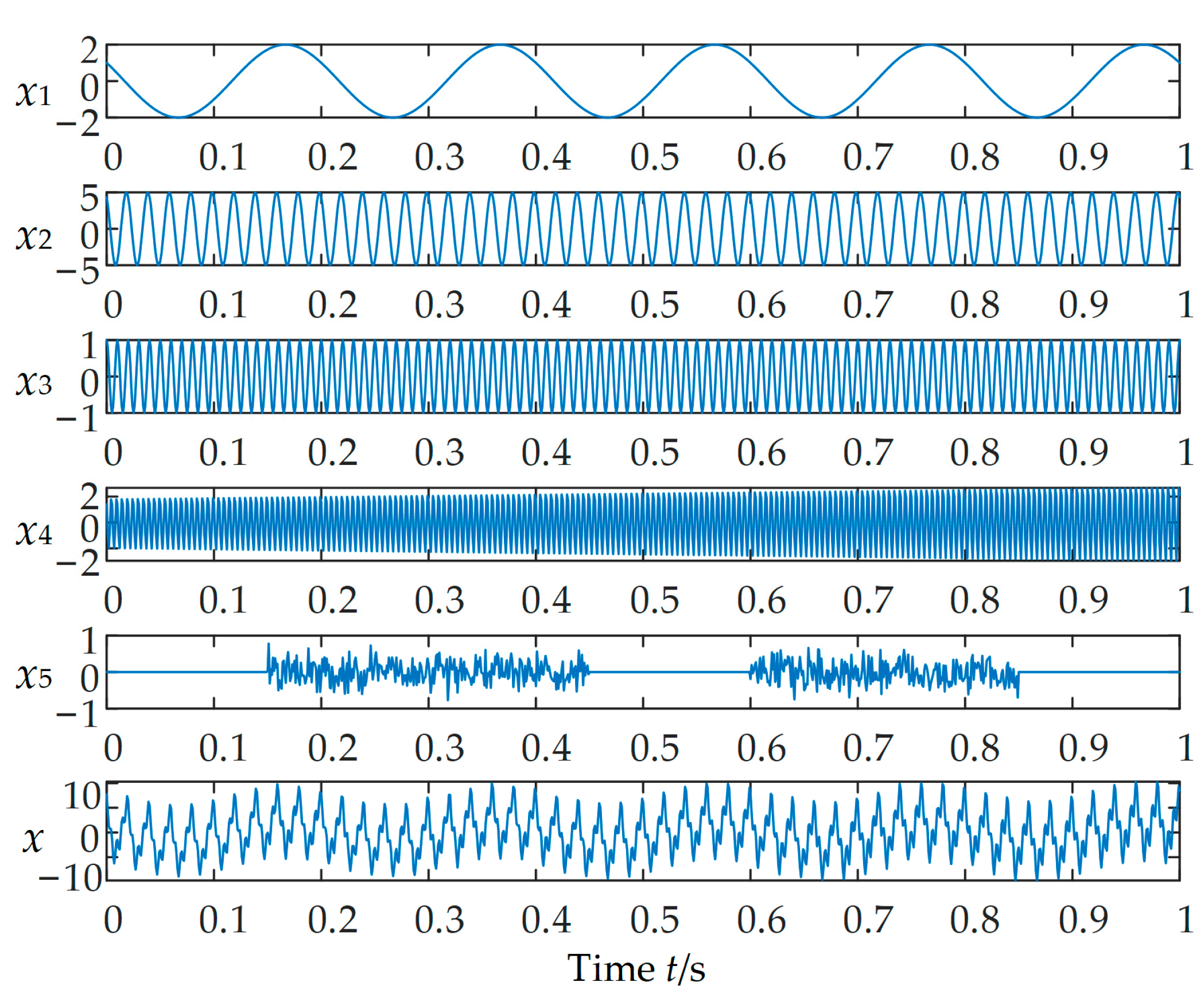
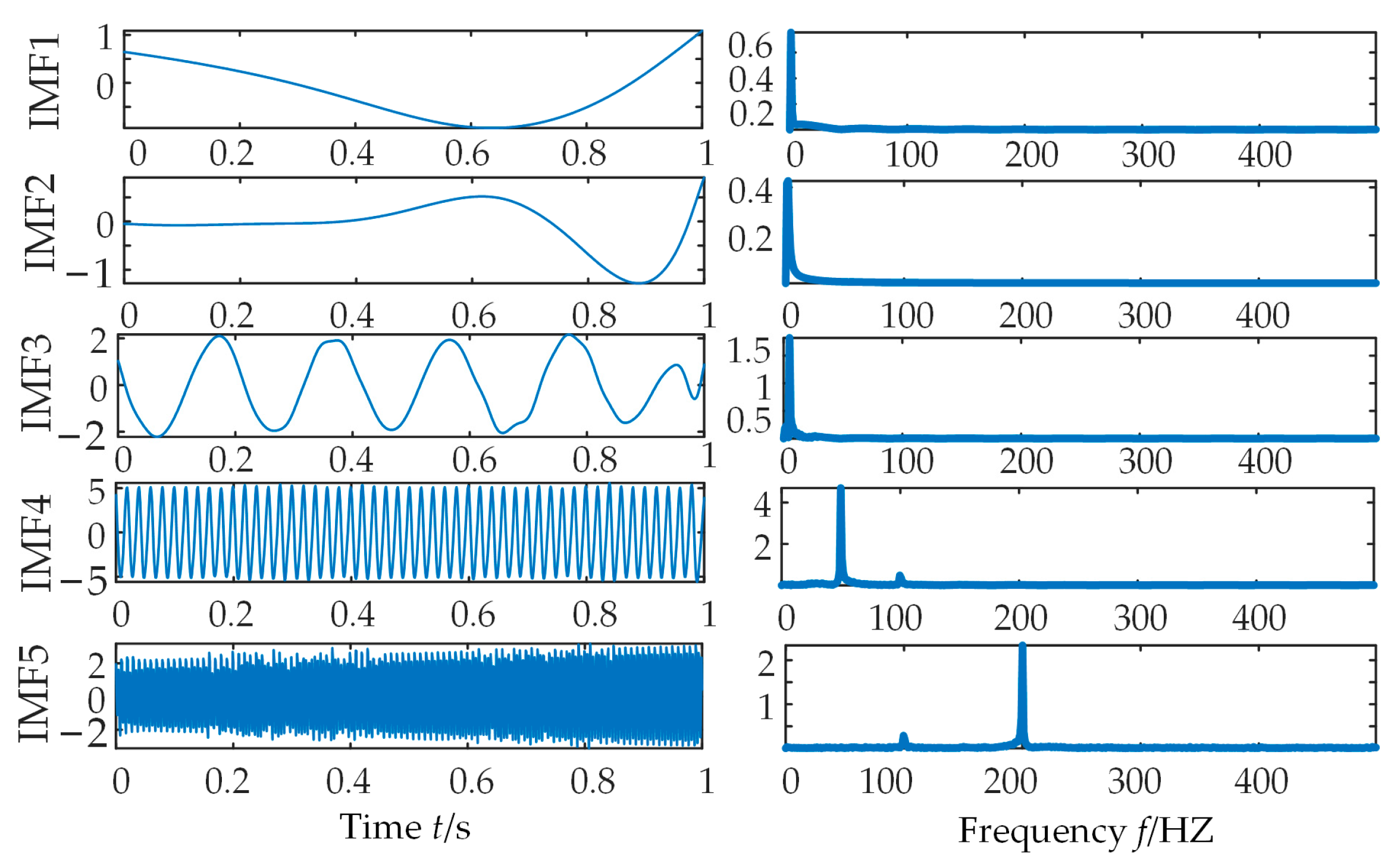
3.2. Analysis of Decomposed Simulated Signals

To illustrate the performance of the IMVMD algorithm, simulated signals are utilized for analysis. The original simulation signal x consists of x₁, x₂, x₃, x_4, and a random noise sequence x₅, and the expression is shown in Equation (8). The frequency of sampling is 1 kHZ, and the time of sampling is 1 s, as depicted in Figure 3.

$$\left\{\begin{array}{l}{x}_1=2\cos (2\pi \times 5t+\pi /3)\hfill \\ x_2=5\cos (2\pi \times 50t+\pi /6)\hfill \\ x_3=\cos (2\pi \times 100t)\hfill \\ x_4=(t+2)\cos (2\pi \times 200t+\pi /4)\hfill \\ \begin{array}{l}{x}_5=[zeros(1,150), 0.3randn(1,300), zeros(1,150), 0.3randn(1,250), zeros(1,150)]\\ x=x_1+x_2+x_3+x_4+x_5\end{array}\hfill \end{array}\right.$$

(8)

The original signal x is decomposed using the empirical mode decomposition (EMD). The results of decomposition are depicted in Figure 4. As illustrated, EMD divides original signal x into five IMFs. Still, modal mixing occurs in IMF1, IMF2, and IMF3, and the decomposition is incomplete, and there are pseudo-components.

The original simulated signal is decomposed by the IMVMD optimization algorithm, as shown in Figure 5. The IMVMD algorithm can effectively separate the various frequency components of the original signal as well as the noise part without modal aliasing, and there is no problem with incomplete decomposition and pseudo-components.

4. Methods for Spatio-Temporal Feature Map Generation

4.1. Alignment Methodology of Source and Load Based on DTW

The DTW algorithm is a method for computing similarity between two discrete time series. By finding the optimal path that minimizes the sum of the dynamic regularization distances and minimizing the cumulative distance between the two, the optimal alignment path and optimal solution for two series of different lengths are obtained [24].

The number of IMF components is K for both the source and load sides of zero-sequence current signals. The time series of the kth IMF component from the source and load sides are denoted as A = {a₁, a₂, …, a_m} and B = {b₁, b₂, …, b_n}, respectively. The distance between any two points is represented by the Euclidean distance d(a_i, b_j) = ∣a_{i −} b_j∣, and an m × n distance matrix D for sequences A and B is constructed as shown in Equation (9):

$$D=\left[\begin{array}{cccc}d(a_1,b_1)& d(a_2,b_1)& \cdots & d(a_m,b_1)\\ d(a_1,b_2)& d(a_2,b_2)& ⋮& d(a_m,b_2)\\ \cdots & \cdots & \cdots & \cdots \\ d(a_1,b_n)& d(a_2,b_n)& \cdots & d(a_m,b_n)\end{array}\right]$$

(9)

The DTW algorithm identifies the optimal alignment path W by minimizing the sum of distances along the path, as expressed in Equation (10):

$$\left\{\begin{array}{l}W=\left\{w_1,\dots ,w_k,\dots ,w_l\right\}\\ w_k=({\alpha }_k,{\beta }_k)\\ \max (m,n)\le l\le m+n-1,1\le {\alpha }_k\le m,1\le {\beta }_k\le n\end{array}\right.$$

(10)

where (α_k, β_k) denotes the α_kth value in sequence A and its corresponding β_kth value in sequence B.

The optimal path W is determined using dynamic programming principles, adhering to continuity and monotonicity constraints, with only three kinds of cumulative directions for each distance element of the path: (i, j − 1), (i − 1, j) or (i − 1, j − 1). The global minimum cumulative distance matrix D_c is recursively defined by Equation (11):

$$\left\{\begin{array}{l}{D}_{\mathrm{c}}(1,1)=d(a_1,b_1)\\ D_{\mathrm{c}}(i,1)=d(a_1,b_1)+D_{\mathrm{c}}(i-1,1)\\ D_{\mathrm{c}}(1,j)=d(a_1,b_1)+D_{\mathrm{c}}(1,j-1)\\ D_{\mathrm{c}}(i,j)=d(a_i,b_j)+\min [D_{\mathrm{c}}(i,j-1),D_{\mathrm{c}}(i-1,j),D_{\mathrm{c}}(i-1,j-1)]\end{array}\right.$$

(11)

where i > 1 and j > 1.

The shortest path method computes the optimal path between the starting point d(a₁, b₁) and the ending point d(a_m, b_n), yielding the optimal alignment path W. The elements corresponding to the optimal alignment path W in distance matrix D constitute the 1D time series W_D = {D(α₁, β₁), …, D(α_k, β_k), …, D(α_l, β_l)}.

4.2. Generation Methodology of MTF Images

MTF is an image encoding method based on Markov transition probabilities [25]. It treats the 1D time series of the optimal alignment path as a Markov process to construct a Markov transition field, enabling the transformation of 1D sequences into 2D images. This approach facilitates the visualization of fault information for convolutional neural networks.

For the 1D time series X = (x_t, t = 1, 2, …, T). The data are partitioned into Q quantiles based on their distribution characteristics, with each quantile q_j (j ∈ [1, Q]) representing a respective bin. The values x_i of sequence X are mapped to their corresponding quantiles q_j. Transition probabilities between these quantiles q_j are computed using principles of first-order Markov chains to construct a Q × Q transition matrix W, as shown in Equation (12):

$$W=\left[\begin{array}{cccc}{w}_{11}& w_{12}& \cdots & w_{1Q}\\ w_{21}& w_{22}& \cdots & w_{2Q}\\ ⋮& ⋮& \ddots & ⋮\\ w_{Q1}& w_{Q1}& \cdots & w_{QQ}\end{array}\right]$$

(12)

where w_ij = P(x_t ∈ q_j | x_{t − 1} ∈ q_i) represents the one-step transition probability from quantile q_i to quantile q_j.

To preserve both the temporal and positional information of sequence X, the probability information from the transition matrix W is extended along the time axis to form the Markov transition field matrix M, as shown in Equation (13):

$$M=\left[\begin{array}{ccc}{w}_{ij}|x_1\in q_i,x_1\in q_j& \cdots & w_{ij}|x_1\in q_i,x_T\in q_j\\ ⋮& \ddots & ⋮\\ w_{ij}|x_T\in q_i,x_1\in q_j& \cdots & w_{ij}|x_T\in q_i,x_T\in q_j\end{array}\right]$$

(13)

The elements of matrix M are treated as pixels, thus transforming into a 2D image. The resulting MTF image encapsulates both the temporal characteristics and state transition properties of the original signal, facilitating feature visualization. The MTF image generation process is illustrated in Figure 6.

5. Method of Fault-Line Selection Based on Lightweight YOLOv10 Network

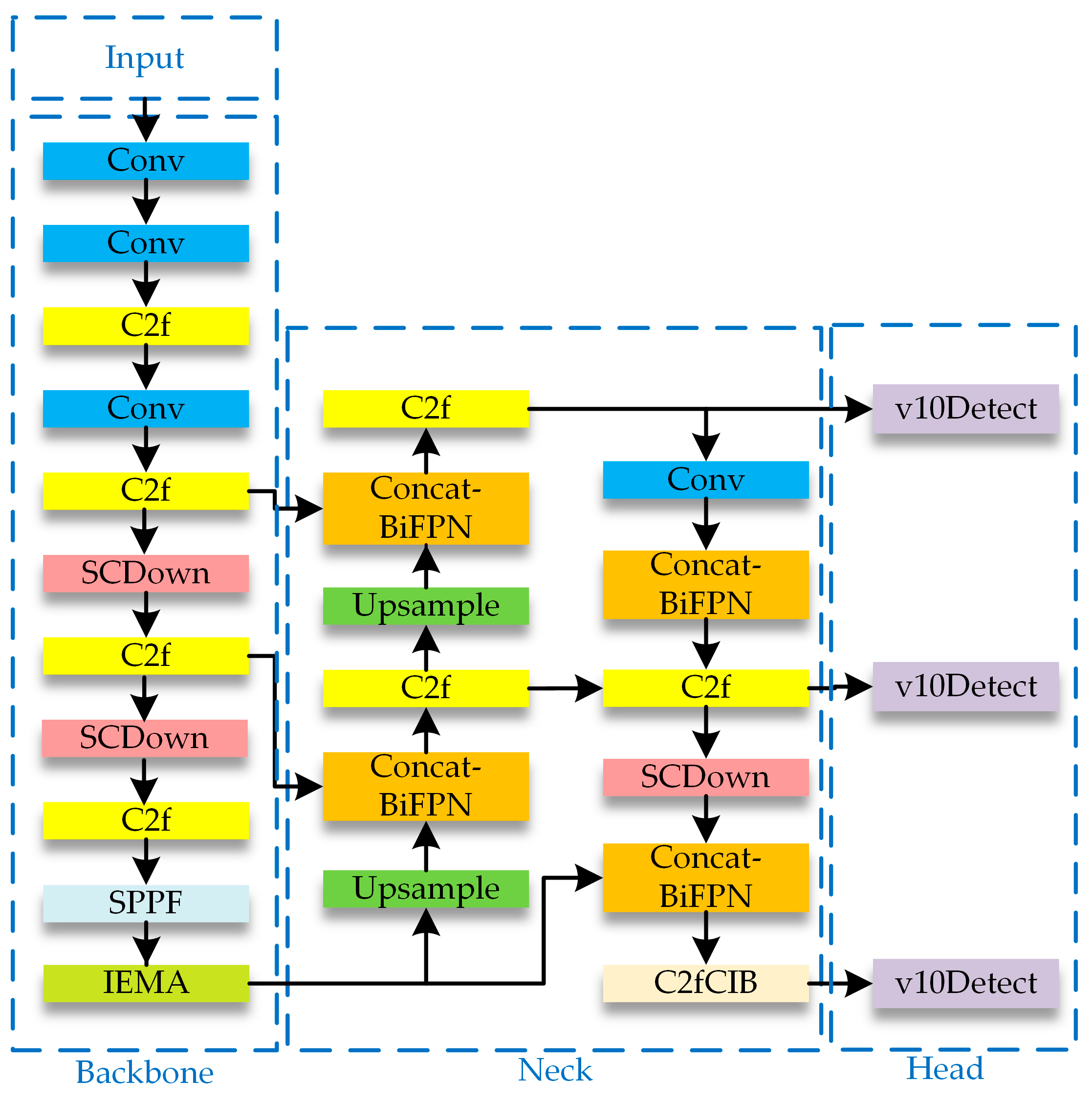
5.1. Lightweight YOLOv10 Neural Network Model

YOLOv10 represents the latest iteration of the YOLO model, incorporating new functionalities and innovative methods to enhance performance and efficiency significantly. Notably, it introduces the concept of Consistent Dual Assignments without Non-Maximum Suppression (NMS) training, which improves performance while reducing inference latency [26]. Furthermore, comprehensive optimizations have been applied to various components of YOLO from both efficiency and accuracy perspectives. The YOLOv10 network introduces several novel structures, including Compact Inverted Block (CIB), Spatial-channel Decoupled Down-sampling (SCDown), Partial Self-Attention (PSA), and detection heads. These innovations collectively contribute to its enhanced capabilities in real-time object detection tasks. To further enhance YOLOv10 lightweight capabilities without compromising accuracy, the following improvements have been proposed. These optimizations aim to reduce computational overhead while preserving model performance. The network architecture of lightweight YOLOv10 is illustrated in Figure 7.

The Efficient Multi-Scale Attention (EMA) module is used to replace the Multi-Head Self-Attention (MHSA) module of PSA in YOLOv10 to form the new module, which is an improved EMA (IEMA). The IEMA module reshapes the channel dimension so that the spatial semantic features are uniformly distributed, adopts the idea of parallel sub-networks, captures both spatial and channel information through cross-dimensional information interaction, and adaptively adjusts the weight of each channel using the current context information to improve the attention to the local detail information and at the same time reduces the computational overhead [27].

The Bi-directional Feature Pyramid Network (BiFPN), an enhancement of the PAN-FPN structure in YOLOv10, introduces bi-directional connections between adjacent levels of the feature pyramid. This design facilitates interaction and fusion of multi-scale features, effectively removing nodes with weaker fusion capabilities to improve information transmission efficiency and achieve further lightweight [28]. Substituting the PAN-FPN structure with BiFPN in YOLOv10 preserves model accuracy while enhancing performance and efficiency.

5.2. Flow of Fault-Line Selection Method

Considering zero-sequence currents’ time–frequency characteristics and spatio-temporal correlation between sources and loads and aiming to exploit deep features of fault signals fully, this paper proposes a fault-line selection method for ADNs based on NGO-MVMD and a lightweight YOLOv10 network. The zero-sequence currents at source and load ends are taken as raw signals and decomposed via NGO-MVMD to obtain IMFs rich in time–frequency characteristics. Using DTW, the IMFs of corresponding layers from source and load ends are aligned to preserve the spatio-temporal characteristics of fault signals, thereby mitigating the influence of practical factors like load phase imbalance on fault feature extraction and enhancing anti-interference capability. The alignment path is treated as a 1D time series and transformed into a 2D spatial image using MTF, enabling visualization of otherwise imperceptible information and leveraging neural networks’ advantages in image recognition. To balance the time–frequency and spatial characteristics of fault signals while minimizing redundancy in training datasets, MTF images are concatenated into spatio-temporal feature maps and fed into the lightweight YOLOv10 network for deep fault information mining, ensuring accurate and efficient fault identification. The fault-line selection process for single-phase-to-ground faults in ADNs is illustrated in Figure 8. The specific steps are outlined as follows:

Step 1: Construct a simulation model of the distribution network, setting fault nodes on each line and varying fault parameters such as phase, distance, initial phase angle, and grounding resistance to collect zero-sequence currents at source and load ends as raw data for each line.

Step 2: Optimize the parameters of MVMD by NGO, decompose the collected source zero-sequence currents, and load zero-sequence currents using IMVMD. Each zero-sequence current signal can be optimally decomposed to obtain K IMFs.

Step 3: Align the IMFs from source and load ends in ascending order of frequency using DTW, calculating the optimal alignment path of time series for the kth IMF (k = 1,2,…, K) of both source and load ends, and transform the 1D time series into a 2D spatial images using MTF.

Step 4: Vertically concatenate all IMF images of a single line to form a spatio-temporal feature subgraph of the source-load zero-sequence current signals for that line. Horizontally concatenate these feature subgraphs from all lines in the ADN to construct the spatio-temporal feature map of the overall network.

Step 5: Utilize label software to annotate all spatio-temporal feature maps, delineating fault lines with bounding boxes to generate label files readable by the YOLOv10 network. These label files consist of custom annotations specifying fault-line identifiers and rectangular box coordinates. Input the images and labels into the lightweight YOLOv10 network for training, generating model files applicable to fault-line selection in ADNs.

6. Experimental Results and Analysis

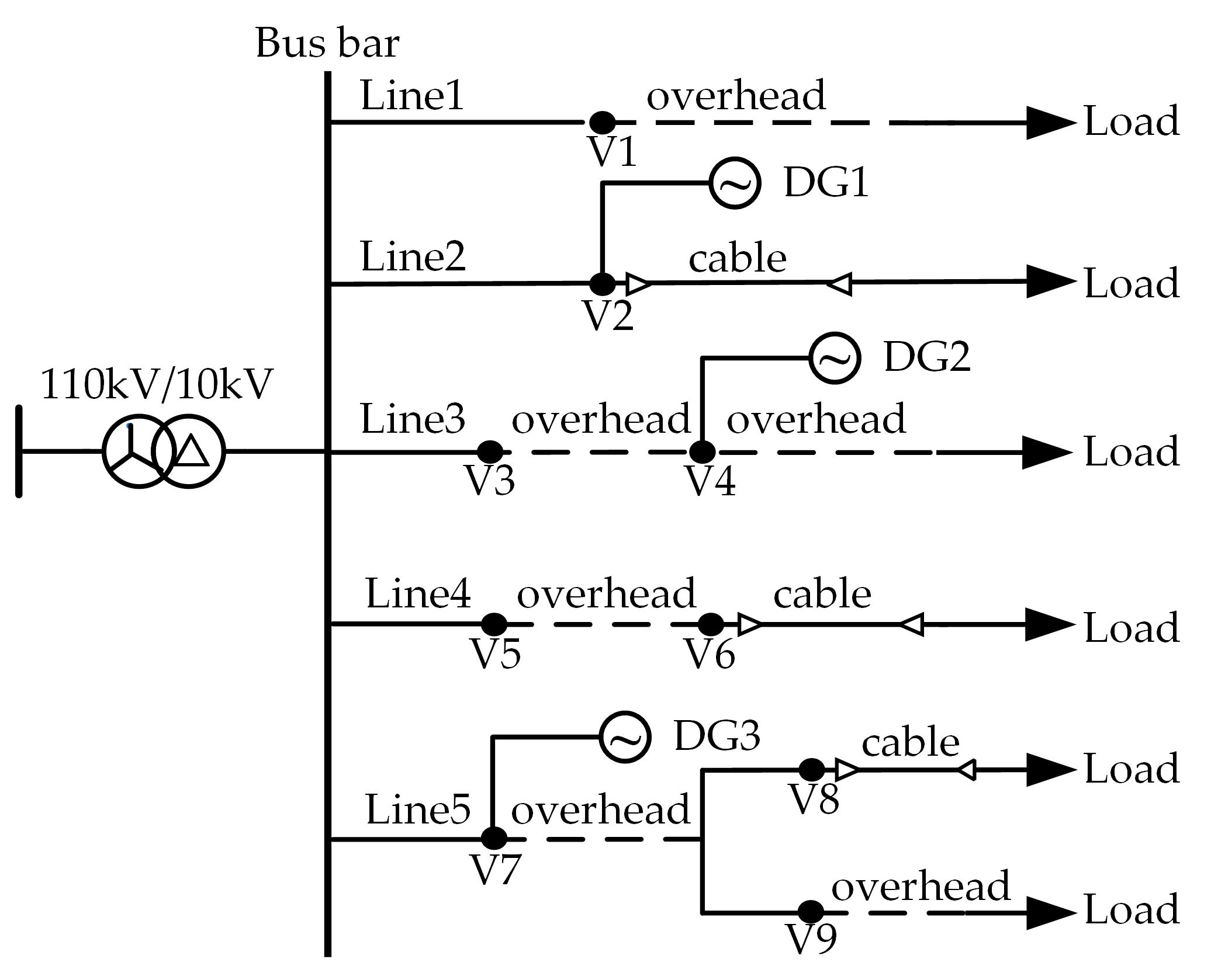
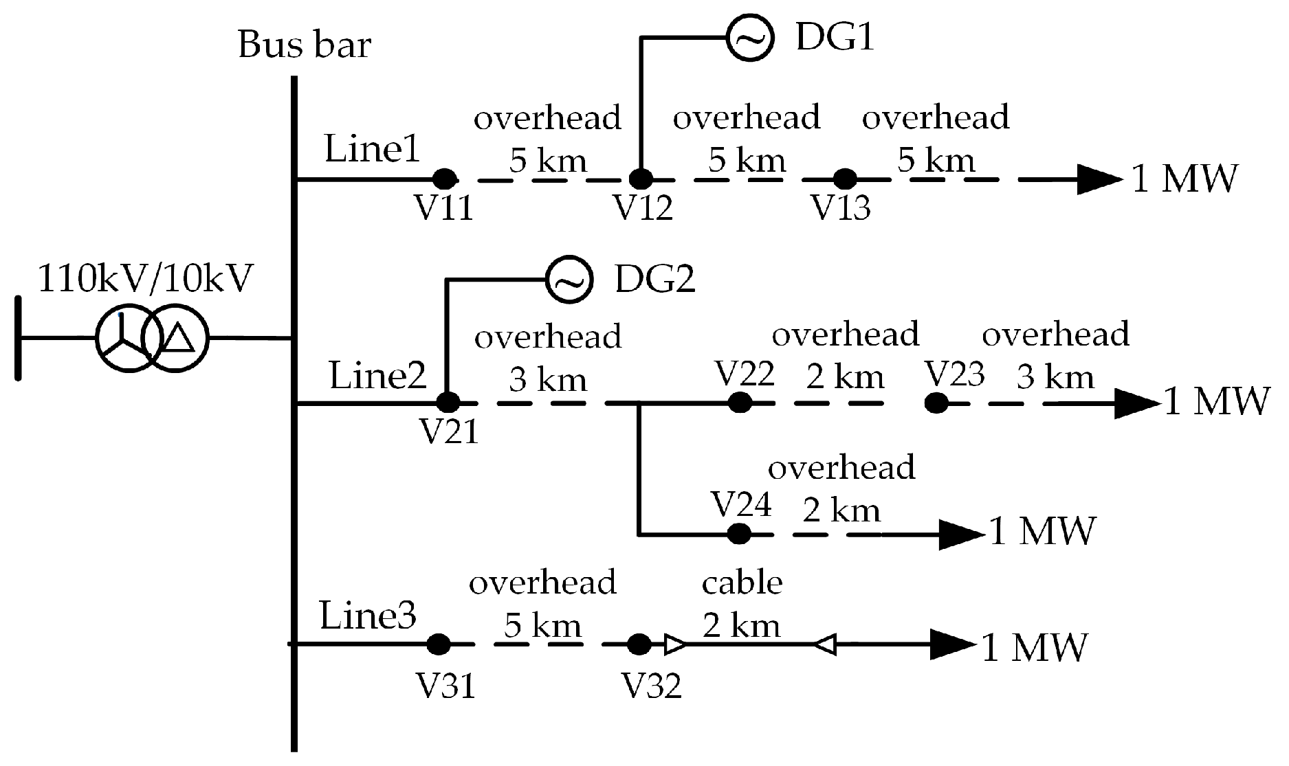
6.1. Active Distribution Network Model

The 110kV/10kV radial ADN model based on MATLABR2022b/SIMULINK is established, adopting the neutral ungrounded mode. The network topology is shown in Figure 9. It consists of 5 lines, of which line 1 is an overhead line with a length of 5 km, line 2 is a pure cable line with a length of 4 km, line 3 is two overhead lines with lengths of 3 km and 4 km, line 4 consists of a pure cable line with a length of 5 km and an overhead line with a length of 3 km, line 5 consists of an overhead line with a length of 4 km and two pure cable lines with lengths of 3 km and 4 km. Line 2, line 3, and line 5 are connected to the DGs, and the line parameters are shown in

Table 2. Parameters of the simulated line.

Circuit Type	Resistance/(Ω·km−1)		Inductance/(mH·km−1)		Grounding Capacitance/(μF·km−1)
	Positive Phase	Zero Phase	Positive Phase	Zero Phase	Positive Phase	Zero Phase
Overhead Line	0.178	0.25	1.21	5.54	0.015	0.012
Cable Line	0.27	2.7	0.255	1.02	0.339	0.28

.

In order to simulate the operation of the ADN in the actual working situation, the faulty phases of different lines, the initial phase angle of the fault, the faulty distance, and the fault grounding resistance are set, respectively. The sampling frequency is 12.8 kHz, the system operation time is 0.1 s, and a single-phase ground fault is triggered after 0.02 s of normal operation. The zero-sequence current signals of one cycle before the fault and four cycles after the fault are collected as raw data. Faults are set sequentially from line 1 to line 5, with fault phases selected between phase A, phase B, and phase C. The initial phase angles of the faults are 0°, 30°, 60°, 90°, 120°, and 150° in turn, and considering the difference in the results of the selection of high and low resistance of the grounding resistance, the low resistance is set to start from 0 Ω to 50 Ω, and the high resistance is set to start at 100 Ω and increase in 300 Ω increments up to 1 300 Ω. The faulty distance begins at 1 km from the starting point and sets a fault point every 1 km to 1 km from the end of the line. A total of 6006 sets of fault feature images are collected. Based on the proportion of different fault types for each line, the data are randomly divided into a training set, validation set, and test set in an 8:1:1 ratio, where 4806 images are used as a training set, 600 images as a validation set, and 600 images as a test set.

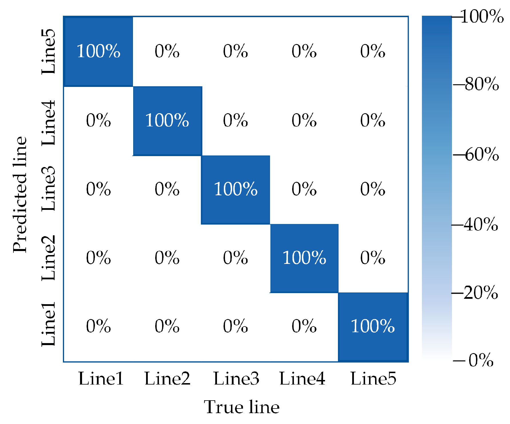
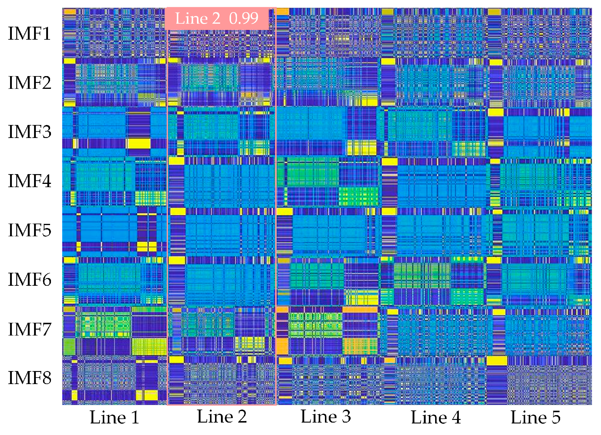
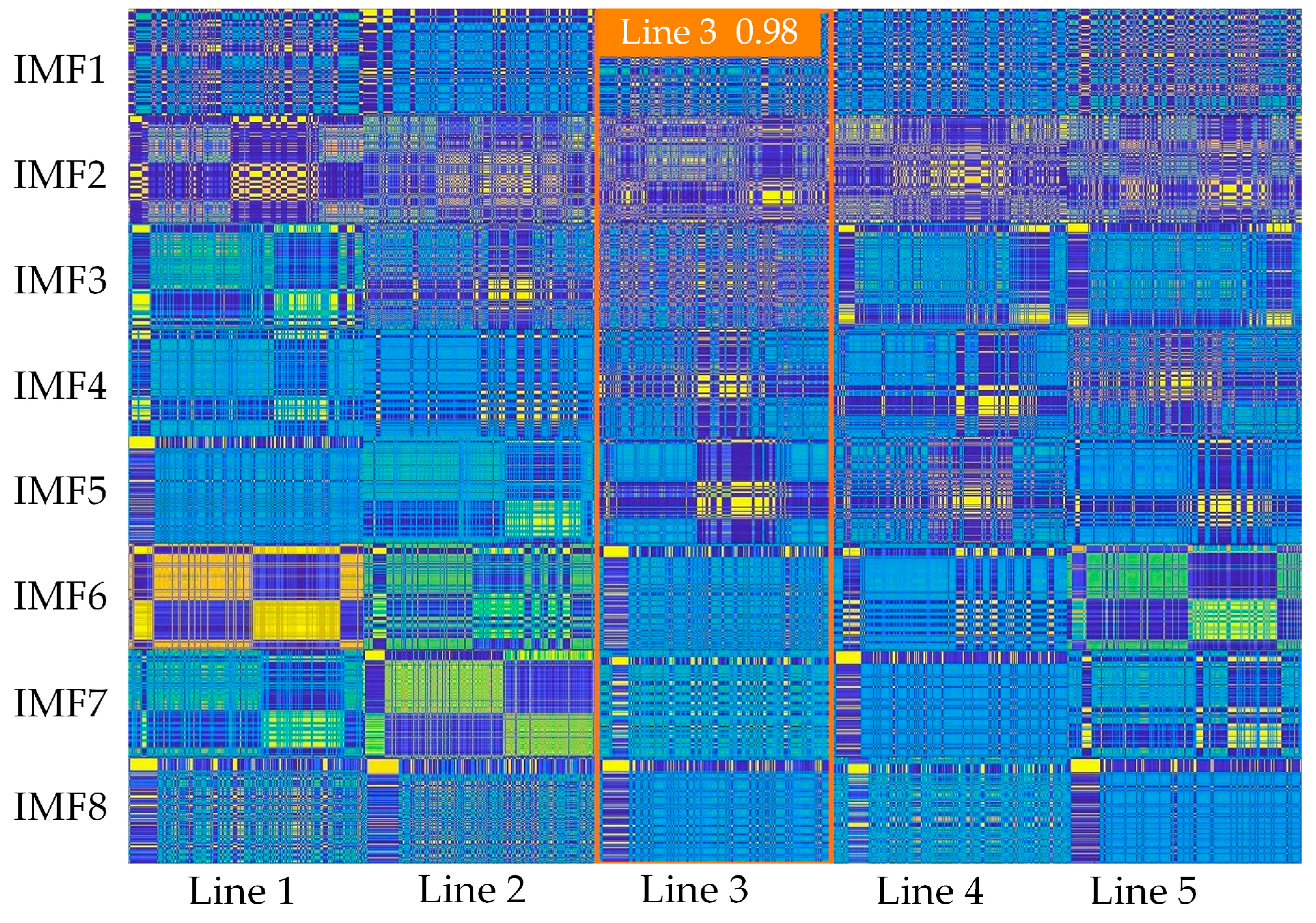
6.2. Analysis of Line Selection Results

After 50 rounds of training using the lightweight YOLOv10 model, the model has gradually converged, and its precision, recall, and mean average precision (mAP) values are steadily stabilized. The number of training rounds is set to 100 rounds, as shown in Figure 10. As the number of training epochs increases, the target detection loss (box_loss), classification loss (cls_loss), and dynamic feature loss (dfl_loss) for both the training set and validation set gradually decrease and approach zero. The loss value of the training set decreases, and the loss value of the validation set also decreases, which indicates that the model has no overfitting phenomenon. The line selection precision gradually increases and finally stabilizes at 99.88%, the recall converges to 100%, and the mAP converges to 99.5%. Figure 11 shows the confusion matrix obtained from the validation analysis for the validation set, from which it can be seen that for the validation set fault samples, the fault-line selection method achieves 100% line selection accuracy for each faulty line.

Perform fault-line selection of the test set using the optimal model obtained from training. The target detection outputs the result as an image of the fault line labeled by a rectangular box. Take line 2 and line 3 ground fault as an example. When a phase A ground fault occurs at 1 km from the bus in line 2, the grounding resistance is set as 1500 Ω. Figure 12 shows the fault-line selection result. When the number of DGs is increased, a phase C ground fault occurs at 3 km from the bus in line 3, and the grounding resistance is set as 500 Ω. Figure 13 shows the fault-line selection result. From the line selection results, it can be seen that the method can not only accurately select the line for high-resistance ground faults but also ensure the line selection accuracy in the case of changing the penetration rate of DGs.

6.3. Comparison and Verification

In order to verify the effectiveness and accuracy of the fault-line selection method in this paper, comparative experiments are conducted on the performance and improvement results of the lightweight YOLOv10 network. The interference immunity, high-resistance grounding, and two-point fault detection capabilities are also compared and verified using a certain number of sample data. And the effectiveness of the method in practical applications is also verified on a dynamic real-time simulation platform.

6.3.1. Comparison of Different Neural Networks

To validate the advantages of the lightweight YOLOv10, YOLOv8, YOLOv10, and an enhanced lightweight version of YOLOv10 were trained on the same dataset. A comparison was made among the three networks based on parameters, computational complexity, weight file sizes, and accuracy.

According to

Table 3. Comparative results before and after improvement.

Model	Parameters/M	FLOPs/G	Weights File/MB	Training Rounds	Accuracy/%
YOLOv8	3.0	8.1	6.2	150	99.85
YOLOv10	2.7	8.2	5.8	100	99.86
Lightweight YOLOv10	2.6	8.2	5.4	100	99.88

, compared to YOLOv8, YOLOv10 exhibits significantly reduced parameter count, along with improved model convergence speed and accuracy of detection. The improved lightweight YOLOv10, built upon the original YOLOv10 framework, undergoes further optimizations without sacrificing accuracy, thereby reducing parameters and computational overhead. This effectively minimizes weight file sizes, enabling the model to suit resource-constrained environments better.

6.3.2. Verification of Noise Resistance

Under the actual working conditions, the raw signals collected from the ADN contain some noise. To verify the noise immunity of the method, different methods are used.

Method 1: The zero-sequence currents at both ends of the source and load are directly computed using DTW and then converted into images using MTF.

Method 2: The zero-sequence currents at both ends of the source and load are decomposed using EMD. The aligned paths of corresponding components are calculated via DTW and subsequently transformed into images using MTF.

Method of This Paper: The source-load zero-sequence currents are decomposed using IMVMD. DTW calculates the aligned paths of corresponding components, which are then transformed into images using MTF.

The feature images obtained by the above three methods are trained and tested with the lightweight YOLOv10 network, and the results are shown in

Table 4. Comparison and analysis of different methods.

Faulty Line	Samples Size	Accuracy/%
		Method 1	Method 2	This Paper
Line 1	200	91.21	95.67	99.99
Line 2	300	93.18	95.26	99.97
Line 3	500	92.23	94.28	99.98
Line 4	600	90.33	94.42	99.98
Line 5	800	90.15	94.39	99.99

.

Based on the table, it is evident that utilizing IMVMD to decompose zero-sequence currents, aligning IMFs between source and load using DWT, and then transforming them into images via MTF effectively separates and filters out noise. This significantly improves the accuracy of fault-line selection, demonstrating the robust noise resistance capability of the method proposed in this paper.

To further verify that the proposed method has a certain anti-noise performance, Gaussian white noise with different signal-to-noise ratios is added to the original signal.

Comparison of line selection under the same working conditions is carried out for the polarity comparison method and amplitude comparison method in the classical methods, as well as for the SVM, CNN, and lightweight YOLOv10 in the data-driven methods, respectively. The fault-line selection accuracy of different methods with different signal-to-noise ratios (SNRs) is shown in

Table 5. Comparison of line selection accuracy under different SNRs.

SNR/dB	Number of Samples	Accuracy/%
		Polarity Comparison	Amplitude Comparison	SVM	CNN	Lightweight YOLOv10
50	435	93.21	81.56	88.33	96.82	100
40	435	90.66	75.88	87.50	93.56	99.98
30	435	87.20	69.31	86.67	89.50	99.86
20	435	84.51	57.62	75.00	81.29	99.64

.

As can be seen from the table, when the original signal contains 20 dB to 50 dB of noise, with the increase in noise percentage, the other methods are more disturbed by the noise, while the proposed method can still maintain high fault-line selection accuracy. The lightweight YOLOv10 network has a certain filtering effect compared with other networks, which shows that the method in the paper has a certain anti-noise performance in fault-line selection in the ADN.

6.3.3. Comparative Verification of High-Impedance Faults

When a high-impedance fault occurs, the characteristics of signal fault are even weaker. This situation may lead to a decrease in the accuracy of fault-line selection. The method proposed in this paper retains the spatio-temporal characteristics of fault information by visualizing the fault features and fully exploits the deep features by using neural networks, and the method still maintains high accuracy under high-impedance faults. Comparing the method of this article with reference [12] and reference [15], setting the resistance value of high-resistance grounding fault from 2000 Ω to 5000 Ω, the experimental results are shown in

Table 6. Comparison of high-resistance grounding fault-line selection results.

Resistance/Ω	Faulty Line	Results
		Ref. [12]	Ref. [15]	This Article
2000	Line 1	Line 1	Line 1	Line 1
	Line 2	Line 2	Line 2	Line 2
2500	Line 3	Line 3	Line 3	Line 3
	Line 4	Line 4	Line 4	Line 4
3000	Line 5	Line 5	Line 3	Line 5
	Line 1	Line 1	Line 1	Line 1
4000	Line 2	Line 2	Line 2	Line 2
	Line 3	Line 4	Line 4	Line 3
5000	Line 4	Line 4	Line 3	Line 4
	Line 5	Line 3	Line 4	Line 5

.

As can be seen from the table, the value of the grounding resistance increases, reference [12] and reference [15] suffer from misjudgment under high-impedance faults, while this article is still able to correctly detect the faulted line in the case of high-impedance faults and maintains a high accuracy rate.

6.3.4. Comparative Verification of Two-Point Same-Phase Grounding Fault

When a complex fault occurs in which two points are connected to the ground in the same phase, the difficulty of fault-line selection is increased due to the fact that the shunt results in much smaller zero-sequence currents of the faulted line. The method of this paper is compared with the reference [12] and reference [15] by setting up a two-point same-phase ground fault, and the comparison results are shown in

Table 7. Comparison of the results of line selection for two-point same-phase ground faults.

Fault Line	Type of Fault	Fault-Line Selection Results
		Ref. [12]	Ref. [15]	This Paper
Line 1	AG	Line 1	Line 1	Line 1
Line 2		Line 2		Line 2
Line 2	BG	Unselected	Line 5	Line 2
Line 3				Line 3
Line 4	CG	Line 5	Unselected	Line 4
Line 5				Line 5

.

According to the table, methods described in references [10] and [14] exhibit issues of omission and misjudgment, failing to correctly identify both faulty lines simultaneously. In contrast, our approach accurately detects faults in both lines without any false alarms or missed detections. Therefore, our method maintains high accuracy in complex fault identification scenarios involving multiple faults.

6.3.5. Dynamic Mold Experiment

In order to better simulate the single-phase ground fault-line selection scenario in the actual ADN and verify the effectiveness of the proposed method in practical applications, the dynamic simulation fault diagnosis experimental platform shown in Figure 14 is used to experimentally verify the method in this paper. Utilizing MATLAB/Simulink, the same model of simulation topology as the dynamic simulation fault diagnosis experimental platform has been constructed, as shown in Figure 15. This topology model includes three lines and two DGs. The simulation model is utilized to collect data and train the model. The dynamic simulation fault diagnosis experimental platform collects actual data and uses them to test the line selection accuracy of the model and verify the reliability of the method proposed in this paper. The results are presented in

Table 8. Fault-line selection results under the conditions of the dynamic simulation fault diagnosis experimental platform.

Fault Type	Fault Line	Fault Point	Transition Resistance/Ω	Fault Close Angle	Fault Location Result
AG	Line 1	V11	0	0°	Line 1
BG	Line 1	V12	100	30°	Line 1
CG	Line 1	V13	800	60°	Line 1
AG	Line 2	V21	400	60°	Line 2
BG	Line 2	V22	100	120°	Line 2
CG	Line 2	V23	1000	30°	Line 2
BG	Line 2	V24	0	90°	Line 2
AG	Line 3	V31	200	0°	Line 3
CG	Line 3	V32	400	60°	Line 3

.

In Table 8, it can be seen that this method utilizes the dynamic simulation fault diagnosis experimental platform to complete the faulty line selection and correctly selects the faulty line under the actual operational conditions. It proves the effectiveness of the method proposed in this article for practical applications.

7. Conclusions

This article has proposed an ADN fault-line selection method using IMVMD and a lightweight YOLOv10 network, which aims to complete fault-line selection using an image recognition function. The main work and conclusions are as follows:

(1)

Optimization of MVMD using the NGO algorithm, simulation results show that the method of IMVMD can effectively inhibit modal aliasing and reduce the pseudo-component, the decomposition effect is significantly better than the traditional method, and at the same time, the noise in the signal can be effectively separated to reduce the noise interference on the extraction of effective information;

(2)

Calculation of optimal alignment paths corresponding to IMFs at both ends of the source and load by using DTW. Adopt the alignment method to reduce the influence of loads on fault information extraction and transform the one-dimensional sequence into a two-dimensional image through MTF to achieve the visualization of fault information, giving full play to the advantages of deep learning in image recognition;

(3)

The YOLOv10 network, the latest version of the YOLO series, has higher performance compared with existing neural networks. In this paper, YOLOv10 is further lightweight and improved to reduce the number of parameters and computational complexity under the condition of guaranteeing recognition accuracy, thus reducing the weight file and recognition time, which makes the model better applied to scenarios with limited resources or real-time detection;

(4)

The method in this paper has a good anti-interference ability, which can effectively reduce noise interference and the impact of load. For high-resistance grounding, two points of the same-phase ground fault case can ensure high accuracy.

References

1. Kokor, A.; Smaka, S.; Grebovic, S.; Helac, V. Effects of Neutral Point Grounding Methods on Single-Phase Short Circuit Fault Characteristics. In Proceedings of the 21st International Symposium on INFOTEH-JAHORINA (INFOTEH), East Sarajevo, Bosnia and Herzegovina, 16–18 March 2022. [Google Scholar]
2. Liang, J.F.; Jing, T.J.; Niu, H.N.; Wang, J.B. Two-Terminal Fault Location Method of Distribution Network Based on Adaptive Convolution Neural Network. IEEE Access 2020, 8, 54035–54043. [Google Scholar] [CrossRef]
3. Al-Odienat, A.I.; Al-Maitah, K. A New Wide Area Protection Scheme Based on the Phase Angles of the Sequence Components. Electr. Power Components Syst. 2021, 49, 504–516. [Google Scholar] [CrossRef]
4. Zhou, W.; Li, F.; Xie, C.; Wang, B.; Gong, L.; Yang, S. Adaptive Autoreclosing Scheme for Line-to-Line Nongrounded Faults on Double-Circuit Transmission Lines Based on Phase-to-Phase Reactive Power. IEEE Access 2020, 8, 144092–144104. [Google Scholar] [CrossRef]
5. Wang, X.; Zhang, H.; Shi, F.; Wu, Q.; Terzija, V.; Xie, W.; Fang, C. Location of Single Phase to Ground Faults in Distribution Networks Based on Synchronous Transients Energy Analysis. IEEE Trans. Smart Grid 2020, 11, 774–785. [Google Scholar] [CrossRef]
6. Chen, B.; Yu, N.; Chen, B.; Tian, C.; Chen, Y.; Chen, G. Fault Location for Underground Cables in Ungrounded MV Distribution Networks Based on ZSC Signal Injection. IEEE Trans. Power Deliv. 2021, 36, 2965–2977. [Google Scholar] [CrossRef]
7. Hou, S.; Xu, Y.; Guo, W. Distribution Network Fault-Line Selection Method Based on MICEEMDAN-Recurrence Plot-Yolov5. Processes 2022, 10, 2127. [Google Scholar] [CrossRef]
8. Aker, E.; Othman, M.L.; Veerasamy, V.; Aris, I.; Wahab, N.I.A.; Hizam, H. Fault Detection and Classification of Shunt Compensated Transmission Line Using Discrete Wavelet Transform and Naive Bayes Classifier. Energies 2020, 13, 243. [Google Scholar] [CrossRef]
9. Koley, S.; Chattopadhyay, S.; Hamim, S.A.; Debnath, S. High Impedance Single Line to Ground Fault Detection and Wavelet-alienation Based Faulty Phase Identification. In Proceedings of the IEEE 6th International Conference on Condition Assessment Techniques in Electrical Systems (IEEE CATCON), Durgapur, India, 17–19 December 2022; pp. 182–186. [Google Scholar]
10. Larik, N.A.; Li, M.S.; Wu, Q.H. Enhanced Fault Detection and Localization Strategy for High-Speed Protection in Medium-Voltage DC Distribution Networks Using Extended Kalman Filtering Algorithm. IEEE Access 2024, 12, 30329–30344. [Google Scholar] [CrossRef]
11. Atsever, M.B.; Hocaoglu, M.H. A faulty feeder selection method for distribution network with unintentional resonance in zero sequence circuit. Electr. Power Syst. Res. 2023, 223, 109587. [Google Scholar] [CrossRef]
12. Hou, S.Z.; Guo, W. Optimal Denoising and Feature Extraction Methods Using Modified CEEMD Combined with Duffing System and Their Applications in Fault Line Selection of Non-Solid-Earthed Network. Symmetry 2020, 12, 536. [Google Scholar] [CrossRef]
13. Niu, L.; Wu, G.; Xu, Z. Single Phase to Ground Fault Line Selection in DistributionNetwork Based on Signal Injection and Variational Mode Decomposition. In Proceedings of the 12th IEEE Energy Conversion Congress and Exposition-Asia (ECCE-Asia), Singapore, 24–27 May 2021; pp. 827–832. [Google Scholar]
14. Yuan, J.; Jiao, Z.; Feng, G.; Chen, M.; Xu, M. Study on fault line detection methods based on multi-feature fusion in distribution systems. IET Gener. Transm. Distrib. 2021, 15, 860–869. [Google Scholar] [CrossRef]
15. Cao, W.; Li, C.; Li, Z.; Wang, S.; Pang, H. Research on Low-Resistance Grounding Fault Line Selection Based on VMD with PE and K-Means Clustering Algorithm. Math. Probl. Eng. 2022, 2022, 5360302. [Google Scholar] [CrossRef]
16. Mirshekali, H.; Dashti, R.; Keshavarz, A.; Shaker, H.R. Machine Learning-Based Fault Location for Smart Distribution Networks Equipped with Micro-PMU. Sensors 2022, 22, 945. [Google Scholar] [CrossRef] [PubMed]
17. Mishra, M.; Rout, P.K. Detection and classification of micro-grid faults based on HHT and machine learning techniques. IET Gener. Transm. Distrib. 2018, 12, 388–397. [Google Scholar] [CrossRef]
18. Veerasamy, V.; Wahab, N.I.A.; Othman, M.L.; Padmanaban, S.; Sekar, K.; Ramachandran, R.; Hizam, H.; Vinayagam, A.; Islam, M.Z. LSTM Recurrent Neural Network Classifier for High Impedance Fault Detection in Solar PV Integrated Power System. IEEE Access 2021, 9, 32672–32687. [Google Scholar] [CrossRef]
19. Gao, J.; Guo, M.; Chen, D.-Y. Fault line detection using waveform fusion and one-dimensional convolutional neural network in resonant grounding distribution systems. CSEE J. Power Energy Syst. 2021, 7, 250–260. [Google Scholar] [CrossRef]
20. Lu, T.; Hou, S.Z.; Xu, Y. Fault line selection algorithm for distribution networks based on AdapGL-GIN network. IET Gener. Transm. Distrib. 2023, 17, 4858–4874. [Google Scholar] [CrossRef]
21. Rahul, S.; Sunitha, R.; Akhil, V.M. Oscillation Mode Assessment in Power System Using Multivariate Variational Mode Decomposition. In Proceedings of the 47th Annual Conference of the IEEE-Industrial-Electronics-Society (IECON), Electrical Network, Toronto, ON, Canada, 13–16 October 2021. [Google Scholar]
22. Dehghani, M.; Hubalovsky, S.; Trojovsky, P. Northern Goshawk Optimization: A New Swarm-Based Algorithm for Solving Optimization Problems. IEEE Access 2021, 9, 162059–162080. [Google Scholar] [CrossRef]
23. Li, J.M.; Zhang, J.F. Adaptive Multiscale Noise Control Enhanced Stochastic Resonance Method Based on Modified EEMD with Its Application in Bearing Fault Diagnosis. Shock Vib. 2016, 2016, 1485412. [Google Scholar] [CrossRef]
24. Wang, K.; Shao, Y.; Wang, L.; Zhou, H. Single-phase grounding fault line selection method based on dynamic time warping algorithm. Energy Rep. 2022, 8, 280–289. [Google Scholar] [CrossRef]
25. Cui, L.; Zhang, C.; Zhang, Q.; Wang, J.; Wang, Y.; Shi, Y.; Lin, C.; Jin, Y. A Method for Aero-Engine Gas Path Anomaly Detection Based on Markov Transition Field and Multi-LSTM. Aerospace 2021, 8, 374. [Google Scholar] [CrossRef]
26. Wang, A.; Chen, H.; Liu, L.; Chen, K.; Lin, Z.; Han, J.; Ding, G.J.A. YOLOv10: Real-Time End-to-End Object Detection. arXiv 2024, arXiv:2405.14458. [Google Scholar]
27. Zhong, X.; Liu, X.; Gong, T.; Sun, Y.; Hu, H.; Liu, Q. FAGD-Net: Feature-Augmented Grasp Detection Network Based on Efficient Multi-Scale Attention and Fusion Mechanisms. Appl. Sci. 2024, 14, 5097. [Google Scholar] [CrossRef]
28. Li, J.; Xu, R.; Liu, Y. An Improved Forest Fire and Smoke Detection Model Based on YOLOv5. Forests 2023, 14, 833. [Google Scholar] [CrossRef]
Figure 1. Current distribution diagram of single-phase grounding fault of neutral ungrounded system with DG. (a) DG is connected downstream of the ground fault location; (b) DG is connected upstream of the ground fault location.
Energies 17 04958 g001
Figure 2. Algorithm flowchart of IMVMD.
Energies 17 04958 g002
Figure 3. The original simulation signal.
Energies 17 04958 g003
Figure 4. EMD decomposition results.
Energies 17 04958 g004
Figure 5. IMVMD decomposition results.
Energies 17 04958 g005
Figure 6. MTF image generation process.
Energies 17 04958 g006
Figure 7. Lightweight YOLOv10 network structure.
Energies 17 04958 g007
Figure 8. Flow chart of fault-line selection.
Energies 17 04958 g008
Figure 9. Active distribution network topology.
Energies 17 04958 g009
Figure 10. Lightweight YOLOv10 training results.
Energies 17 04958 g010
Figure 11. Confusion matrix fault-line selection results.
Energies 17 04958 g011
Figure 12. Fault-line selection result for high-resistance grounding fault.
Energies 17 04958 g012
Figure 13. Fault-line selection result after increasing the number of DGs.
Energies 17 04958 g013
Figure 14. Dynamic simulation fault diagnosis experimental platform.
Energies 17 04958 g014
Figure 15. Simulation topology model.
Energies 17 04958 g015