Abstract
To improve the voltage regulation of asynchronous generators during load switching, a Lyapunov-based control strategy has been proposed to stabilize the generator’s voltage by connecting a static synchronous compensator. By constructing a Lyapunov function from the mathematical model, the error tracking problem is transformed into a global asymptotic stability problem of the Lyapunov function at the equilibrium point. The outer loop linearizes the direct current (DC) voltage control process, while the inner loop replaces integral terms with differential terms. The proposed Lyapunov method achieves linearized voltage control with a quadratic outer loop structure and the inner loop differential structure exhibits a shorter transient process, outperforming traditional methods. Simulation and experimental tests were then used, where the latter was a down-scale laboratory prototype experiment. Compared to traditional (voltage-oriented control) VOC, the outer loop (Lyapunov-function-based control) LBC reduces the DC voltage transient processes by approximately 9.4 milliseconds, while the inner loop LBC reduces both alternating current (AC) and DC voltage transient processes by approximately 2.6 ms and 8.7 ms, respectively.
1. Introduction
Over the past few decades, emissions related to energy consumption have been a significant contributor to global warming, primarily stemming from traditional energy sources [1,2]. In small-scale standalone power generation systems, permanent magnet synchronous generators (PMSG) and self-excited induction generators (SEIG) serve as the primary power generation devices. Due to their advantages, including robustness, lightweight, compact size, brushless design for reduced maintenance and losses, as well as low cost, SEIG have been widely applied in small-scale standalone systems [3,4,5,6]. Ref. [3] presents an experimental performance comparison of SEIG and PMSG for renewable energy-based standalone applications. Although SEIGs are more cost-effective compared to PMSGs, they require reactive power compensation devices to stabilize the terminal voltage. It is particularly important to achieve terminal voltage control within an acceptable deviation range under various active and reactive load disturbances [4]. Moreover, the same motors can be used as induction generators too for both the grid and off-grid/isolated applications [5]. Ref. [6] presents single-phase power generation using a three-phase SEIG working in conjunction with a static synchronous compensator (STATCOM). The authors in [7], through comparing several reactive power compensation devices, determine that STATCOM is the optimal choice.
In industrially developed and large developing nations, induction motors (IMs) are generally responsible for about 2/3 of industrial power consumption, or about 40% of overall power consumption [8]. Reducing transient processes is crucial for the stable operation of machine tools, light industry and mining machinery, agricultural production and agricultural and sideline product processing machinery in remote areas. From a topological structure perspective, the SEIG–STATCOM can be regarded as a voltage-source converter, capable of operating in four quadrants. Most research on SEIG–STATCOM systems is based on voltage-oriented control (VOC), which employs a dual-loop control structure with proportional integral (PI) controllers for both voltage and current [7]. In fact, PI controllers belong to linear controllers and the nonlinear equations of the STATCOM model are linearized with a specific equilibrium [9]. Ref. [10] verified that the squared DC voltage, when employed as an input to the voltage loop, effectively linearizes the DC control process, but the selection of parameters remains unanalyzed. Refs. [9,11] added the fuzzy logic algorithm to the PI controller, attempting to improve controller performance and obtain optimal values of controller parameters by adding logical rules; however, excessive logical rules can lead to slower controller response speed [12]. To further investigate high-performance controllers, some scholars have added other algorithms to PI, such as Adaptive Neural Fuzzy Inference Systems (ANFIS) [13], PSO [14] and Slide Mode Control (SMC) [15]. Controllers that combine complex algorithms require more powerful hardware, which may increase project budgets.
SMC is a common control method in nonlinear control. However, in the real sliding mode, the control variables “chatter” at a high, though finite, frequency [16]. Despite this, variable structure control [17] and super twisting SMC [18] have been applied in VSC to reduce chattering, but they are currently not applied to the q-axis outer loop voltage regulation of SEIG.
In recent years, Lyapunov-function-based control (LBC) has been widely applied in power system control. The design approach typically revolves around physical models of the topological structure, constructing suitable Lyapunov functions to design control laws that guarantee the global stability of the system. Ibrahim Sefa et al. proposed an enhanced LBC scheme for a three-phase grid-tied LCL-filtered voltage source inverter (VSI) and the impact of parameter perturbations on the stability of the closed-loop system was analyzed [19]. Salem Rahmani et al. proposed a LBC for a shunt hybrid active filter and implemented it to enhance its response to compensation [20]. Souvik Dasgupta et al. proposed a LBC scheme that can resist disturbances for three-phase grid-tied L-filtered VSI [21]. Sertac Bayhan et al. proposed a LBC method incorporating output voltage feedback loops, which significantly reduce the steady-state error in the output voltage of three-phase uninterruptible power supply (UPS) inverters equipped with an output LC filter [22]. Nima Beheshti et al. present a control strategy based on the input–output feedback linearization theory and a new control inputs-based Lyapunov function to reach the control aims for a back-to-back modular multilevel converter (MMC) structure in high-voltage direct current (HVDC) transmission applications [23]. Jinsong He et al. proposed a LBC for stand-alone inverters, which has good steady-state and dynamic performance [24].
Although the current loop belongs to a multiple-input multiple-output (MIMO) system, the existing literature has adopted a complex vector theory to design current controllers and transfer function analysis. Blasko, Vladimir et al. [25] applied complex vector theory to three-phase symmetrical VSC models. Harnefors, Lennart et al. [26] took a step towards generalizing the complex-vector theory for asymmetric VSC models. In the field of energy and power, a high-precision discrete motor model is used to design a high-performance complex vector controller [27]. Qi Xiao et al. [28] applied complex vector theory to design a current inner loop decoupling method for an LCL-Grid connected converter. The above does not include SEIG–STATCOM’s consideration of line impedance control. Inspired by the above references, a novel LBC strategy is proposed for the SEIG–STATCOM. By constructing a Lyapunov function from the mathematical model, a control law is obtained that satisfies the asymptotic stability condition. This paper constructs control laws separately for the inner and outer loops, linearizing the control process on the outer loop and replacing integration with differentiation in the inner loop. The effectiveness of the proposed method is shown, since the method achieves the accurate voltage and current tracking via simulation and experimental tests based on a down-scale laboratory prototype.
2. LBC Design
Before selecting an appropriate Lyapunov function, we provide an overview of Lyapunov Theory [29]. The second method of Lyapunov is based on the principle of energy in physics. If the energy of a system continues to grow negatively during its motion, the final energy will approach zero. Therefore, under disturbance, the system will inevitably return to its original position, which is the equilibrium position. The selection principle is shown in the Figure 1.
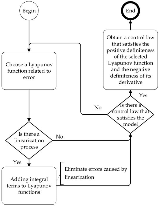
Figure 1.
Flowchart of Lyapunov function and control law.
Definition 1.
A family of mappings W is called a nonlinear semigroup in a normed space . If for every and some , the following conditions are satisfied:
- (i)
- , for all
- (ii)
- for all .
Definition 2.
A stationary point u is called
- (i)
- Stable (in sense of A.M. Lyapunov), if for any neighborhood of u there exists a neighborhood (i.e., not necessarily the same neighborhood) of the same point, such that for all (a certain value of u) ;
- (ii)
- Asymptotically stable (in sense of A.M. Lyapunov), if it is stable and for any point v in some neighborhood of u, for .
Theorem 1.
Let u be a stationary point. If there exists a Lyapunov function V such that
- (i)
- V(u) = 0
- (ii)
- . Here, φ is strictly increasing continuous function such that φ(0) = 0 and φ(r) > 0 for ; this indicates the point u is stable.
Theorem 2.
Let the conditions of Theorem 1 be satisfied and a strictly increasing continuous function ψ, such that ψ(0) = 0 and ψ(r) > 0 for exist. If , then the point u is asymptotically stable.
2.1. Design of the d-Axis Voltage Controller
A diagram of the SEIG–STATCOM system is shown in Figure 2, which consists of SEIG, STATCOM and static/dynamic loads. The parameter with the arrow pointing downwards is the measurement value required for control. An induction generator can generate electrical energy when the rotational speed of the rotor is greater than that of the synchronous speed of the induction motor and there is residual magnetism in the magnetic core of the induction motor. Then, the process self-excited voltage building is completed [30].
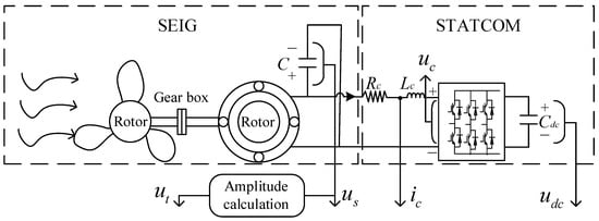
Figure 2.
Schematic diagram of SEIG–STATCOM.
STATCOM is utilized to compensate reactive power for voltage regulation. We assume that the no-load SEIG–STATCOM is in equilibrium. The dynamic model in dq-axis is described as follows [31]:
where Rc and Lc are the line resistance and inductance of the SEIG–STATCOM, respectively. Cdc is the capacitance of the DC side capacitor. Sd and Sq are the switching function on the dq-axis, respectively. ω is the synchronously rotating angle speed. udc is the DC side voltage. usd and usq are the dq-axis voltages of the point of common coupling (PCC), respectively. ucd and ucq are the AC side dq-axis output voltages of STATCOM, respectively. icd and icq are the dq-axis currents of STATCOM, respectively.
Neglecting the line losses and dead-time effects of the STATCOM, Equation (1) can be rearranged as follows:
We assume that the SEIG has already reached a stable operating state and that the line voltage has aligned with the d-axis direction. It has usd = ut* = 311 V and usq = 0 V. Moreover, uDC = udc2 and uDC* = (udc*)2. udc* is the reference DC voltage of the STATCOM. The error of the squared DC voltage is defined as eDC = uDC* − uDC. Its derivative is expressed as Equation (3).
Equation (2) is linearly processed, ignoring impedance. To ensure zero-error tracking, a Lyapunov function incorporating an integral term was selected based on Figure 1, as shown in Equation (4).
where VDC is semi-positive definite and K2>0. Taking the derivative of VDC yields the following:
when in Equation (5). Then, is semi-negative definite, the d-axis voltage loop controller achieves Lyapunov stability and the d-axis reference current is solved as follows:
where K1 > 0. can be regarded as the proportional parameter of the PI controller, while is equivalent to the integral parameter.
2.2. Design of the q-Axis Voltage Controller
Based on the instantaneous power theory, the PCC voltage drop is obtained as follows:
where ut and ut* present the amplitude voltage and its reference of PCC. P is the active power consumed in the transmission line, Q is the reactive power and U is the effective value of the line-to-line voltage. Xc is the inductive impedance. The relationship between icd and icq can be expressed as Equation (8):
where ut* = U = 311 V. The model in Equation (1) can be represented using the amplitude–phase relationship as follows:
Therefore, combining Equations (8) and (9), can be obtained as follows:
A Lyapunov function on q-axis is constructed as follows:
where K3 > 0 is a voltage controller parameter in q-axis and Vt is positive semidefinite. Thus, the derivative of the Lyapunov function (11) can be written as follows:
when , the q-axis reference current is evaluated as follows:
Then,
This indicates that the voltage loop controller of the q-axis is stable.
2.3. Design of the Current Controller
The dual-input dual-output (DIDO) system Equation (1) inherently complicates the endeavors of performance assessment and control synthesis. If f is a certain parameter, we define complex vectors as fdq = fd + jfq.
The complex vector of the current is a state variable. We set , and . In control law design, it is assumed that the current in non-coupled parts has already tracked the given value.
Define state variable error . To satisfy , the Lyapunov function V is defined as Equation (17).
A virtual control variable m is introduced to ensure that the selected Lyapunov function V is positive definite and its derivative is negative definite.
where m is a virtual coefficient greater than 0 to ensure Lyapunov global asymptotic stability. Replace Equation (20) with the component form of the d and q-axes to obtain the inner loop control law, as shown in Equation (22).
3. Results
3.1. Analysis of the Controller
The traditional control method and proposed method are shown in Figure 3a,b. “s” is a complex variable and can be regarded as a derivative operator in the complex frequency domain.
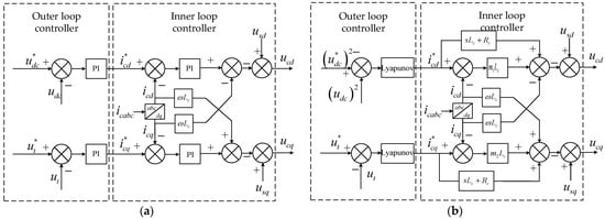
Figure 3.
Outer–inner loop of controller: (a) VOC (traditional control method); (b) LBC.
It can be inferred from the above design that m is a virtual coefficient greater than 0 to ensure the Lyapunov global asymptotic stability, whereas its upper bound remains undetermined. To estimate the effects of time delay and virtual coefficient on the current inner loop, a current inner loop controller and its controlled plant are illustrated in Figure 4. For the convenience of sensitivity analysis, we define the controller subscript n as the nominal value and the controlled plant as the actual value. The two blocks with the smallest time constants (sample, hold and the PWM) are grouped together to form a single block [25].
where TCD is the total delay which can be considered as a one order inertial link. Ts and TPWM denote the sampling delay and PWM delay, respectively. τCD presents the equivalent time constant of control loop.
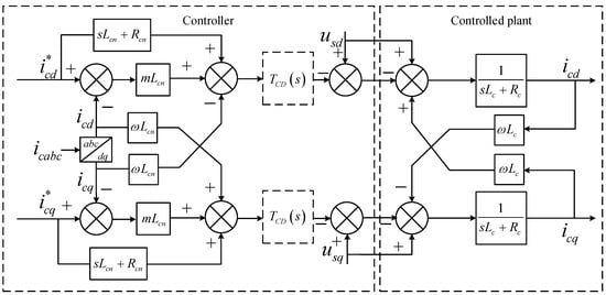
Figure 4.
Inner loop control block diagram.
The closed-loop transfer function without time delay is represented by the following matrix G. The feedforward term virtual coefficient is set as the same value and is denoted as mLc.
From a structural perspective, the decoupling can be seen as a feedback decoupling and the differential feedforward term replaces the difference integral term. It has and . When the nominal value approaches the actual value, we refer to it as fully tracking (). Due to the symmetry of the dq-axis transfer function, only the d-axis current transfer function is analyzed. Logarithmic sensitivity can be expressed as and . The Bode plot of logarithmic sensitivity is shown in Figure 5. From Figure 5, it can be seen that increasing m can reduce the sensitivity of the proposed method to impedance.
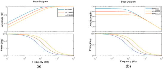
Figure 5.
The Bode plot of logarithmic sensitivity: (a) sensitivity to Lc; (b) sensitivity to Rc.
The closed-loop transfer function with time delay, and without considering the nominal values (Lcn = Lc, Rcn = Rc), is represented by the following matrix H.
According to Equation (14), the zero-pole plot of the current closed-loop system can be obtained. From Figure 6, the distribution of the pole point is confined to the left half-plane of the s-plane, implying that the selection of m will not affect the stability of the current loop. As m increases from 10,000 to 100,000 with a step size of 10,000, the zero will move away from the imaginary axis, indicating a faster response time of the current loop. However, the conjugate poles will move away from the real axis, leading to current loop overshoot and oscillations. In practical engineering applications, it is not desirable to have excessive current overshoot and oscillations, as this may lead to overcurrent conditions.
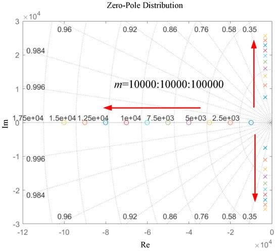
Figure 6.
The zero-pole distribution of the current closed-loop transfer function.
3.2. Simulation Results
In this section, the 2022b version of MATLAB/Simulink are executed to validate the efficiency of the proposed method; the mathematical model of the SEIG–STATCOM is built as Figure 7. The simulation parameters are shown in Table 1.
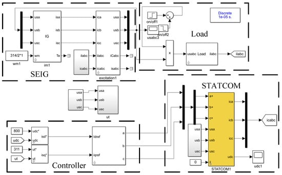
Figure 7.
The mathematical model of the SEIG–STATCOM in Simulink.

Table 1.
Main parameters of the simulation.
To ensure a fair comparison between the two methods, we present the performance of the traditional approach’s d-axis voltage loop under various parameter settings. The dynamic performance of the d-axis PI controller using various parameters is shown in Figure 8. Given the identical q-axis voltage loop structure between the proposed and the traditional approach, we employ the same parameters. Moreover, a zero-pole cancelation method is used in the inner loop parameters tuning. We choose the KvdP and KvdI as 0.3 and 3, respectively.
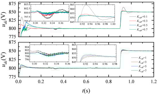
Figure 8.
The dynamic performance of the d-axis PI controller.
After the stable operation of SEIG self-excited voltage building, an IM load is applied at 0.3 s. This IM load was cut off at 0.6s and the DC voltage reference was changed at 0.9 s.
The proposed control strategy involves the separation of the controller into two loops: the inner loop and the outer loop, which are designed independently. We compare the performance of the control strategy using the following:
- PI (outer) + LBC (inner);
- LBC (outer) + PI (inner);
- The traditional approach VOC: PI (outer) + PI (inner).
Transient process indicators include voltage dip (this refers to the short-term rapid decrease in the effective value of the supply voltage to the rated value (90~10%)) and transient state (the time it takes for a system to transition from one transient state to another after being subjected to external disturbances or internal changes).
As depicted in Figure 9, the proposed method exhibits improved dynamic performance compared to the traditional approach. The LB (inner controller) reduces the DC side voltage drop by 0.2 V and the terminal voltage drop by 8.8 V, relative to the VOC. Similarly, the LB (outer controller) reduces the DC side voltage drop by 1.6 V and the terminal voltage drop by 6.8 V, also in comparison to the VOC. The LB (outer controller) will recover to its original value within approximately 0.5 ms. Compared with using LB (inner controller) and VOC, the DC transient time of using LB (outer controller) is reduced to about 1/4. It can be seen that using an outer loop LBC mainly improves the transient process of DC voltage, and using an inner loop LBC mainly improves the transient process of AC voltage.
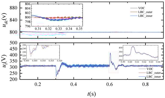
Figure 9.
The dynamic performance of the proposed and VOC.
3.3. Experiment Results
The system is based on the 2014b version of MATLAB/Simulink platform and provides a software and hardware working platform for controlling system development and semi-physical simulation. The feature of the dSPACE system is its seamless connection with MATLAB/Simulink, allowing for the direct generation of code from Simulink block diagrams and downloading to target hardware, achieving key functions such as rapid control prototyping (RCP) and hardware in the loop simulation (HILS).
In the power generation system, the prime mover is driven by a variable frequency drive to rotate at high speed, simulating the prime mover’s driving of the generator. When the variable frequency drive is set to 42 Hz, the self-excitation build-up process is completed. Due to the presence of residual magnetism within the generator, self-excitation oscillations can be achieved by connecting capacitors in parallel, ultimately realizing voltage stabilization through magnetic saturation. Three self-healing excitation capacitors of 47 μF, connected in delta form, and a power transistor adopt PM300DVA120, which has high integration, integrating IGBT (Insulated Gate Bipolar Transistor) and freewheeling diode. To ensure the safety of experimental equipment and personnel, we conducted experiments at the low voltage end of the transformer. The main circuit is shown in Figure 10b.
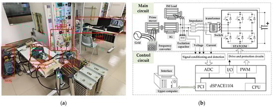
Figure 10.
Prototype experiment: (a) experimental platform of power generation system; (b) experiment block diagram of voltage regulation for SEIG.
The parameters of the IM and SEIG are consistent with the simulation, and parameters that have been changed are shown in Table 2. The experiment is carried out using the DS1104 control board for the various strategies. The SEIG–STATCOM setup is shown in Figure 10a.
Table 2.
Main parameters of the experiment.
When STATCOM is not connected to the SEIG, the performance of terminal voltage shown in Figure 11 after the IM load is applied. SEIG cannot restore its original terminal voltage and there is a voltage difference of 7.2 V.
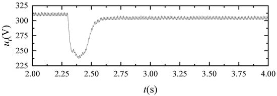
Figure 11.
The performance of terminal voltage without STATCOM.
At 1.83 s, an IM load is applied. Figure 12 shows the comparison of the dynamic responses of the STATCOM with the proposed LB (inner controller) and VOC. Compared to the VOC, the LB (inner controller) reduces the DC side voltage drop by 5.4 V and the terminal voltage drop by 4.6 V, respectively.
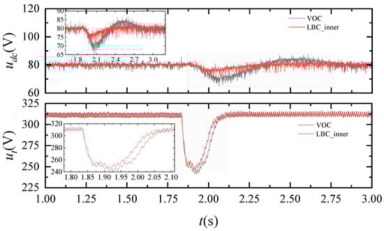
Figure 12.
The dynamic performance of the LBC (inner controller) and VOC.
Figure 13 shows the comparison of the dynamic responses of the STATCOM with the proposed LB (outer controller) and VOC. Compared to the VOC, the LB (outer controller) reduces the DC side voltage drop by 5.9 V. The structure of the outer loop q-axis LB is consistent with that of VOC, so the performance is similar, but there is randomness in the experiment and it cannot be completely consistent.
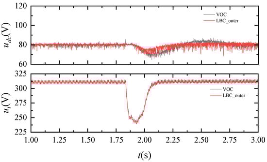
Figure 13.
The dynamic performance of the LBC (outer controller) and VOC.
Compared with Figure 10, connecting STATCOM enhances the voltage regulation capability of SEIG. We quantitatively evaluated the performance in the experiment and recorded it, as shown in Table 3.
Table 3.
Evaluation of SEIG’s voltage.
4. Conclusions
A novel LBC strategy for SEIG–STATCOM systems has been proposed in this paper. The dq-axis voltage loop and current loop were designed by selecting a proper Lyapunov function, separately. The research conclusions of this article are as follows:
- (1)
- The proposed LBC (outer loop on d-axis) achieves linearized voltage control with a quadratic outer loop structure; LBC (outer loop on q-axis) provides theoretical support for obtaining the q-axis reference current through proportional integration of the terminal voltage error.
- (2)
- A transfer function analysis was conducted on the inner loop of the proposed method, demonstrating its effectiveness in achieving decoupling and current tracking.
- (3)
- SEIG connected to STATCOM effectively improves voltage regulation capability and shortened the process of the transient by about 3.1 ms. Compared to traditional VOC, the outer loop LBC has an effect on shortening the transient processes of DC voltage by about 9.4 ms and the inner loop LBC has an effect on shortening the transient processes of both AC and DC voltages by about 2.6 ms and 8.7 ms, respectively. The simulation and experiment results show that the proposed LBC outperforms traditional methods.
However, there are some shortcomings in this article, such as the lack of analysis of the outer loop. The inner loop of the proposed method did not analyze the deviation of actual values from nominal values in sensitivity analysis. We will improve this part in future work.
Author Contributions
Conceptualization, Z.Z. and P.G.; Methodology, Z.Z.; Writing—review & editing, Z.Z.; Supervision, P.G.; Project administration, Z.L.; Funding acquisition, P.G. and Z.L. All authors have read and agreed to the published version of the manuscript.
Funding
This research was funded by The Natural Science Foundation of Guangxi Zhuang Autonomous Region, grant number 2018GXNSFDA138008, and The 2024 Middle-aged and Young Teachers’ Basic Ability Promotion Project of Guangxi, grant number 2024KY0011.
Data Availability Statement
The raw data supporting the conclusions of this article will be made available by the authors on request.
Conflicts of Interest
The authors declare no conflicts of interest.
Nomenclature
| Classification | Symbol | Quantity |
| Measured value | Rc | The actual line resistance of SEIG–STATCOM |
| Measured value | Lc | The actual line inductance of SEIG–STATCOM |
| Known value | Rcn | The nominal line resistance of SEIG–STATCOM |
| Known value | Lcn | The nominal line inductance of SEIG–STATCOM |
| Measured value | Cdc | The capacitance of DC side capacitor |
| Defined variable | Sd, Sq | The switching function on dq-axis |
| Known value | ω | The synchronously rotating angle speed |
| Measured value | udc | The voltage of DC side |
| Measured value | ut | The voltage amplitude of PCC |
| Measured value | usd, usq | The voltages of PCC on dq-axis |
| Known value | ucd, ucq | The output voltages of STATCOM on dq-axis |
| Measured value | icd, icq | The currents of STATCOM on dq-axis |
| Known value | (·)* | The reference value of a certain value |
| Measured value | uDC | uDC = (udc)2 |
| Defined variable | VDC | The Lyapunov function of the outer loop on d-axis |
| Defined variable | Vt | The Lyapunov function of the outer loop on q-axis |
| Defined variable | V | The Lyapunov function of the inner loop |
| Defined variable | edc | The error of DC voltage |
| Defined variable | eDC | The error of DC voltage’ square |
| Defined variable | et | The error of PCC voltage |
| Defined variable | e | The error of current |
| Measured value | Xc | The inductive reactance of SEIG–STATCOM |
| Measured value | U | The effective value of the line-to-line voltage |
| Measured value | P, Q | The active and reactive power consumed |
| Known value | τCD | The equivalent time constant of control loop |
| Control parameters | KvdP, KvqP | The voltage loop proportional gain on dq-axis |
| Control parameters | KvdI, KvqI | The voltage loop integral gain on dq-axis |
| Control parameters | KiP, KiI | The current loop proportional and integral gain |
| Control parameters | K1, K2 | The voltage loop virtual coefficient on d-axis |
| Control parameters | K3, K4 | The voltage loop virtual coefficient on q-axis |
| Control parameters | m1, m2 | The current loop virtual coefficient on dq-axis |
References
- Østergaard, P.A.; Duic, N.; Noorollahi, Y.; Kalogirou, S.A. Recent advances in renewable energy technology for the energy transition. Renew. Energy 2021, 179, 877–884. [Google Scholar] [CrossRef]
- Wei, Y.; Kang, L.; Huang, Z.; Li, Z. A magnetic energy recovery switch based terminal voltage regulator for the three-phase self-excited induction generators in renewable energy systems. J. Power Electron. 2015, 15, 1305–1317. [Google Scholar] [CrossRef][Green Version]
- Krishna, V.M.; Sandeep, V.; Murthy, S.; Yadlapati, K. Experimental investigation on performance comparison of self excited induction generator and permanent magnet synchronous generator for small scale renewable energy applications. Renew. Energy 2022, 195, 431–441. [Google Scholar] [CrossRef]
- Calgan, H.; Demirtas, M. A robust LQR-FOPIλDµ controller design for output voltage regulation of stand-alone self-excited induction generator. Electr. Power Syst. Res. 2021, 196, 107175. [Google Scholar] [CrossRef]
- Krishna, V.M.; Sandeep, V.; Narendra, B.; Prasad, K. Experimental study on self-excited induction generator for small-scale isolated rural electricity applications. Results Eng. 2023, 18, 101182. [Google Scholar] [CrossRef]
- Singh, B.; Murthy, S.S.; Chilipi, R.S.R. STATCOM-based controller for a three-phase SEIG feeding single-phase loads. IEEE Trans. Energy Convers. 2014, 29, 320–331. [Google Scholar]
- Wang, H.; Wu, X.; You, R.; Li, J. Modeling and analysis of SEIG-STATCOM systems based on the magnitude-phase dynamic method. J. Power Electron. 2018, 18, 944–953. [Google Scholar]
- Saidur, R. A review on electrical motors energy use and energy savings. Renew. Sustain. Energy Rev. 2010, 14, 877–898. [Google Scholar] [CrossRef]
- Prakash, S.B.; Sagar, M.P. Fuzzy Logic Controlled Based STATCOM to Compensate Loads for SEIG System. Int. J. Sci. Eng. Technol. Res. 2016, 5, 4048–4054. [Google Scholar]
- Xia, Y.; Peng, Y.; Yang, P.; Yu, M.; Wei, W. Distributed coordination control for multiple bidirectional power converters in a hybrid AC/DC microgrid. IEEE Trans. Power Electron. 2016, 32, 4949–4959. [Google Scholar] [CrossRef]
- Dyanamina, G.; Kakodia, S.K. SEIG voltage regulation with STATCOM Regulator using Fuzzy logic controller. In Proceedings of the 2021 International Conference on Sustainable Energy and Future Electric Transportation (SEFET), Hyderabad, India, 21–23 January 2021; pp. 1–6. [Google Scholar]
- Ansari, J.; Abbasi, A.R.; Heydari, M.H.; Avazzadeh, Z. Simultaneous design of fuzzy PSS and fuzzy STATCOM controllers for power system stability enhancement. Alex. Eng. J. 2022, 61, 2841–2850. [Google Scholar] [CrossRef]
- Das, M.; Giribabu, D. ANFIS controller based STATCOM regulator for self excited induction generator. In Proceedings of the 2016 IEEE 6th International Conference on Power Systems (ICPS), New Delhi, India, 4–6 March 2016; pp. 1–6. [Google Scholar]
- Singh, P.D.; Gao, S. Clean and sustainable micro hydro power generation using parallel variable asynchronous generators controlled by AC-DC-AC converter and fuzzy PSO/PI D-STATCOM for remote areas. Sustain. Cities Soc. 2022, 77, 103527. [Google Scholar] [CrossRef]
- Mokhtari, M.; Zouggar, S.; M’sirdi, N.K.; Elhafyani, M. Sliding Mode & Single Input Fuzzy Logic Controllers for Voltage Regulation Of an Asynchronous Wind Turbine Using STATCOM. IFAC-PapersOnLine 2020, 53, 12803–12808. [Google Scholar]
- Oliveira, T.R.; Hsu, L.; Nunes, E.V.L. Smooth sliding control to overcome chattering arising in classical SMC and super-twisting algorithm in the presence of unmodeled dynamics. J. Frankl. Inst. 2022, 359, 1235–1256. [Google Scholar] [CrossRef]
- Furat, M. Chattering attenuation analysis in variable structure control for automatic voltage regulator with input constraints. Eng. Sci. Technol. Int. J. 2023, 45, 101499. [Google Scholar] [CrossRef]
- Ullah, M.F.; Hanif, A. Power quality improvement in distribution system using distribution static compensator with super twisting sliding mode control. Int. Trans. Electr. Energy Syst. 2021, 31, e12997. [Google Scholar] [CrossRef]
- Sefa, I.; Ozdemir, S.; Komurcugil, H.; Altin, N. An enhanced Lyapunov-function based control scheme for three-phase grid-tied VSI with LCL filter. IEEE Trans. Sustain. Energy 2018, 10, 504–513. [Google Scholar] [CrossRef]
- Rahmani, S.; Hamadi, A.; Al-Haddad, K. A Lyapunov-function-based control for a three-phase shunt hybrid active filter. IEEE Trans. Ind. Electron. 2011, 59, 1418–1429. [Google Scholar] [CrossRef]
- Dasgupta, S.; Mohan, S.N.; Sahoo, S.K.; Panda, S.K. Lyapunov function-based current controller to control active and reactive power flow from a renewable energy source to a generalized three-phase microgrid system. IEEE Trans. Ind. Electron. 2012, 60, 799–813. [Google Scholar] [CrossRef]
- Bayhan, S.; Seyedalipour, S.S.; Komurcugil, H.; Abu-Rub, H. Lyapunov energy function based control method for three-phase UPS inverters with output voltage feedback loops. IEEE Access 2019, 7, 113699–113711. [Google Scholar] [CrossRef]
- Beheshti, N.; Rezanejad, M.; Mehrasa, M. Linearized control technique with Lyapunov function-based compensators for MMC-based HVDC system under load variation and fault condition. Int. J. Electr. Power Energy Syst. 2021, 124, 106333. [Google Scholar] [CrossRef]
- He, J.; Zhang, X.; Ma, H.; Cai, C. Lyapunov-based large-signal control of three-phase stand-alone inverters with inherent dual control loops and load disturbance adaptivity. IEEE Trans. Ind. Electron. 2020, 68, 8391–8401. [Google Scholar] [CrossRef]
- Blasko, V.; Kaura, V. A new mathematical model and control of a three-phase AC-DC voltage source converter. IEEE Trans. Power Electron. 1997, 12, 116–123. [Google Scholar] [CrossRef]
- Harnefors, L.; Wang, X.; Chou, S.-F.; Bongiorno, M.; Hinkkanen, M.; Routimo, M. Asymmetric complex-vector models with application to VSC–grid interaction. IEEE J. Emerg. Sel. Top. Power Electron. 2020, 8, 1911–1921. [Google Scholar] [CrossRef]
- Wu, L.; Li, J.; Lu, Y.; Yang, K.; He, K.; Chen, H.; Chen, Z. Design of complex vector controller for high-power induction machine drive. IEEE Trans. Transp. Electrif. 2023, 10, 1816–1826. [Google Scholar] [CrossRef]
- Xiao, Q.; Tang, F.; Xin, Z.; Zhou, J.; Chen, P.; Loh, P.C. Large time-delay decoupling and correction in synchronous complex-vector frame. IET Power Electron. 2019, 12, 254–266. [Google Scholar] [CrossRef]
- Moskvicheva, P.O.; Semenova, I.N. The Lyapunov stability of the Cauchy-Dirichlet problem for the generalized Hoff equation. Весmнuк Южнo-Уpaльcкoгo Гocyдapcmвeннoгo Унuвepcumema. Cepuя Mameмamuчecкoe Moдeлupoвaнue И Пpoгpaммupoвaнue 2014, 7, 126–131. [Google Scholar] [CrossRef]
- Varshney, L.; Vardhan, A.S.S.; Vardhan, A.S.S.; Kumar, S.; Saket, R.; Sanjeevikumar, P. Performance characteristics and reliability assessment of self-excited induction generator for wind power generation. IET Renew. Power Gener. 2021, 15, 1927–1942. [Google Scholar] [CrossRef]
- Xu, Y.; Li, F. Adaptive PI control of STATCOM for voltage regulation. IEEE Trans. Power Deliv. 2014, 29, 1002–1011. [Google Scholar] [CrossRef]


Disclaimer/Publisher’s Note: The statements, opinions and data contained in all publications are solely those of the individual author(s) and contributor(s) and not of MDPI and/or the editor(s). MDPI and/or the editor(s) disclaim responsibility for any injury to people or property resulting from any ideas, methods, instructions or products referred to in the content. |
© 2024 by the authors. Licensee MDPI, Basel, Switzerland. This article is an open access article distributed under the terms and conditions of the Creative Commons Attribution (CC BY) license (https://creativecommons.org/licenses/by/4.0/).