
Heating Energy Performance Gap in Vulnerable Households: Identification and Impact of Associated Variables


 , and
, and
Abstract
:1. Introduction
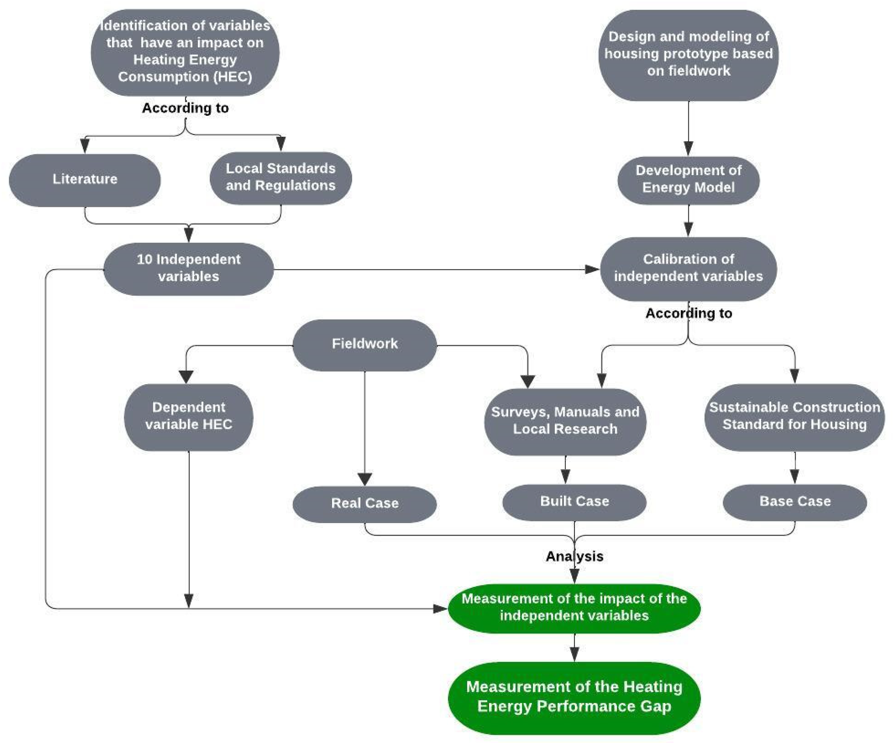
2. Methodology
2.1. Identification of Relevant Parameters
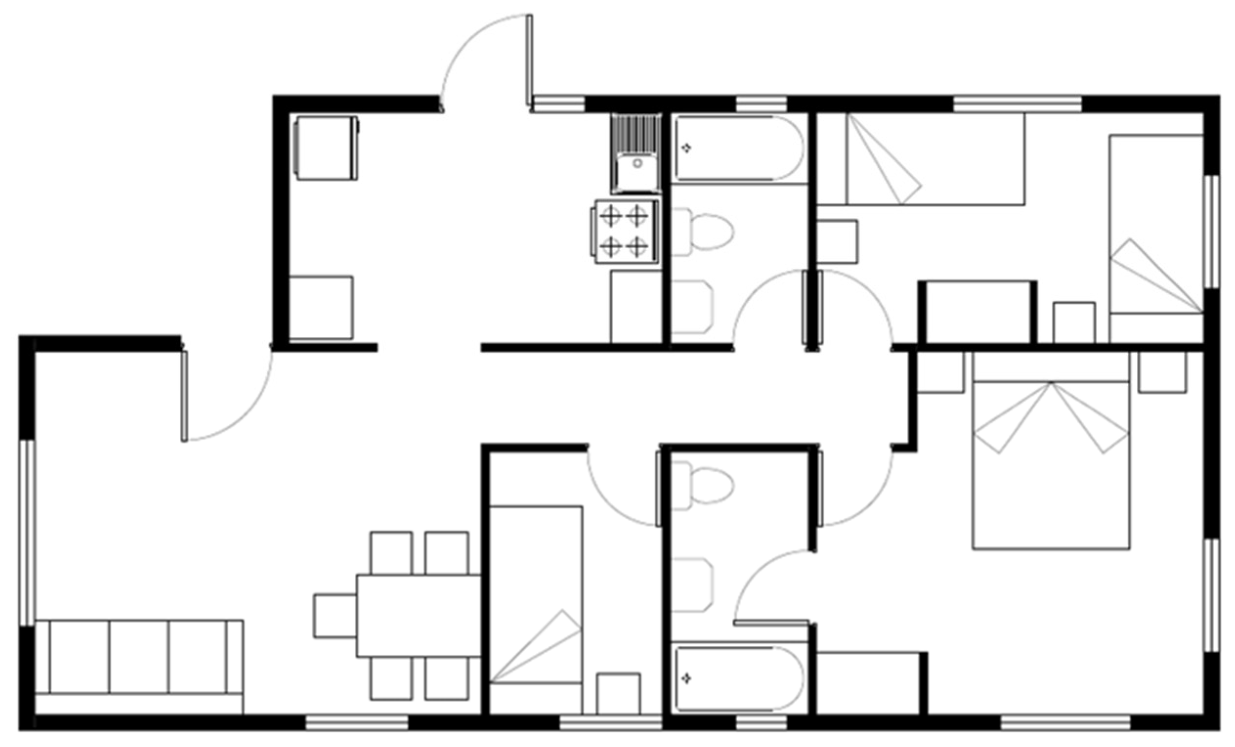
2.2. Selection and Characterization of the Case Study
2.2.1. Determination of the Case Study
2.2.2. Sample
2.2.3. Survey
2.3. Definition of Values for Variables
2.4. Real Case
Base Case Modeling
3. Results
3.1. Characterization of Variables

| Variable | Base Case | Built Case | |
|---|---|---|---|
| V01 | Infiltrations | The maximum air infiltration class allowed for the thermal envelope of buildings in the Biobío region is 8.00 ac/h at 50 Pa. | The surveys conducted in the study showed half-timbered houses as the most representative case, whose representative value is 24.6 ac/h at 50 Pa [41]. |
| V02 | Climate file | Climate file with Energy Plus Weather format (epw), available for free on the csustentable.minvu.gob.cl website. There were only 20 files for the whole country on the platform, so the one closest to the study area is used, which is Concepcion-Estaciones.epw. | The data from the 2020 Human Weather Station were used. This is the climate source closest to the commune of Mulchén, which is 25 km from the city center. |
| V03 | Ground Temperature | This variable is not considered in the Standard. | This variable was included because it contributed to the simulations and, according to the study of [34], approximated the realities of the environment. Although these values could not be provided in the field, the ground temperature was validated in the model with the Ground Domain (GD) tool in DB and is associated with the temperature of the previous variable. This considers the gravel-based ground characteristic of the area, with a conductivity of 0.5 W/m K, a heat capacity of 184.0 J/kg-K, a density of 2050.0 kg/m3, a ground domain depth of 10 m, and an incidence perimeter of 5 m. |
| V04 | Air-conditioning setpoints | 90% acceptability of the ASHRAE 55 adaptive thermal comfort model [42], calibrated with monthly temperatures. | 80% acceptability of the ASHRAE 55 adaptive thermal comfort model [42], calibrated with daily temperatures. |
| V05 | COP | ECSV does not include wood-fired equipment specifying that the performance must be greater than or equal to 100%. | The performance coefficient of the typical heaters used by the studied households was adopted following questions Q91 and Q93, a double-chambered wood-burner, supported by the study of [39], with an efficiency of 70%, according to the Bosca Wood-burning Heaters User Manual. |
| V06 | Lighting load | 1.5 W/m2. | The data for this variable were obtained thanks to the questions asked in Appendix A, where the average of question Q119 was measured, resulting in a power of 3.7 W/m2. |
| V07 | Lighting usage schedule | January–February/November–December 21–22 h. March–April/September–October 7–8 h/20–22 h. May–August 7–8 h/18–22 h. | The lighting activation schedule stated by the inhabitants of the surveyed dwellings established two and a half hours of use 365 days a year, according to the average from question Q120 in Appendix A. |
| V08 | Number of people | They will be used with an occupation following NCh 3308:2013, which determines a minimum of two people, plus one for each bedroom. | According to the surveys, the average number of inhabitants per dwelling is three people, as per question Q14 in Appendix A. |
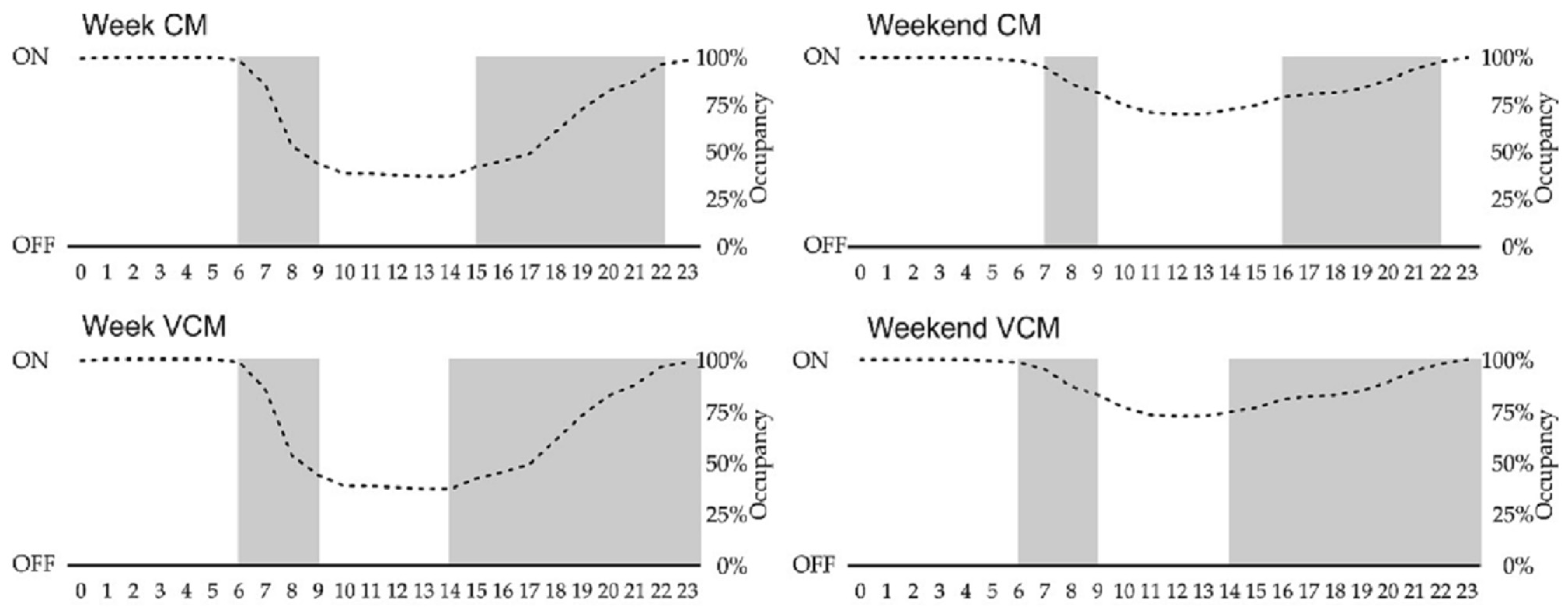
| V09 | Air-conditioning schedule | The thermal demand is calculated to permanently reach the comfort levels 24/7, regardless of the house’s actual use schedule. | The schedule profile is summarized in the number of hours stated in the surveys and the exact time of turning on during the day according to the study’s Week CM profile (weekday in a cold month) [37], with the period detailed in Table 6. |
| V10 | Natural Ventilation | Between 10 p.m. and 6 a.m. and when the outside temperature exceeds 15 °C (8 h). | Two hours a day are stated, following the mode arising from questions Q50–52. |
| Schedule from–to | ||||
|---|---|---|---|---|
| March–April | May–August | September | October | |
| GMT-3 | GMT-4 | GMT-3 | GMT-3 | |
| Surveys | 6–9/17–23 h | 6–9/17–24 h | 6–9/17–23 h | 6–9/17–24 h |
3.2. Simulation of Variables
3.2.1. Dependent Variable, Heating Energy Consumption
3.2.2. Independent Variables
3.3. Measuring the Impact of Variables and the Heating Energy Performance Gap
4. Discussion
5. Conclusions
Author Contributions
Funding
Data Availability Statement
Acknowledgments
Conflicts of Interest
Appendix A
| Section | Code | Question | Type of Response | Variable |
| Section 3: Household information | Q14 | How many people are in your family group? Please select one option for each row. If there are no people in a certain age range, select 0. | Infants (1 to 5 years)/(0/1/2/3/4 or more members) Children (6 to 12 years old)/(0/1/2/3/4 or more members) Teenagers (12 to 20 years old)/(0/1/2/3/4 or more members) Adults (21 to 59 years)/(0/1/2/3/4 or more members) Seniors (60 years or more)/(0/1/2/3/4 or more members) | Number of people |
| Section 4: Characteristics of the dwelling | Q25 | Is your home detached, semi-detached, or terraced? | Architectural Typology | |
| Q26 | How many floors does your home have? | Short answer | Architectural Typology | |
| Q27 | What surface area (approximate square meters) does your home have? Write only the number, and do not consider the patio, garden, or terrace | Architectural Typology | ||
| Q30 | How many bedrooms does your dwelling have? | (1, 2, 3, 4, 5, 6, more than 6) | Architectural Typology | |
| Q31 | What is the primary material of your home’s wall structure? | (Concrete; Brick; Concrete Block; Wood; Adobe; SIP Panels; Metalcon; Other; I don’t know) | U-value | |
| Q32 | What is the primary structural material of the walls of the first floor of your home? | (Concrete; Brick; Concrete Block; Wood; Adobe; SIP Panels; Metalcon; Other; I don’t know) | U-value | |
| Q33 | What is the primary structural material of the walls of the second floor of your home? | (Concrete; Brick; Concrete Block; Wood; Adobe; SIP Panels; Metalcon; Other; I don’t know) | U-value | |
| Q34 | What is the primary structural material of your home’s roof? | (Tiles (clay, metal, cement, wood, asphalt); Concrete slab; Metal plates (zinc, copper, etc.); Fiber cement plates (slate); Phonolite or tarred felt sheets; Straw, thatch, bullrush, or cane; Other). | U-value | |
| Q35 | What is the primary material of your home’s floor? | (Parquet, wood, laminated flooring, or similar; Porcelain, flexit, or similar tiles; Carpet or floor covering; Cement tile; Concrete slab; Earth) | U-value | |
| Q36 | Does your home have thermal insulation in the following elements (wall, ceiling, floor)? Refers to the insulating material inside walls, ceilings, or floors, commonly known as expanded polystyrene (Styrofoam), mineral wool, or others. | Yes/No/I don’t know | U-value | |
| Section 5: Features of the dwelling’s windows | Q40 | What kind of glass do the windows of your home have? | Single glazing, double glazing, I don’t know | U-value |
| Q45 | What kind of materiality do the frames of your windows have? | Aluminum steel, PVC, wood, I don’t know | U-value | |
| Q50 | How often do you or someone else open the windows or doors to ventilate in summer? | Drop-down menu: More than once a day Every day or almost every day Not every day, but at least once a week Rarely or never | Natural ventilation schedule | |
| Q51 | How often do you or someone else open the windows or doors to ventilate in winter? | Drop-down menu: More than once a day Every day or almost every day Not every day, but at least once a week Rarely or never | Natural ventilation schedule | |
| Q52 | How long do you usually leave the windows or doors open to ventilate in summer? | Drop-down menu: Less than 5 min a day Between 5 to 15 min a day/Between 15 to 30 min a day/Between 30 min and 1 h a day/Between 1 to 2 h a day/Between 2 to 4 h a day/Most of the day (+4 h)/Rarely or I never close it completely, not even at night | Natural ventilation schedule | |
| Section 6: Energy | Q59 | On average, how much do you spend monthly on firewood during the SUMMER months? | I don’t pay for the service Less than CLP10,000/CLP11,000–20,000/CLP21,000-30,000/CLP31,000–40,000/CLP41,000–50,000/CLP51,000–60,000/CLP61,000–70,000/CLP71,000–80,000/CLP81,000–90,000/CLP91,000–100,000/More than CLP100,000 | Real Consumption |
| Q67 | On average, how much do you spend monthly on firewood during the WINTER months? | I don’t pay for the service Less than CLP10,000/CLP11,000–20,000/CLP21,000–30,000/CLP31,000–40,000/CLP41,000–50,000/CLP51,000–60,000/CLP61,000–70,000/CLP71,000–80,000/CLP81,000–90,000/CLP91,000–100,000/More than CLP100,000 | Real Consumption | |
| Section 9: Heating and cooling | Q89 | Which of the following systems do you mainly use to heat your home? | I do not have heating Fireplace, stove, heater, or some other appliance Central heating (radiators) or air-conditioning Fireplace, stove, heater, or some other appliance Central heating (radiators) or air-conditioning | Real Consumption |
| Q92 | What fuels or energy sources does the heater use in your home? Choose as many options as you want. | Piped gas, gas in cylinders, firewood, kerosene, pellets, other | Real Consumption | |
| Q93 | Is the heater a forced draft one? | Yes, No, I don’t know | Performance coefficient | |
| Q97 | During which months do you use the appliance to heat your home? | Drop-down menu with all the months of the year | Heating Schedule | |
| Q98 | During those months, on average, how long a day do you usually use the appliance for heating? | All the time (day and night) All day long 3–6 h a day 1–3 h a day Less than 1 h a day | Heating Schedule | |
| Section 10: Indoor temperature and comfort | Q105 | Which of the following systems do you mainly use to cool your home? | None, fan or other appliance, air-conditioning. | Cooling Schedule |
| Q107 | Which months do you use the fan or appliance to cool your home? | Drop-down menu with all the months of the year | Cooling Schedule | |
| Q108 | On average, how long a day do you usually use the fan or appliance to cool the house during those months? | All the time (day and night) All day long 3–6 h a day 1–3 h a day Less than 1 h a day | Cooling Schedule | |
| Section 11: Lighting | Q119 | What kind of bulb do you use in most rooms? | Incandescent, Halogen, Fluorescent, LED | Internal lighting load |
| Q120 | Approximately how many hours a day do the lights stay on in the following rooms? Bedroom, living room, dining room, kitchen, bathroom | Options: No lights, less than 2 h a day, between 2 and 5 h a day, more than 5 h a day | Lighting occupancy schedule |
References
- Geraldi, M.S.; Ghisi, E. Building-level and stock-level in contrast: A literature review of the energy performance of buildings during the operational stage. Energy Build. 2020, 211, 109810. [Google Scholar] [CrossRef]
- Zhang, Y.; Bai, X.; Mills, F.P.; Pezzey, J.C. Rethinking the role of occupant behavior in building energy performance: A review. Energy Build. 2018, 172, 279–294. [Google Scholar] [CrossRef]
- Pérez-Fargallo, A.; Bienvenido-Huertas, D.; Rubio-Bellido, C.; Trebilcock, M. Energy poverty risk mapping methodology considering the user’s thermal adaptability: The case of Chile. Energy Sustain. Dev. 2020, 58, 63–77. [Google Scholar] [CrossRef]
- Pérez-Fargallo, A.; Rubio-Bellido, C.; Pulido-Arcas, J.A.; Gallego-Maya, I.; Guevara-García, F.J. Influence of adaptive comfort models on energy improvement for housing in cold areas. Sustainability 2018, 10, 859. [Google Scholar] [CrossRef]
- Arbulu, M.; Perez-Bezos, S.; Figueroa-Lopez, A.; Oregi, X. Opportunities and Barriers of Calibrating Residential Building Performance Simulation Models Using Monitored and Survey-Based Occupant Behavioural Data: A Case Study in Northern Spain. Buildings 2024, 14, 1911. [Google Scholar] [CrossRef]
- Jain, N.; Burman, E.; Stamp, S.; Mumovic, D.; Davies, M. Cross-sectoral assessment of the performance gap using calibrated building energy performance simulation. Energy Build. 2020, 224, 110271. [Google Scholar] [CrossRef]
- Kampelis, N.; Gobakis, K.; Vagias, V.; Kolokotsa, D.; Standardi, L.; Isidori, D.; Cristalli, C.; Montagnino, F.; Paredes, F.; Muratore, P.; et al. Evaluation of the performance gap in industrial, residential & tertiary near-Zero energy buildings. Energy Build. 2017, 148, 58–73. [Google Scholar] [CrossRef]
- Mahdavi, A.; Berger, C.; Amin, H.; Ampatzi, E.; Andersen, R.K.; Azar, E.; Barthelmes, V.M.; Favero, M.; Hahn, J.; Khovalyg, D.; et al. The role of occupants in buildings’ energy performance gap: Myth or reality? Sustainability 2021, 13, 3146. [Google Scholar] [CrossRef]
- de Wilde, P. The gap between predicted and measured energy performance of buildings: A framework for investigation. Autom. Constr. 2014, 41, 40–49. [Google Scholar] [CrossRef]
- Attia, S.; Hamdy, M.; O’brien, W.; Carlucci, S. Assessing gaps and needs for integrating building performance optimization tools in net zero energy buildings design. Energy Build. 2013, 60, 110–124. [Google Scholar] [CrossRef]
- Zavrl, M.; Stegnar, G. Comparison of Simulated and Monitored Energy Performance Indicators on NZEB Case Study Eco Silver House. Procedia Environ. Sci. 2017, 38, 52–59. [Google Scholar] [CrossRef]
- Herrando, M.; Cambra, D.; Navarro, M.; de la Cruz, L.; Millán, G.; Zabalza, I. Energy Performance Certification of Faculty Buildings in Spain: The gap between estimated and real energy consumption. Energy Convers. Manag. 2016, 125, 141–153. [Google Scholar] [CrossRef]
- National Measurement Network. The Building Performance Gap-Closing It through Better Measurement Event Report; National Physical Laboratory: London, UK, 2012. [Google Scholar]
- Yan, D.; O’brien, W.; Hong, T.; Feng, X.; Gunay, H.B.; Tahmasebi, F.; Mahdavi, A. Occupant behavior modeling for building performance simulation: Current state and future challenges. Energy Build. 2015, 107, 264–278. [Google Scholar] [CrossRef]
- Menezes, A.C.; Cripps, A.; Bouchlaghem, D.; Buswell, R. Predicted vs. actual energy performance of non-domestic buildings: Using post-occupancy evaluation data to reduce the performance gap. Appl. Energy 2012, 97, 355–364. [Google Scholar] [CrossRef]
- André, P.; Georges, B.; Lebrun, J.; Lemort, V.; Teodorese, I.V. From model validation to production of reference simulations: How to increase reliability and applicability of building and HVAC simulation models. Build. Serv. Eng. Res. Technol. 2008, 29, 61–72. [Google Scholar] [CrossRef]
- van den Brom, P.; Meijer, A.; Visscher, H. Performance gaps in energy consumption: Household groups and building characteristics. Build. Res. Inf. 2018, 46, 54–70. [Google Scholar] [CrossRef]
- Szulgowska-Zgrzywa, M.; Stefanowicz, E.; Chmielewska, A.; Piechurski, K. Detailed Analysis of the Causes of the Energy Performance Gap Using the Example of Apartments in Historical Buildings in Wroclaw (Poland). Energies 2023, 16, 1814. [Google Scholar] [CrossRef]
- DellaValle, N.; Bisello, A.; Balest, J. In search of behavioural and social levers for effective social housing retrofit programs. Energy Build. 2018, 172, 517–524. [Google Scholar] [CrossRef]
- Szulgowska-Zgrzywa, M.; Stefanowicz, E.; Piechurski, K.; Chmielewska, A.; Kowalczyk, M. Impact of users’ behavior and real weather conditions on the energy consumption of tenement houses in wroclaw, poland: Energy performance gap simulation based on a model calibrated by field measurements. Energies 2020, 13, 6707. [Google Scholar] [CrossRef]
- Cozza, S.; Chambers, J.; Brambilla, A.; Patel, M.K. In search of optimal consumption: A review of causes and solutions to the Energy Performance Gap in residential buildings. Energy Build. 2021, 249, 111253. [Google Scholar] [CrossRef]
- Charlier, D. Explaining the energy performance gap in buildings with a latent profile analysis. Energy Policy 2021, 156, 112480. [Google Scholar] [CrossRef]
- Hu, S.; Yan, D.; Azar, E.; Guo, F. A systematic review of occupant behavior in building energy policy. Build. Environ. 2020, 175, 106807. [Google Scholar] [CrossRef]
- Bustamante, W.; Rozas, Y.; Cepeda, R.; Encinas, F.; Martínez, P. Guía de Diseño para la Eficiencia Energética en la Vivienda Social. Monogr. Ens. 2009, 333. [Google Scholar] [CrossRef]
- Molina, P. Normativa de Aislación Térmica y Calidad de Vida|Preservar. Available online: https://www.preservar.cl/normativa-de-aislacion-termica-gran-aliada-para-mejorar-la-calidad-de-vida-de-las-personas/ (accessed on 13 February 2023).
- Reyes, R.; Schueftan, A.; Ruiz, C.; González, A.D. Controlling air pollution in a context of high energy poverty levels in southern Chile: Clean air but colder houses? Energy Policy 2019, 124, 301–311. [Google Scholar] [CrossRef]
- Ministerio de Vivienda y Urbanismo—Minvu. Estándares de Construcción Sustentable Para Viviendas de Chile, Tomo ii Energía; Ministerio de Vivienda y Urbanismo: Santiago, Chile, 2018.
- Hernandez-Cruz, P.; Giraldo-Soto, C.; Escudero-Revilla, C.; Hidalgo-Betanzos, J.M.; Flores-Abascal, I. Energy efficiency and energy performance gap in centralized social housing buildings of the Basque Country. Energy Build. 2023, 298, 113534. [Google Scholar] [CrossRef]
- Pérez-Fargallo, A.; Marín-Restrepo, L.; Contreras-Espinoza, S.; Bienvenido-Huertas, D. Do we need complex and multidimensional indicators to assess energy poverty? The case of the Chilean indicator. Energy Build. 2023, 295, 113314. [Google Scholar] [CrossRef]
- Bustamante, W.; Encinas, F. Parámetros de Diseño y Desempeño Energético en Edificios de Clima Mediterráneo. ARQ 2012, 82, 116–119. [Google Scholar] [CrossRef]
- Martínez, P.W.; Kelly, M.T. Integración de criterios de desempeños en el mejoramiento energético-ambiental de viviendas sociales existentes en Chile. Ambiente Construído 2015, 15, 47–63. [Google Scholar] [CrossRef]
- Pérez-Fargallo, A.; Rubio-Bellido, C.; Pulido-Arcas, J.A.; Trebilcock, M. Development policy in social housing allocation: Fuel poverty potential risk index. Indoor Built Environ. 2017, 26, 980–998. [Google Scholar] [CrossRef]
- Pérez-Fargallo, A.; Pulido-Arcas, J.; Rubio-Bellido, C.; Trebilcock, M.; Piderit, B.; Attia, S. Development of a new adaptive comfort model for low income housing in the central-south of chile. Energy Build. 2018, 178, 94–106. [Google Scholar] [CrossRef]
- Azar, E.; O’Brien, W.; Carlucci, S.; Hong, T.; Sonta, A.; Kim, J.; Andargie, M.S.; Abuimara, T.; El Asmar, M.; Jain, R.K.; et al. Simulation-aided occupant-centric building design: A critical review of tools, methods, and applications. Energy Build. 2020, 224, 110292. [Google Scholar] [CrossRef]
- Pereira-Ruchansky, L.; Pérez-Fargallo, A. Integrated analysis of energy saving and thermal comfort of retrofits in social housing under climate change influence in uruguay. Sustainability 2020, 12, 4636. [Google Scholar] [CrossRef]
- Edalatnia, S.; Das, R.R. Building benchmarking and energy performance: Analysis of social and affordable housing in British Columbia, Canada. Energy Build. 2024, 313, 114259. [Google Scholar] [CrossRef]
- Ministerio de Desarrollo Social y Familia. Informe Final Panel de Expertos Para Mejoras al Instrumento de Focalización del Registro Social de Hogares; Ministerio de Vivienda y Urbanismo: Santiago, Chile, 2022.
- Ministerio del Medio Ambiente. Reporte de Leña Región de la Araucanía—MMA. Available online: https://mma.gob.cl/araucania/reporte-de-lena-region-de-la-araucania/ (accessed on 28 February 2023).
- CDT. Medición del Consumo Nacional de Leña y Otros Combustibles Sólidos Derivados de la Madera; Corporación de Desarrollo Tecnológico (CDT): Santiago, Chile, 2015. [Google Scholar]
- Ministerio de Energía. Calculadora de Biomasa—Autogeneración. Available online: https://autoconsumo.minenergia.cl/?p=2011 (accessed on 28 February 2023).
- Kelly, M.T. Manual de Hermeticidad al Aire de Edificaciones; Universidad del Bío-Bío: Concepción, Chile, 2014. [Google Scholar]
- de Dear, R.; Brager, G.S. Developing an adaptive model of thermal comfort and preference. ASHRAE Trans. 1998, 104, 1–19. [Google Scholar]
- Muñoz-Fierro, J.; Bobadilla-Moreno, A.; Bienvenido-Huertas, D.; Pulido-Arcas, J.A.; Pérez-Fargallo, A. Estimation of heating system energy modeling profiles based on environmental monitoring records in Central-Southern Chile. Energy Build. 2023, 292, 113153. [Google Scholar] [CrossRef]
- CDT. Informe Final de usos de la Energía de los Hogares Chile 2018; Corporación de Desarrollo Tecnológico/In Data: Santiago, Chile, 2019. [Google Scholar]
- Figueroa, R.; Martín, S.; Bobadilla, A.; Besser, D.; Días, M.; Arriagada, R.; Espinoza, R. Air infiltration in Chilean housing: A baseline determination. In Proceedings of the PLEA2013—29th Conference, Sustainable Architecture for a Renewable Future, Munich, Germany, 10–12 September 2013. [Google Scholar]
- Sonderegger, R.C. Movers and Stayers: The Resident’s Contribution to Variation across Houses in Energy Consumption for Space Heating*. Energy Build. 1978, 1, 313–324. [Google Scholar] [CrossRef]
- Kragh, J.; Rose, J.; Knudsen, H.N.; Jensen, O.M. Possible explanations for the gap between calculated and measured energy consumption of new houses. Energy Procedia 2017, 132, 69–74. [Google Scholar] [CrossRef]
- Sunikka-Blank, M.; Galvin, R. Introducing the prebound effect: The gap between performance and actual energy consumption. Build. Res. Inf. 2012, 40, 260–273. [Google Scholar] [CrossRef]
| Variables | ||||||||
|---|---|---|---|---|---|---|---|---|
| Source | Country | Köppen–Geiger Climate Classification | Climate | Envelope | Systems and Equipment | Operation and Maintenance | User Behavior | Indoor Environmental Quality |
| [24] | Chile | - | ● | ● | ● | ● | ● | ● |
| [32] | Chile | - | ● | ● | ● | ● | ● | |
| [17] | Netherlands | Cfb | ● | ● | ● | ● | ||
| [33] | Chile | Csb | ● | ● | ● | |||
| [34] | - | - | ● | ● | ● | ● | ● | ● |
| [1] | - | - | ● | ● | ● | ● | ● | ● |
| [6] | United Kingdom | Cfb | ● | ● | ● | ● | ||
| [23] | - | - | ● | ● | ● | ● | ● | ● |
| [35] | Uruguay | Cfa | ● | ● | ● | ● | ||
| [28] | Spain | Cfb | ● | ● | ● | ● | ● | ● |
| [36] | Canada | Dfc | ● | ● | ● | |||
| [20] | Poland | Cfb | ● | ● | ● | ● | ● | ● |
| Category | Variable | Unit |
|---|---|---|
| Envelope | Thermal transmittance of Walls | W/m2-K |
| Thermal transmittance of Roof | W/m2-K | |
| Thermal transmittance of Floor/Slab | W/m2-K | |
| Thermal transmittance of Glazing | W/m2-K | |
| Thermal transmittance of Doors | W/m2-K | |
| Infiltrations | ac/h at 50 Pa | |
| Climate | Climate File | - |
| Ground Temperature | °C | |
| Indoor environmental quality | Heating and Cooling Limit | °C |
| Natural Ventilation | ACH | |
| Systems and equipment | Performance coefficient | COP |
| Internal lighting load | W/m2 | |
| Occupant behavior | Lighting occupancy schedule | Hours per day |
| Number of people | People | |
| Heating act. hours | Hours per year | |
| Cooling act. hours | Hours per year | |
| Natural ventilation schedule | Hours per day | |
| Metabolic Index | W/person | |
| Internal loads schedule | Hours per day |
| Element | Int/Ext Layers | Thickness | Unit | U-Value | Unit |
|---|---|---|---|---|---|
| Walls | Plasterboard cardboard | 10.0 | mm | 3.4 | W/m2-K |
| OSB board | 9.5 | mm | |||
| Wooden decking | 2.5 | mm | |||
| Roof | Plasterboard cardboard | 10.0 | mm | 4.1 | W/m2-K |
| OSB board | 9.5 | mm | |||
| Floor/Slab | Wooden floor | 2.5 | mm | 1.5 | W/m2-K |
| Concrete base | 80.0 | mm | |||
| Sand | 100.0 | mm | |||
| Glazing | Generic single glazing | 3.0 | mm | 5.9 | W/m2-K |
| Doors | Wood | 45.0 | mm | 2.5 | W/m2-K |
| Category | Variable | Unit | Data |
|---|---|---|---|
| Indoor environmental quality | Natural Ventilation | ACH | 3.0 |
| Occupant behavior | Cooling act. schedule | Hours per year | 0.0 |
| Metabolic Index | W/person | 98.4 | |
| Internal loads schedule | Hours per day | 24.0 |
| Room | Number of Lights | LED Bulb Power W/h | Total W/h |
|---|---|---|---|
| Master Bedroom | 2 | 20 | 40 |
| Bedroom 2 | 1 | 20 | 20 |
| Bedroom 3 | 1 | 20 | 20 |
| Bathroom 1 | 1 | 20 | 20 |
| Bathroom 2 | 1 | 20 | 20 |
| Kitchen | 1 | 20 | 20 |
| Dining Room | 1 | 20 | 20 |
| Living Room | 2 | 20 | 40 |
| Hallway | 1 | 20 | 20 |
| Total | 11 | 220 | |
| Total surface area—Standard dwelling (m2) | 59.0 | ||
| Installed lighting power (W/m2) | 3.7 |
| Schedule from–to | |||||
|---|---|---|---|---|---|
| January–March | April | May–August | September | October–December | |
| GMT-3 | GMT-3 | GMT-4 | GMT-3 | GMT-3 | |
| Surveys | 8–10 h/16–19 h | 8–9 h | 8–9 h | 8–9 h | 8–10 h/16–19 h |
| Monthly Cost of Firewood for Heating (CLP) | Months Device Is Turned on | Sales Price 1 m3 (CLP) | Monthly Firewood Consumption (m3) | Annual Firewood Consumption (m3) | Energy Contained in 1 m3 of Wood with 40% Humidity (kWh) | Heating Energy Consumption (kWh/year) | |
|---|---|---|---|---|---|---|---|
| Value | 40,000 | March–October | 50,000 | 0.8 | 6.4 | 1155.0 | 7392.0 |
| Source | Surveys | Surveys | Araucanía firewood report | Calculation | Calculation | Ministry of Energy Biomass Calculator | Calculation |
| Category | Variable | Unit | Base Case Data | Built Case Data | Difference | |
|---|---|---|---|---|---|---|
| V1 | Envelope | Infiltrations | ac/h at 50 Pa | 8.0 | 24.6 | 16.6 |
| V2 | Climate | Climate File | °C | Tmin. 5.1–Tmax. 22.2 | Tmin. 3.8–Tmax. 29.3 | Tmin. 1.3–Tmax. 7.0 |
| V3 | Ground Temperature | °C | - | Tmin. 3.8–Tmax. 29.3 | Tmin. 3.8–Tmax. 29.3 | |
| V4 | Indoor environmental quality | Heating and Cooling Limit | °C | Monthly T° based on ASHRAE adaptive comfort, +2.5 °C to −2.5 °C band (90%) | Daily T° based on adaptive comfort, +3.5 °C to −3.5 °C band (80%) | - |
| V5 | Systems and equipment | Performance coefficient | COP | 1.0 | 0.7 | 0.3 |
| V6 | Internal lighting load | W/m2 | 1.5 | 3.7 | 2.2 | |
| V7 | Occupant behavior | Lighting occupancy schedule | Hours per day | 3.0 | 2.5 | −0.5 |
| V8 | Number of people | People | 5.0 | 3.0 | −2.0 | |
| V9 | Heating act. hours | Hours per year | 8760 | 2359 | −6401.0 | |
| V10 | Natural ventilation schedule | Hours per day | 8 | 3 | 5.0 |
| V1 | V2 | V3 | V4 | V5 | V6 | V7 | V8 | V9 | V10 | Consumption (kWh/m2-Year) | Consumption (kWh/Year) | Difference R (%) | Difference B (%) | |
|---|---|---|---|---|---|---|---|---|---|---|---|---|---|---|
| Real | - | - | - | - | - | - | - | - | - | - | 125.7 | 7392 | −38% | |
| Base-Simulated | 8.0 | E | E | 90% | 100% | 1.5 | 3 | 5 | 8760 | 8 | 202.0 | 11,878 | +61% | |
| Adjustment 1 | 24.6 | E | E | 90% | 100% | 1.5 | 3 | 5 | 8760 | 8 | 251.9 | 14,812 | +100% | +25% |
| Adjustment 2 | 8.0 | R | E | 90% | 100% | 1.5 | 3 | 5 | 8760 | 8 | 224.9 | 13,226 | +79% | +11% |
| Adjustment 3 | 8.0 | E | R* | 90% | 100% | 1.5 | 3 | 5 | 8760 | 8 | 164.9 | 9696 | +31% | −18% |
| Adjustment 4 | 8.0 | E | E | 80% | 100% | 1.5 | 3 | 5 | 8760 | 8 | 160.0 | 9409 | +27% | −21% |
| Adjustment 5.1 | 8.0 | E | E | 90% | 70% | 1.5 | 3 | 5 | 8760 | 8 | 282.3 | 16,599 | +125% | +40% |
| Adjustment 5.2 | 8.0 | E | E | 90% | 80% | 1.5 | 3 | 5 | 8760 | 8 | 248.9 | 14,632 | +98% | +23% |
| Adjustment 6 | 8.0 | E | E | 90% | 100% | 3.7 | 2.5 | 5 | 8760 | 8 | 201.9 | 11,873 | +61% | +0% |
| Adjustment 7 | 8.0 | E | E | 90% | 100% | 1.5 | 3 | 3 | 8760 | 8 | 216.2 | 12,711 | +72% | +7% |
| Adjustment 8 | 8.0 | E | E | 90% | 100% | 1.5 | 3 | 5 | 2359 | 3 | 118.1 | 6941 | −6% | −42% |
| Comb 1 | 24.6 | R | R* | 80% | 70% | 3.7 | 2.5 | 3 | 2359 | 3 | 182.1 | 10,707 | +45% | −10% |
| Comb 2 | 8.0 | R | R* | 80% | 70% | 3.7 | 2.5 | 3 | 2359 | 3 | 154.8 | 9104 | +23% | −23% |
| Comb 3 | 8.0 | R | R* | 80% | 80% | 3.7 | 2.5 | 3 | 2359 | 3 | 138.0 | 8114 | +10% | −32% |
Disclaimer/Publisher’s Note: The statements, opinions and data contained in all publications are solely those of the individual author(s) and contributor(s) and not of MDPI and/or the editor(s). MDPI and/or the editor(s) disclaim responsibility for any injury to people or property resulting from any ideas, methods, instructions or products referred to in the content. |
© 2024 by the authors. Licensee MDPI, Basel, Switzerland. This article is an open access article distributed under the terms and conditions of the Creative Commons Attribution (CC BY) license (https://creativecommons.org/licenses/by/4.0/).
Share and Cite
Seguel-Vargas, S.; Rubio-Bellido, C.; Pereira-Ruchansky, L.; Pérez-Fargallo, A. Heating Energy Performance Gap in Vulnerable Households: Identification and Impact of Associated Variables. Energies 2024, 17, 4995. https://doi.org/10.3390/en17194995
Seguel-Vargas S, Rubio-Bellido C, Pereira-Ruchansky L, Pérez-Fargallo A. Heating Energy Performance Gap in Vulnerable Households: Identification and Impact of Associated Variables. Energies. 2024; 17(19):4995. https://doi.org/10.3390/en17194995
Chicago/Turabian StyleSeguel-Vargas, Sebastián, Carlos Rubio-Bellido, Lucía Pereira-Ruchansky, and Alexis Pérez-Fargallo. 2024. "Heating Energy Performance Gap in Vulnerable Households: Identification and Impact of Associated Variables" Energies 17, no. 19: 4995. https://doi.org/10.3390/en17194995