
An Approach to Estimate the Temperature of an Induction Motor under Nonlinear Parameter Perturbations Using a Data-Driven Digital Twin Technique


Abstract
:1. Introduction
2. Modelling and Analyzing the Induction Motor
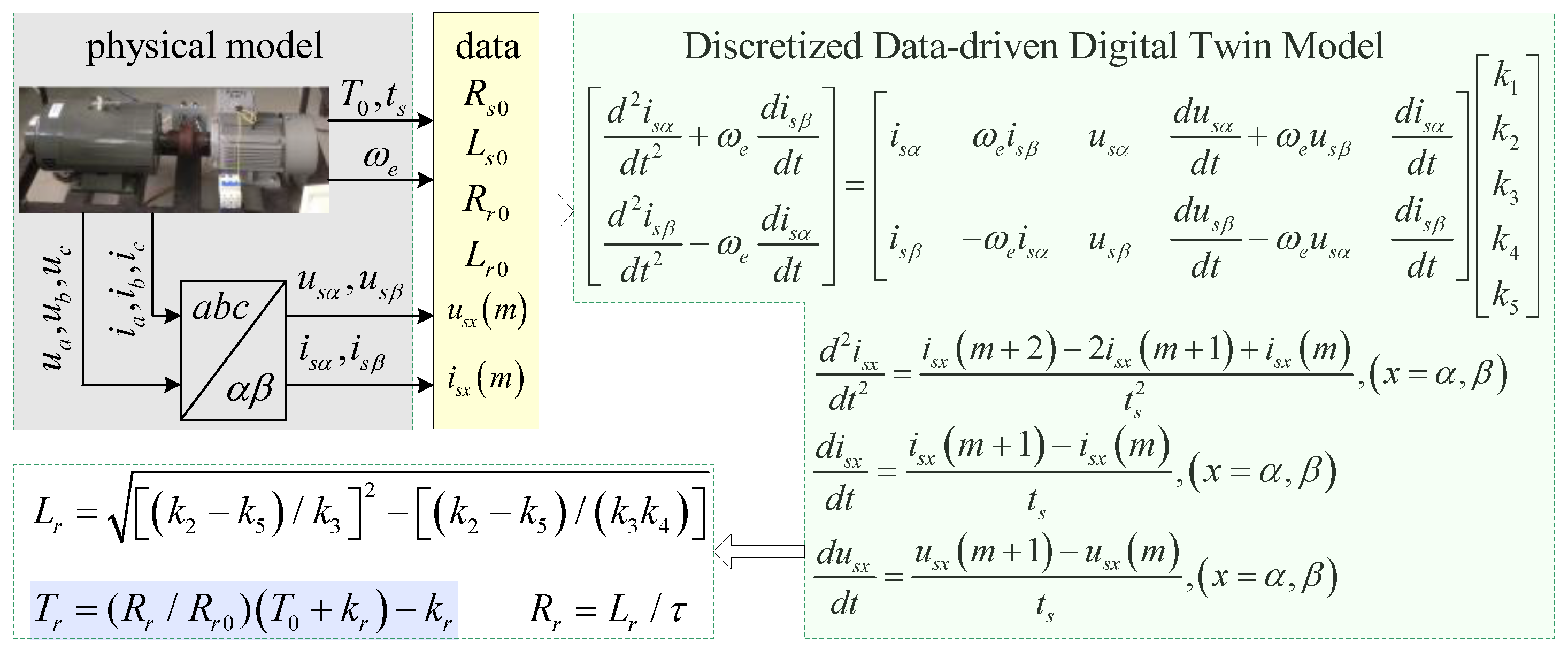
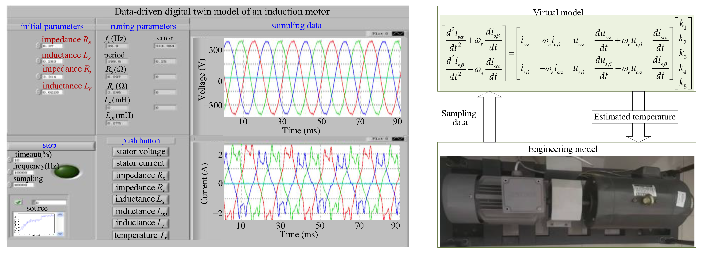
3. Data-Driven Digital Twin Model
| Algorithm 1: Algorithm of proposed data-driven digital twin model |
| 0: Modeling an induction motor by the differential equations, providing |
| 1: Call (14), and replace the differential operator with (16) |
| 2: Differential equations were transformed into algebraic equations (17) |
| 3.1: Solving characteristic algebraic equation (17) |
| 3.2: Extract accuracy fundamental voltage and current and eliminate intermediate variable based on sampling data |
| 3.3: Obtain analytic solutions , based on (21) and (22) |
| 4.1: k = 1 |
| 4.2: , calculate power factor angle , , |
| 4.3: , , |
| 4.4: Call (18) derive |
| 4.6: Call (17) and (20) obtain |
| 4.7: Call (26) and (27) calculate |
| 4.8: Obtain by calling (28) |
| 4.9: k = k + 1 and repeat above process 4.2–4.8 |
| 5.0: End |
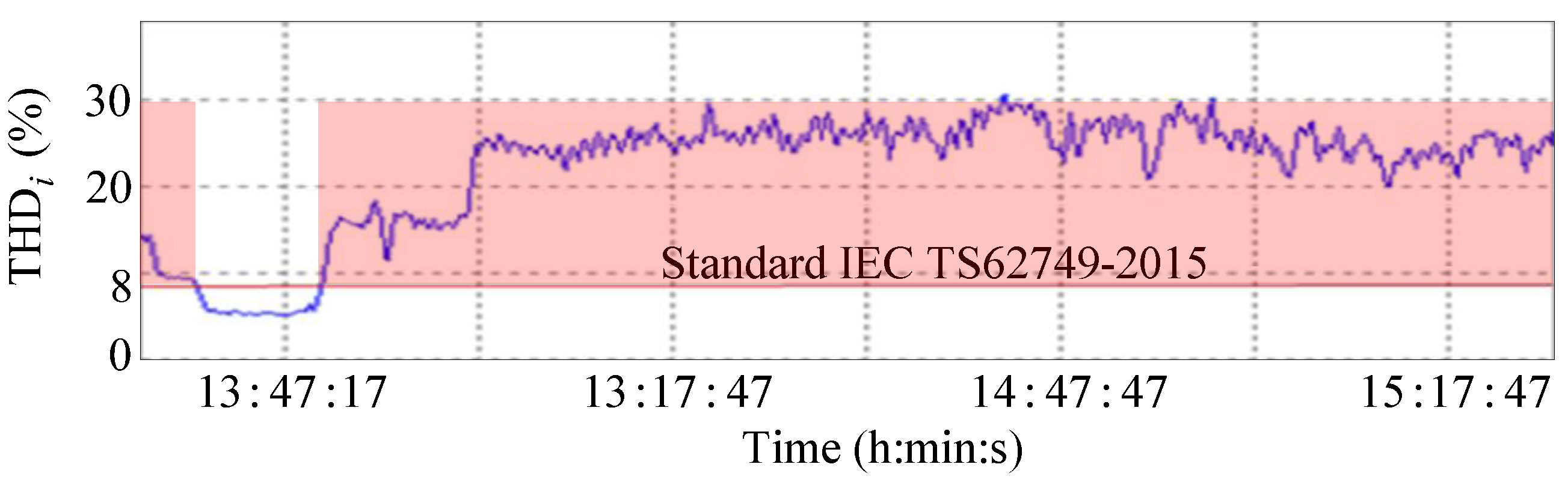
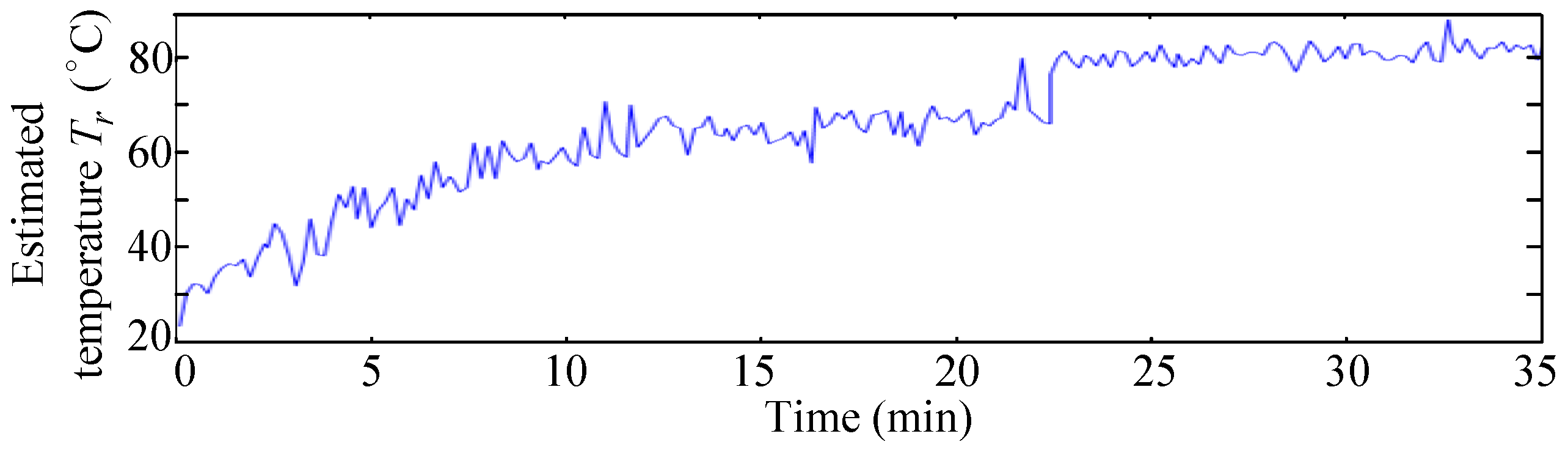
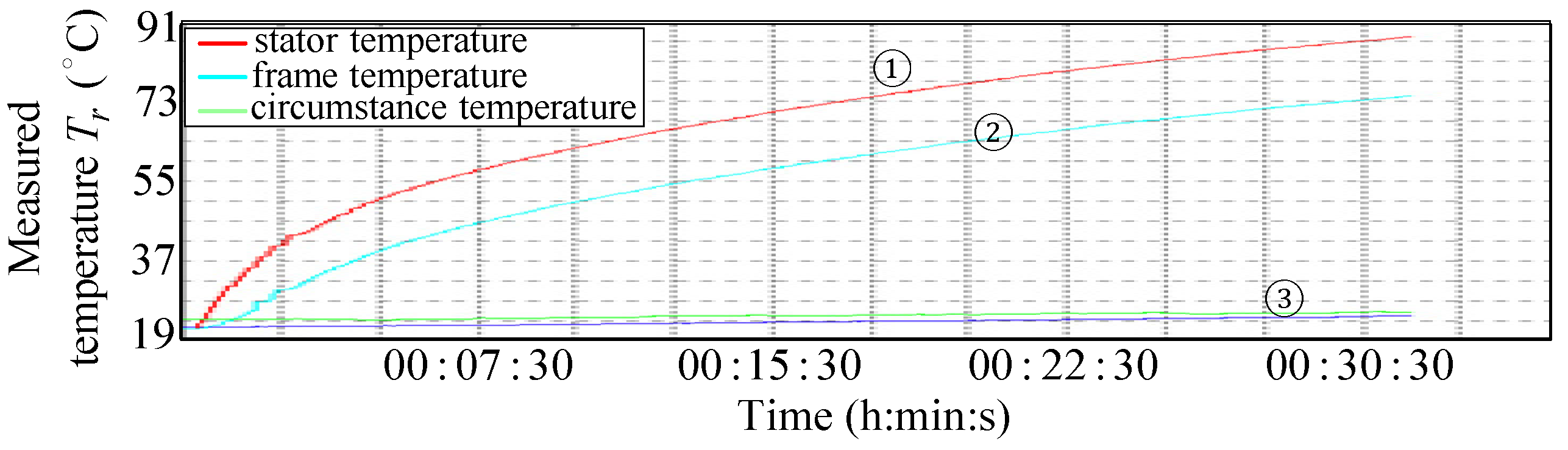
4. Experiment Validation


| Order | Part of the Experiment | Parameters | Note |
|---|---|---|---|
| 1 | (1) AC motor | 1.5 kW/AC380V | We should estimate the rotor temperature of this motor due to it being used to drive a coaxial DC motor. |
| 2 | (2) DC motor | 2.0 Hp/DC180V | It is a load generator for the AC motor. |
| 3 | (3) Inverter | 5 kW/AC380V | It is used to power the AC motor. |
| 4 | (4) Signal conditioning circuit | 0–3.3 V output voltage | 6 channels for sampling; 3 phases of voltage and 3 phases of voltage |
| 5 | (5) Power Analyzer | 3 current sensors and 3 voltage sensors | It is used to test the stator voltage and current of the AC motor |
| 6 | (6) TMP-A temperature instrument | 4 thermocouples | It is used to measure the temperature between the stator and rotor of the AC motor. |
5. Conclusions
Author Contributions
Funding
Data Availability Statement
Conflicts of Interest
Appendix A
References
- Chertovskih, R.; Pogodaev, N.; Staritsyn, M.; Aguiar, A.P. Optimal Control of Diffusion Processes: Infinite-Order Variational Analysis and Numerical Solution. IEEE Control. Syst. Lett. 2024, 8, 1469–1474. [Google Scholar] [CrossRef]
- Wu, Y.-H.; Liu, M.-Y.; Song, H.; Li, C.; Yang, X.-L. A Temperature and magnetic field-based approach for stator inter-turn fault detection. IEEE Sens. J. 2022, 22, 17799–17807. [Google Scholar] [CrossRef]
- Vitale, G.; Lullo, G.; Scire, D. Thermal Stability of a DC/DC Converter with Inductor in Partial Saturation. IEEE Trans. Ind. Electron. 2021, 68, 7985–7995. [Google Scholar] [CrossRef]
- Scirè, D.; Lullo, G.; Vitale, G. Assessment of the Current for a Non-Linear Power Inductor Including Temperature in DC-DC Converters. Electronics 2023, 12, 579. [Google Scholar] [CrossRef]
- Yamazaki, K.; Suzuki, A.; Ohto, M.; Takakura, T. Harmonic Loss and Torque Analysis of High-Speed Induction Motors. IEEE Trans. Ind. Appl. 2012, 48, 933–941. [Google Scholar] [CrossRef]
- Yamazaki, K.; Suzuki, A.; Ohto, M.; Takakura, T.; Nakagawa, S. Equivalent Circuit Modeling of Induction Motors Considering Stray Load Loss and Harmonic Torques Using Finite Element Method. IEEE Trans. Magn. 2011, 47, 986–989. [Google Scholar] [CrossRef]
- Zhang, D.; Dai, H.; Zhao, H.; Wu, T. A Fast Identification Method for Rotor Flux Density Harmonics and Resulting Rotor Iron Losses of Inverter-Fed Induction Motors. IEEE Trans. Ind. Electron. 2018, 65, 5384–5394. [Google Scholar] [CrossRef]
- Wu, C.; Nian, H.; Zhou, Q.; Cheng, P.; Pang, B.; Sun, D. Harmonic Impedance Modeling of DFIG Considering Dead Time Effect of Rotor Side Converter. In Proceedings of the 2018 IEEE Energy Conversion Congress and Exposition (ECCE), Portland, OR, USA, 23–27 September 2018; pp. 950–955. [Google Scholar]
- Pengcheng, D.; Dianguo, X.; Bo, W.; Yong, Y. Offline Parameter Identification Strategy of Permanent Magnet Synchronous Motor Considering the Inverter Nonlinearities. In Proceedings of the 2022 25th International Conference on Electrical Machines and Systems (ICEMS), Chiang Mai, Thailand, 29 November–2 December 2022; pp. 1–5. [Google Scholar]
- Yang, Y.; Zhang, G.; Zhou, Y.; Chen, B.; Ma, R.; Li, Z. A Review of Permanent Magnet Synchronous Motor Parameter Iden-tification Research. In Proceedings of the IECON 2023—49th Annual Conference of the IEEE Industrial Electronics Society, Singapore, 16–19 October 2023. [Google Scholar]
- Geravandi, M.; CheshmehBeigi, H.M. Stray Load Losses Determination Methods of Induction Motors-A Review. In Proceedings of the 2022 30th International Conference on Electrical Engineering (ICEE), Tehran, Iran, 17–19 May 2022; pp. 1033–1038. [Google Scholar]
- Ma, Z.; Zhang, W.; He, J.; Jin, H. Multi-Parameter Online Identification of Permanent Magnet Synchronous Motor Based on Dynamic Forgetting Factor Recursive Least Squares. In Proceedings of the 2022 IEEE 5th International Electrical and Energy Conference (CIEEC), Nanjing, China, 27–29 May 2022; pp. 4865–4870. [Google Scholar]
- Li, Z.; Feng, G.; Lai, C.; Li, W.; Kar, N.C. Current injection-based simultaneous stator winding and PM temperature estimation for dual three-phase PMSMs. IEEE Trans. Ind. Appl. 2021, 57, 4933–4945. [Google Scholar] [CrossRef]
- Geravandi, M.; CheshmehBeigi, H.M. Stator Windings Resistance Estimation Methods of In-Service Induction Mo-tors-A Review. In Proceedings of the 2023 31st International Conference on Electrical Engineering (ICEE), Tehran, Iran, 9–11 May 2023. [Google Scholar]
- Fang, H.; Duan, X.; Yang, Y.; Wang, Y.; Luo, G. Deadbeat Control of Permanent Magnet Synchronous Motor Based on MRAS Parameter Identification. In Proceedings of the 2020 23rd International Conference on Electrical Machines and Systems (ICEMS), Hamamatsu, Japan, 24–27 November 2020. [Google Scholar]
- Xiao, Q.; Liao, K.; Shi, C.; Zhang, Y. Parameter identification of direct-drive permanent magnet synchronous generator based on EDMPSO-EKF. IET Renew. Power Gener. 2022, 16, 1073–1086. [Google Scholar] [CrossRef]
- Zhou, S.; Wang, D.; Li, Y. Parameter identification of permanent magnet synchronous motor based on modified-fuzzy particle swarm optimization. Energy Rep. 2023, 9, 873–879. [Google Scholar] [CrossRef]
- Wu, Y.; Gao, H. Induction-motor stator and rotor winding temperature estimation using signal injection method. IEEE Trans. Ind. Appl. 2006, 42, 1038–1044. [Google Scholar]
- Jing, H.; Chen, Z.; Wang, X.; Wang, X.; Ge, L.; Fang, G.; Xiao, D. Gradient Boosting Decision Tree for Rotor Temperature Estimation in Permanent Magnet Synchronous Motors. IEEE Trans. Power Electron. 2023, 38, 10617–10622. [Google Scholar] [CrossRef]
- Chu, L.; Zhu, P.; Chang, C. Research on Full Brake-By-Wire System and Clamping Force Estimation Strategy Based on Redundant Drive Motors. IEEE Access 2023, 11, 124098–124113. [Google Scholar] [CrossRef]
- Zhao, H.; Eldeeb, H.H.; Wang, J.; Kang, J.; Zhan, Y.; Xu, G.; Mohammed, O.A. Parameter Identification Based Online Noninvasive Estimation of Rotor Temperature in Induction Motors. IEEE Trans. Ind. Appl. 2021, 57, 417–426. [Google Scholar] [CrossRef]
- Jin, L.; Wei, L.; Li, S. Gradient-based differential neural-solution to time-dependent nonlinear optimization. IEEE Trans. Autom. Control. 2023, 68, 620–627. [Google Scholar] [CrossRef]
- Ahmad, J.; Iqbal, A.; Hassan, Q.M.U. Study of nonlinear fuzzy integral differential equations using mathematical methods and applications. Int. J. Fuzzy Log. Intell. Syst. 2021, 21, 76–85. [Google Scholar] [CrossRef]
- Shams, M.; Kausar, N.; Agarwal, P.; Momani, S.; Shah, M.A. Highly efficient numerical scheme for solving fuzzy system of linear and non-linear equations with application in differential equations. Appl. Math. Sci. Eng. 2022, 30, 777–810. [Google Scholar] [CrossRef]
- Zienkiewicz, O.C.; Taylor, R.L. The Finite Element Method; Butterworth-Heinemann: Oxford, UK, 2000; Volume 2. [Google Scholar]
- Dangal, T.; Chen, C.; Lin, J. Polynomial particular solutions for solving elliptic partial differential equations. Comput. Math. Appl. 2017, 73, 60–70. [Google Scholar] [CrossRef]
- Raza, A.; Farid, S.; Amir, M.; Yasir, M.; Danyal, R.M. A study on convergence analysis of Adomian decomposition method applied to different linear and non-linear equations. Interface J. Sci. Eng. Res. 2020, 11, 1358–1378. [Google Scholar]
- Wang, B.; Duan, N.; Sun, K. A time–power series-based semi-analytical approach for power system simulation. IEEE Trans. Power Syst. 2019, 34, 841–851. [Google Scholar] [CrossRef]
- Xu, X.; Yao, R.; Sun, K.; Qiu, F. A Semi-analytical solution approach for solving constant-coefficient first-order partial differential equations. IEEE Control. Syst. Lett. 2022, 6, 704–709. [Google Scholar] [CrossRef]
- Shams, M.; Kausar, N.; Alayyash, K.; Al-Shamiri, M.M.; Arif, N.; Ismail, R. Semi-analytical scheme for solving intuitionistic fuzzy system of differential equations. IEEE Access 2023, 11, 33205–33223. [Google Scholar] [CrossRef]
- Shams, M.; Kausar, N.; Kousar, S.; Pamucar, D.; Ozbilge, E.; Tantay, B. Computationally semi-numerical technique for solving system of intuitionistic fuzzy differential equations with engineering applications. Adv. Mech. Eng. 2022, 14. [Google Scholar] [CrossRef]
- Xu, S.; Guan, X.; Peng, Y.; Liu, Y.; Cui, C.; Chen, H.; Ohtsuki, T.; Han, Z. Deep reinforcement learning based data-driven mapping mechanism of digital twin for internet of energy. IEEE Trans. Netw. Sci. Eng. 2024, 11, 3876–3890. [Google Scholar] [CrossRef]
- Chen, Z.; Liang, D.; Jia, S.; Yang, L.; Yang, S. Incipient inter-turn short-circuit fault diagnosis of permanent magnet synchronous motors based on the data-driven digital twin model. IEEE J. Emerg. Sel. Top. Power Electron. 2023, 11, 3514–3524. [Google Scholar] [CrossRef]
- Wang, T.; Chiang, H.-D. Neighboring Stable Equilibrium Points in Spatially-Periodic Nonlinear Dynamical Systems: Theory and Applications. IEEE Trans. Autom. Control. 2015, 60, 2390–2401. [Google Scholar] [CrossRef]
- Wang, L.G.; Zhang, X.; Xu, D.; Huang, W. Study of a differential control method for solving chaotic solutions of a nonlinear dynamic system. Nonlinear Dyn. 2011, 67, 2821–2833. [Google Scholar] [CrossRef]
- IEC TS62749; Assessment of Power Quality—Characteristics of Electrics Supplied by Public Networks. International Electrotechnical Commission: Geneva, Switzerland, 2015.
- IEC 60034-2-1; Standard Methods for Determining Losses and Efficiency from Tests (Excluding Machines for Traction Vehicles). International Electrotechnical Commission: Geneva, Switzerland, 2014.


| Order | Source of the Thermal | Negative Effect Analysis | Influence on Estimating Temperature | Reference |
|---|---|---|---|---|
| 1 | Harmonic current | Additional copper loss of stator and rotor | 1. Influence on the normal change rule of temperature with the stator current. 2. Causing irregular changes in the inductance and resistance of the induction motor. | [5] |
| Stray loss of stator and rotor | [6] | |||
| Additional iron loss of stator | [7] | |||
| Increase the impedance of the rotor | [8] |
| Order | Methods | Advantages | Disadvantages | References |
|---|---|---|---|---|
| 1 | Recursive Least Squares (RLS) | The algorithm is simple | the problem of data saturation | [9,10] |
| 2 | Stator windings resistance (SWR) measurement | It is entirely accurate and is used as a reference for measuring the precision. | 1. SWR measurement is highly intrusive. 2. SWR measurement requires turning off the IM and disconnecting the IM supply connections. | [11] |
| 3 | IM dynamic model-based SWR | 1. The method is non-intrusive. 2. Can be used in thermal monitoring and IM protection programs. | 1. The need to know the values of IM dynamic model parameters for SWR estimation. 2. Less accuracy in SWR estimation at speeds other than low speed. 3. Intense sensitivity to changes in IM dynamic model parameters. | [12] |
| 4 | DC signal injection-based SWR | 1. For SWR estimation, there is no need to know the values of the IM dynamic model parameters. 2. Can be used in thermal monitoring and IM protection programs. 3. The method has a high level of accuracy. | 1. The need for an additional circuit to inject the DC signal in the line-fed IMs. 2. Unbalance in IM feeding due to additional signal injection. 3. The presence of ripple in the IM torque. | [13,14] |
| 5 | Model Reference Adaptive System (MRAS) | The algorithm is simple | It is suitable for the problem of poor order | [15] |
| 6 | Extended Kalman Filter (EKF) algorithm | Noise impact is small | The algorithm is complex, with poor robustness | [16] |
| 7 | Intelligent algorithms | Good search ability, strong global search capability | The algorithm is complex and easy to fall into local optimum | [17] |
| 8 | Proximal Policy Optimization-Reinforcement Learning (PPO-RL) algorithm | The algorithm is stable and computationally efficient | The algorithm is sample-inefficient and cannot be run online | [18] |
| 9 | Machine learning method | The algorithm can effectively predict motor temperature. | The algorithm is offline, with poor applicability | [19,20] |
| 10 | Combination parameter identification method | This approach combines the advantages of Recursive Least Squares (RLS) and the Model Reference Adaptive System (MRAS). | The algorithm is complex and hard to realize online. | [21] |
| Order | Methods | Advantages | Disadvantages | References | |
|---|---|---|---|---|---|
| 1 | Numerical methods | Gradient-based differential neural solutions | The essence of these methods is iterative calculation, which is suitable to solve any differential equations. | It can be derived from the analytical solution of a differential equation directly and online. | [22] |
| Nonlinear fuzzy method | [23] | ||||
| Highly efficient numerical scheme | [24] | ||||
| Finite element method | [25] | ||||
| Polynomial particular solutions method | [26] | ||||
| Adomian decomposition method | [27] | ||||
| 2 | Semi-analytical methods | semi-analytical solution approach | By these methods, approximate analytical solutions can be obtained. | It is difficult to obtain an online analytical solution to a differential equation in on-chip system. | [28,29] |
| semi-analytical scheme | [30] | ||||
| computational semi-numerical technique | [31] | ||||
| Order | Parameters | Unit | Note |
|---|---|---|---|
| 1 | , | A | Stator currents of the induction motor in coordinate system |
| 2 | , | V | Stator voltage of the induction motor in coordinate system |
| 3 | Wb | Stator flux of the induction motor in coordinate system | |
| 4 | / | Ω/H | Stator impedance/inductance of the induction motor |
| 5 | / | Ω/H | Rotor impedance/inductance of the induction motor |
| 6 | H | Mutual/leakage inductance of the induction motor | |
| 7 | H | Leakage inductance of the motor, | |
| 8 | s | Time constant of the motor rotor, | |
| 9 | rad/s | Power supply angular frequency | |
| 10 | Variable , | ||
| 11 | s | Sampling period | |
| 12 | , | V/A | Sampling voltage and current at kth period in axis and axis, respectively, where |
| 13 | °C | The ambient temperature of the induction motor | |
| 14 | Ω | Initial impedance of the stator of the motor under T0 | |
| 15 | The impedance coefficient of the induction motor | ||
| 16 | °C | The rotor temperature of the induction motor | |
| 17 | V/A | The sampling voltage and current of the motor stator | |
| 18 | ° | Phase difference between the sampling and the | |
| 19 | V | Positive sequence voltage , | |
| 20 | The resistance constant of the induction motor | ||
| 21 | Voltage and current in coordinate system, where | ||
| 22 | |||
| 23 | The coefficient of correction |
| Order | Main Steps |
|---|---|
| 1 | Algebraization of the differential equations: substitute the differential operator by the quotient of two adjacent sampling data and the sampling period. |
| 2 | Solving the equivalent algebraic equations: to derive the expression regarding the rotor temperature by solving approximate algebraic difference equations. |
| 3 | Repeat the above procedures at every sampling period. |
| Data | Error | |||
|---|---|---|---|---|
| Term | ||||
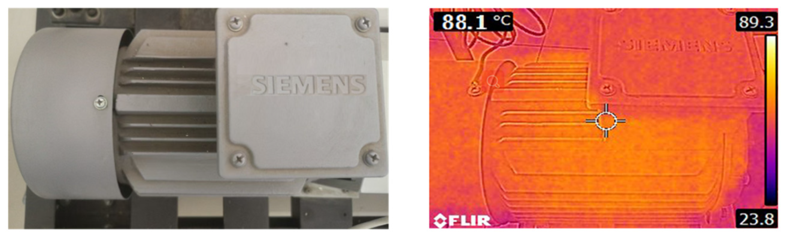
| End time | 89.6 | 88.0 | 1.8% | |
| Start time | 23.3 | 23.0 | 1.3% | |
Disclaimer/Publisher’s Note: The statements, opinions and data contained in all publications are solely those of the individual author(s) and contributor(s) and not of MDPI and/or the editor(s). MDPI and/or the editor(s) disclaim responsibility for any injury to people or property resulting from any ideas, methods, instructions or products referred to in the content. |
© 2024 by the authors. Licensee MDPI, Basel, Switzerland. This article is an open access article distributed under the terms and conditions of the Creative Commons Attribution (CC BY) license (https://creativecommons.org/licenses/by/4.0/).
Share and Cite
Luo, Y.; Wang, L.; Sidorov, D.; Dreglea, A.; Chistyakova, E. An Approach to Estimate the Temperature of an Induction Motor under Nonlinear Parameter Perturbations Using a Data-Driven Digital Twin Technique. Energies 2024, 17, 4996. https://doi.org/10.3390/en17194996
Luo Y, Wang L, Sidorov D, Dreglea A, Chistyakova E. An Approach to Estimate the Temperature of an Induction Motor under Nonlinear Parameter Perturbations Using a Data-Driven Digital Twin Technique. Energies. 2024; 17(19):4996. https://doi.org/10.3390/en17194996
Chicago/Turabian StyleLuo, Yu, Liguo Wang, Denis Sidorov, Aliona Dreglea, and Elena Chistyakova. 2024. "An Approach to Estimate the Temperature of an Induction Motor under Nonlinear Parameter Perturbations Using a Data-Driven Digital Twin Technique" Energies 17, no. 19: 4996. https://doi.org/10.3390/en17194996