Relevance-Based Reconstruction Using an Empirical Mode Decomposition Informer for Lithium-Ion Battery Surface-Temperature Prediction

Abstract

Accurate monitoring of lithium-ion battery temperature is essential to ensure these batteries’ efficient and safe operation. This paper proposes a relevance-based reconstruction-oriented EMD-Informer machine learning model, which combines empirical mode decomposition (EMD) and the Informer framework to estimate the surface temperature of 18,650 lithium-ion batteries during charging and discharging processes under complex operating conditions. Initially, based on 9000 data points from the U.S. NASA Prognostics Center of Excellence’s random battery-usage dataset, where each data point includes three features: temperature, voltage, and current, EMD is used to decompose the temperature data into intrinsic mode functions (IMFs). Subsequently, the IMFs are reconstructed into low-, medium-, and high-correlation components based on their correlation with the original data. These components, along with voltage and current data, are fed into sub-models. Finally, the model captures the long-term dependencies among temperature, voltage, and current. The experimental results show that, in single-step prediction, the mean squared error, mean absolute error, and maximum absolute error of the model’s predictions are 0.00095, 0.02114, and 0.32164 °C; these metrics indicate the accurate prediction of the surface temperature of lithium-ion batteries. In multi-step predictions, when the prediction horizon is set to 12 steps, the model achieves a hit rate of 93.57% where the maximum absolute error is within 0.5 °C; under these conditions, the model combines high predictive accuracy with a broad predictive range, which is conducive to the effective prevention of thermal runaway in lithium-ion batteries.

1. Introduction

Lithium-ion batteries, due to their high energy density, long service life, and low self-discharge rate, have gained widespread application in electric vehicles, energy storage systems, and other fields [1]. The optimal operating temperature range for lithium-ion batteries is 20 °C to 40 °C [2]. If the battery materials continuously remain within abnormal temperature ranges, this can lead to accelerated degradation of the positive and negative electrode materials, electrolyte decomposition, and increased internal resistance, resulting in increased heat generation [3]. If cooling is inadequate and temperature rise is uncontrolled, it may trigger a thermal runaway process [4]. With the expansion of the new energy industry, incidents of fires are increasing, and over 90% of these incidents are attributed to thermal runaway of batteries [5]. As shown in Figure 1, constructing an accurate lithium-ion battery temperature prediction model can reveal future surface temperature trends. If the residuals between the predicted and actual values exceed a threshold, it indicates potential anomalies in the battery [6], and the battery’s operating state can be adjusted in advance based on the warning information to effectively prevent thermal runaway [7].

Currently, battery temperature prediction models can be categorized into two types: physical models [8] and data-driven models [9]. Physical models are constructed based on the electrochemical mechanisms or external electrical behavior of batteries, such as electrochemical models and equivalent circuit models (ECMs) [10]. To ensure the accuracy of these models, it is necessary to consider the coupled relationships among the battery’s structure, size, materials, temperature, and usage scenarios [11]. Sun et al. [12] combined a first-order ECM with an Extended Kalman Filter to establish a real-time temperature-estimation model; however, they overlooked the impact of battery temperature on model parameters. The equivalent resistance and capacitance values change with temperature variations, which in turn affect the accuracy of the model. Liu et al. [13] established a temperature prediction model by combining a two-state thermal model with a second-order ECM; however, the model exhibits instability during current and voltage-step changes, which may lead to divergence in the identification results. In contrast, machine learning algorithms can identify complex nonlinear relationships and latent variables in the data. Data-driven models, which rely entirely on external data and do not require consideration of intricate internal battery structures or parameters, often achieve high precision [14]. The model has advantages in terms of generality and portability. Álvarez Antón et al. [15] proposed a support vector machine (SVM) model that can be implemented in microcontroller-based battery management systems (BMSs). Guo et al. [16] developed an improved back-propagation (BP) neural network using battery current, voltage, and ambient temperature as inputs. This model has a fast computation speed and significantly reduces the state of charge (SOC) prediction error in practical applications. Therefore, data-driven models are very suitable for online prediction in the context of BMS [17]. Wang et al. [18] established a temperature prediction model for lithium-ion batteries using a local regression neural network, demonstrating shorter training times and better adaptability and generalization capabilities. Jiang et al. [19] employed long short-term memory (LSTM) recurrent neural networks and gated recurrent unit (GRU) recurrent neural networks to predict the surface temperature of 18,650 lithium-ion batteries under different environmental temperatures, proposing the use of temperature differences along the time axis as the output of the neural network, which aligns well with electrochemical and thermodynamic principles. Jiang et al. [20] combined an elitist preservation genetic algorithm with bidirectional LSTM neural networks, using an improved loss function to achieve precise prediction of upper and lower temperature limits.

In previous studies, the training data for models primarily originated from experimental results under periodic operating conditions or single charge–discharge cycles, which made it difficult for the models to accurately capture the nonlinear temperature dynamics exhibited by batteries under complex operating conditions, potentially reducing prediction accuracy. Moreover, most of these models have focused on improving single-step-ahead prediction accuracy, and thus lack a broad prediction range.

This paper utilizes the RW10 dataset from NASA’s Prognostics Center of Excellence [21], which contains 9000 sets of random usage data for 18,650 lithium-ion batteries. Each set includes three features: temperature, voltage, and current. In practical applications, these data can be obtained through corresponding sensors. On this basis, EMD was introduced as a method for processing nonlinear and nonstationary signals. EMD decomposes the temperature data into a series of IMFs. Pearson correlation coefficients (PCCs) were then used to measure the strength of correlation between continuous variables. IMFs with low correlation represent noise or high-frequency disturbances in the temperature data; IMFs with medium correlation characterize the mid-frequency features of the temperature data, and IMFs with high correlation represent the long-term trends or dominant periodicities in the temperature data. These components were combined with voltage and current data and input into sub-models. Ultimately, the model captures the long-term dependencies among temperature, voltage, and current, achieving accurate temperature prediction under complex operating conditions. Additionally, this study employed the Informer framework, which implements a probabilistic sparse self-attention mechanism by focusing on the most informative query vectors. This approach reduces computational complexity while achieving high-precision predictions. Based on this framework, single-step and multi-step predictions of the surface temperature of lithium-ion batteries were conducted, thereby enhancing the range of temperature predictions under complex operating conditions.

2. Surface Temperature Prediction Model

2.1. The Empirical Mode Decomposition

The core idea of EMD is to iteratively decompose the data from high frequency to low frequency into a series of IMFs and a residual component, according to the local temporal feature scale of the data, so as to achieve noise reduction and smoothing of the data [22]. The detailed decomposition steps are shown in Figure 2.

Through iterative decomposition from high to low frequency, multiple IMF components can be obtained. Time series $x\left(t\right)$ can be expressed by EMD as follows:

$$x\left(t\right)={\displaystyle {\sum }_{f=1}^{m}im{f}_f\left(t\right)+r\left(t\right)}$$

(1)

where m represents the number of $im{f}_f\left(t\right)$, $im{f}_f\left(t\right)$ represents the intrinsic mode function of $x\left(t\right)$, and $r\left(t\right)$ represents the residual term.

2.2. The Informer Framework

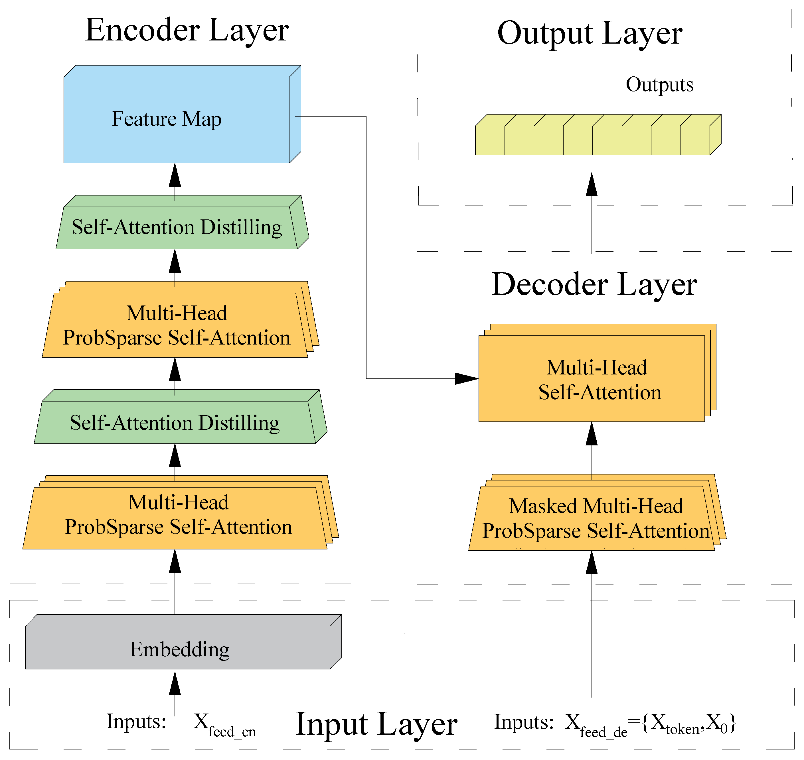
As an efficient improvement of the traditional Transformer [23], the Informer primarily addresses the efficiency and performance issues encountered when processing long sequences through the introduction of the ProbSparse Self-Attention mechanism; this mechanism enables the Informer to maintain excellent performance while significantly reducing the demand for computational resources. As shown in Figure 3, the Informer framework is primarily divided into the input layer, Encoder layer, Decoder layer, and output layer.

2.2.1. Input Layer

The input for the Informer framework can be divided into input $X_{feed\_en}$ for the Encoder and input $X_{feed\_de}=\{X_{token},X_0\}$ for the Decoder, which are defined as follows:

$$X_{feed\_en}=[x_1,x_2,x_3,\dots ,x_u]$$

(2)

$$X_{feed\_de}=[x_1,x_2,\dots ,x_v,0,0\dots 0]$$

(3)

where u represents the length of the input sequence and v represents the length of the token. The input sequence for the Decoder is composed of two parts: first, a sequence of tokens of length v representing historical data; second, placeholders represented by 0 generated through a masking mechanism, with a length equal to the length of the sequence to be predicted.

Embedding: In the Informer framework, the inputs to both the Encoder and Decoder include three components: projection scalars, local timestamps, and global timestamps. These components are used to project multi-dimensional data from a given time point into 512-dimensional data. The values obtained from each component are combined and used as the input to the network. The formula is as follows:

$$X_{feed\left[i\right]}^{\mathrm{t}}=\alpha u_i^t+P{E}_{\left(L_x\times \left(t-1\right)+i\right)}+{\displaystyle {\sum }_p{\left[S{E}_{\left(L_x\times \left(t-1\right)+i\right)}\right]}_p}$$

(4)

where $\alpha u_i^t$ represents the projected scalar of the input sequence after one-dimensional convolution. α represents a factor that balances the size between scalar projection and local/global embeddings. If the sequence input has already been standardized, then α = 1. ${\displaystyle {\sum }_p{\left[S{E}_{\left(L_x\times \left(t-1\right)+i\right)}\right]}_p}$ represents the global timestamp, and $P{E}_{\left(L_x\times \left(t-1\right)+i\right)}$ represents the positional timestamp. The formula for calculating the positional timestamp is as follows:

$$\left\{\begin{array}{l}P{E}_{(pos,2i)}=\sin (pos/2L_x^{2i/d})\\ P{E}_{(pos,2i+1)}=\cos (pos/2L_x^{2i/d})\end{array}\right\}$$

(5)

where pos represents the position of a data instance in the input sequence, L_x represents the length of the sequence, 2i represents an even-numbered dimension, and 2i + 1 represents an odd-numbered dimension.

2.2.2. Encoder Layer

The Encoder layer is used to efficiently and sufficiently encode the input long sequence data to capture long-term dependencies and feature information across multiple time scales. Unlike the Transformer, the Informer employs a new EncoderStack structure, which is composed of multiple encoder layers and distillation layers. This structure includes ProbSparse Self-Attention and Self-Attention Distilling.

ProbSparse Self-Attention: The ProbSparse Self-Attention mechanism decides which positions require attention computation by introducing sparsity into the traditional attention mechanism. The formula for the traditional attention mechanism is as follows:

$$A\left(Q,K,V\right)=softmax\left({\displaystyle \frac{Q{K}^T}{\sqrt{d}}}\right)V$$

(6)

where Q represents the query vector that needs to be attended to and matched, K represents the feature vector in the input sequence, V represents the value vector that is weighted and output, d represents the dimension of K, and softmax () represents the activation function that converts the output values into a probability distribution. The elements within the Q and K vectors can be denoted as q and k, respectively. During the computation of $Q{K}^T$, each q is used to form a dot product with each k, and these operations are referred to as dot product pairs. The result of the dot product pairs represents the attention weights between them.

In the attention mechanism, a few key dot product pairs contribute the critical attention [24]. The q in these key dot product pairs is considered ‘active q,’ while the rest is considered ‘inactive q.’ The formula for determining whether q is active is as follows:

$$M\left(q_s,K\right)=\ln {\displaystyle {\sum }_{j=1}^d{e}^{\frac{q_s{k}_j^T}{\sqrt{d}}}}-{\displaystyle \frac{1}{d}}{\displaystyle {\sum }_{j=1}^d\frac{q_s{k}_j^T}{\sqrt{d}}}$$

(7)

where $q_s$ represents the s-th element in Q. The first term on the right-hand side of the equation is the function of the Log-Sum-Exp (LSE) of the dot products between $q_s$ and all k, and the second term is the arithmetic mean function. A large value of $M\left(q_s,K\right)$ indicates a high probability that $q_s$ will become a dominant dot product pair in the self-attention distribution. The formula for ProbSparse Self-Attention is as follows:

$$A\left(Q,K,V\right)=Softmax\left({\displaystyle \frac{\overline{Q}{K}^T}{\sqrt{d}}}\right)V$$

(8)

where $\overline{Q}$ represents the set of the most active q values.

Self-Attention Distilling: This mechanism refines knowledge from multiple attention layers into a single attention layer within the Encoder, enhancing the model’s performance by capturing different representations from various attention layers. Dimensionality reduction is achieved by adding 1D convolution and max-pooling operations after each attention block. The Informer uses Self-Attention Distilling in the Encoder module to extract the most important attention information and reduce the memory and time required by the algorithm. The formula is as follows:

$$X_{j+1}^t=Maxpool\left(ELU\left(Convld\left({\left[X_j^t\right]}_{AB}\right)\right)\right)$$

(9)

where [] represents the attention blocks, one-dimensional convolution (Conv1d) uses the ELU activation function to perform a one-dimensional convolutional filtering operation along the time dimension, and the sequence length is halved through a max-pooling layer with a stride of 2, thus reducing the overall memory usage.

2.2.3. Decoder Layer

The input of the Decoder consists of a rolling sequence segment. This sequence is first processed through a masked multi-head ProbSparse Self-Attention block. Then, it is combined with the Encoder output and serves as an input to the unmasked multi-head self-attention module. Finally, the output is passed through a fully connected layer to obtain the prediction results.

2.2.4. Output Layer

The output of the Informer contains only the target sequence, i.e., the predicted values, without any auxiliary information. Unlike the Transformer, the Informer generates the entire prediction sequence in one step rather than inferring each prediction value sequentially. This approach reduces cumulative error during the prediction process and improves prediction efficiency.

2.3. The EMD-Informer Model

2.3.1. Data Processing

To simplify the prediction model, we reconstructed $im{f}_f\left(t\right)$ and $r(t)$ into three components based on their PCCs: low-, medium-, and high-correlation components. Let $x\left(t\right)$ = X, $\left\{im{f}_1(t),im{f}_2(t)\dots im{f}_m(t),r(t)\right\}=Y$. The formula for calculating the PCC is as follows [25]:

$$R={\displaystyle \frac{{\displaystyle {\sum }_{t=1}^l\left(X_t-\overline{X}\right)}\left(Y_t-\overline{Y}\right)}{\sqrt{{\displaystyle {\sum }_{t=1}^l{\left(X_t-\overline{X}\right)}^2}}\sqrt{{\displaystyle {\sum }_{t=1}^l{\left(Y_t-\overline{Y}\right)}^2}}}}$$

(10)

where R represents the Pearson correlation values, l is the dimension of X and Y, $X_t$ and $Y_t$ are the t-th elements in X and Y, respectively, and $\overline{X}$ and $\overline{Y}$ are the means of X and Y, respectively.

We used the method of mean plus or minus the standard deviation to identify values that are far from the mean. The formula is as follows:

$$\overline{R}={\displaystyle \frac{{\displaystyle {\sum }_{a=1}^{m+1}{R}_a}}{m+1}}$$

(11)

$$T=\overline{R}\pm \sqrt{{\displaystyle \frac{{\displaystyle {\sum }_{a=1}^{m+1}{\left(R_a-\overline{R}\right)}^2}}{m+1}}}$$

(12)

where $\overline{R}$ represents the mean correlation, T represents the correlation threshold, and $R_a$ is the a-th correlation coefficient in R. Based on T, the correlation coefficients are divided into three intervals: low correlation, medium correlation, and high correlation. The IMFs corresponding to the correlation coefficients within each interval are summed and reconstructed. If there are N IMFs within an interval, then

$$H_{sum}={\displaystyle {\sum }_{b=1}^N{H}_b}$$

(13)

where $H_{sum}$ represents the summed and reconstructed component and $H_b$ is the b-th IMF component within the interval.

The temperature prediction model consists of three Informer sub-models. After the reconstruction of IMFs within three intervals, the low-, medium-, and high-correlation components are fed as inputs to sub-models 1, 2, and 3, respectively.

2.3.2. The EMD-Informer Model Architecture

As illustrated in Figure 4, the main steps of the EMD-Informer model are as follows:

• Use EMD to decompose the temperature data into several IMFs;
• Calculate the PCC between the IMFs and the original temperature data, and reconstruct the IMFs into low-, medium-, and high-correlation components based on the level of correlation;
• The reconstructed components with different correlation degrees, along with the feature data of current and voltage, are used as inputs for the sub-models;
• Calculate the outputs of the sub-models and reconstruct them to obtain the final prediction output.

3. Dataset and Evaluation Metrics

3.1. Dataset

The charging and discharging strategy for the battery cycles in the RW10 dataset is a random walk strategy: the charging and discharging currents are randomly selected from the set {−4.5 A, −3.75 A, −3 A, −2.25 A, −1.5 A, −0.75 A, 0.75 A, 1.5 A, 2.25 A, 3 A, 3.75 A, 4.5 A}. Negative currents represent charging, while positive currents represent discharging. During battery operation, a selected current setting is applied until the terminal voltage exceeds the range of 3.2 V to 4.2 V, or until a specific charge–discharge condition persists for five minutes. After each charging or discharging period, there is a rest period of less than one second during which the current is 0 while a new charging or discharging current setpoint is selected. The current probabilities are shown in Figure 5. From the RW10 dataset, a subset of 9000 data groups was selected for analysis, with each group containing temperature, voltage, and current data. The first 80% of the data are used for training, and the remaining 20% are used for testing. The relationship between battery temperature and voltage and current is shown in Figure 6.

3.2. Evaluation Criteria

To quantitatively assess performance, the mean squared error (MSE), mean absolute error (MAE), and maximum absolute error (MAXE) were selected as the evaluation metrics for assessing model performance. The evaluation metrics are defined as follows:

$$MSE={\displaystyle \frac{1}{n}}{\displaystyle {\sum }_{i=1}^n{\left({\widehat{y}}_i-y_i\right)}^2}$$

(14)

$$MAE={\displaystyle \frac{1}{n}}{\displaystyle {\sum }_{i=1}^n\left|{\widehat{y}}_i-y_i\right|}$$

(15)

$$MAXE=Max\left|{\widehat{y}}_i-y_i\right|$$

(16)

where $y_i$ represents the true value of the i-th temperature point, ${\widehat{y}}_i$ represents the model’s prediction for the i-th temperature point, and n represents the number of test sample data points.

4. Experimental Analysis

4.1. Model Training and Parameter Optimization

According to Equation (10), the correlation values between $im{f}_f\left(t\right)$, $r(t)$, and the original series are calculated as shown in

Table 1. Correlation values between modal functions and the original sequence.

Parameter	PCC
$im{f}_1(t)$	−0.01238
$im{f}_2(t)$	0.00190
$im{f}_3(t)$	0.03288
$im{f}_4(t)$	0.12448
$im{f}_5(t)$	0.21860
$im{f}_6(t)$	0.37338
$im{f}_7(t)$	0.49136
$im{f}_8(t)$	0.45558
$im{f}_9(t)$	0.45950
$im{f}_{10}(t)$	0.23390
$r(t)$	0.23561

.

According to Equations (11) through (13), the $im{f}_f\left(t\right)$ and $r(t)$ are reconstructed into low-, medium-, and high-correlation components. These components, combined with the voltage and current feature data, are used as inputs for sub-models 1, 2, and 3, respectively.

This paper optimizes the parameters for single-step prediction of the three sub-models by adjusting the model dimensions and batch sizes. Each sub-model is trained for 10 epochs. The optimization process involves inputting batch sizes of 16, 32, and 64, and model dimensions of 256, 512, and 1024. After multiple experiments, the optimal values are selected. The optimization results are shown in

Table 2. The results of the model optimization.

Dimension of Model		256			512			1024
Batch Size		16	32	64	16	32	64	16	32	64
Sub-model 1	MSE	0.00080	0.00080	0.00081	0.00077	0.00080	0.00080	0.00080	0.00076	0.00085
	MAE	0.01588	0.01614	0.01625	0.01547	0.01619	0.01607	0.01617	0.01602	0.01720
	MAXE	0.34059	0.35343	0.34334	0.34732	0.32537	0.35882	0.32567	0.31090	0.33378
Sub-model 2	MSE	0.00045	0.00095	0.00090	0.00047	0.00069	0.00086	0.00032	0.00077	0.00097
	MAE	0.01542	0.02306	0.02151	0.01640	0.02018	0.02109	0.01345	0.02179	0.02400
	MAXE	0.10481	0.13279	0.14734	0.08276	0.11686	0.14080	0.07268	0.09697	0.11312
Sub-model 3	MSE	0.00049	0.00065	0.00125	0.00061	0.00030	0.00073	0.00051	0.00038	0.00094
	MAE	0.01567	0.02013	0.02612	0.02039	0.01395	0.02146	0.01853	0.01625	0.02406
	MAXE	0.11184	0.12009	0.15740	0.09903	0.08033	0.14252	0.06930	0.06121	0.12526

.

Table 2 illustrates the following:

• For sub-model 1, the optimal model dimension and batch size for the evaluation metrics are 1024 and 32, respectively;
• For sub-model 2, the optimal model dimension and batch size for the evaluation metrics are 1024 and 16, respectively;
• For sub-model 3, the optimal model dimension and batch size for the evaluation metrics are 512 and 32, respectively;

The final selected model input parameters are shown in

Table 3. Sub-model input parameters.

Parameters	Sub-Model 1	Sub-Model 2	Sub-Model 3
Input Sequence Length	14
Start Token Length	7
Prediction Sequence Length	1
Factor	5
Numbers of Heads	8
Encoder Layers Number	2
Decoder Layers Number	1
Dimension of fcn in Model	2048
Dropout	0.05
Learning Rate	0.00005
Batch Size	32	16	32
Dimension of Model	1024	1024	512

. The evaluation error metrics for the optimal structure obtained using the parameters in Table 3 are presented in

Table 4. Evaluation of the sub-model and reconstruction results under optimal input parameters.

Method	Sub-Model 1	Sub-Model 2	Sub-Model 3	Reconstructed
MSE	0.00076	0.00032	0.00030	0.00095
MAE	0.01602	0.01345	0.01395	0.02114
MAXE	0.31090	0.07268	0.08033	0.32165

.

Table 4 illustrates that the MSE, MAE, and MAXE of the reconstructed prediction results are 0.00095, 0.02114, and 0.32165, respectively. The individual sub-models and the reconstructed prediction results are shown in Figure 7.

Figure 7a–c illustrate that three sub-models capture the data variation trends well under single-step prediction. Figure 7d illustrates that the reconstructed prediction values and the true values are nearly perfectly aligned, achieving high prediction accuracy.

4.2. Lithium-Ion Battery Surface Temperature Prediction Comparison Analysis

In this section, to validate the performance of the model proposed in this paper, experiments were conducted by comparing it with GRU, LSTM, and Informer, using the same dataset. The prediction results and absolute errors of each model are compared in Figure 8, and the evaluation metrics of each model are compared in

Table 5. Comparison of evaluation indicators of each model.

Method	LSTM	GRU	Informer	EMD–Informer
MSE	0.00537	0.00393	0.00262	0.00095
MAE	0.05286	0.05261	0.04028	0.02114
MAXE	0.49210	0.39832	0.36686	0.32164

.

Figure 8 and Table 5 illustrate that the EMD-Informer model has the smallest prediction error, with a maximum error of only 0.32164 °C, accurately predicting the trend in temperature changes.

Compared to LSTM, GRU, and the single Informer models, the EMD-Informer model shows improvements in the evaluation metrics:

• MSE is reduced by 82.31%, 75.83%, and 63.74%, respectively;
• MAE is reduced by 60.01%, 59.82%, and 47.52%, respectively;
• MAXE is reduced by 34.64%, 19.25%, and 12.33%, respectively.

4.3. Multi-Step Prediction of Battery Surface Temperature

When the prediction horizons are set to 24, 18, 12, and 6, the absolute errors of the EMD-Informer model predictions are shown in Figure 9.

Figure 9 illustrates that the absolute errors of the multi-step prediction results are generally within 1 °C. As the prediction horizon shortens, the prediction errors tend to decrease. The frequency distribution of the maximum prediction errors is shown in Figure 10.

Figure 10 illustrates that the distribution of the maximum error frequency for the predicted temperatures shows a bimodal pattern, with the two peaks located on either side of zero maximum error, indicating that the predicted values fluctuate around the true values. As the prediction horizon decreases, the bimodal phenomenon becomes less pronounced, and the frequency distribution of the maximum errors tends to cluster around 0, indicating a reduction in the maximum error and an improvement in overall prediction accuracy. The maximum absolute errors in temperature prediction for the four models over multiple prediction horizons are summarized in

Table 6. Statistical analysis of the maximum absolute error for multi-step predictions.

Error Range	Maximum Absolute Error < 1 °C				Maximum Absolute Error < 0.5 °C
Prediction Horizons	24	18	12	6	24	18	12	6
EMD-Informer hit rate	98.98%	99.40%	99.64%	100%	78.43%	84.32%	93.57%	98.32%
Informer hit rate	97.48%	98.74%	99.46%	99.92%	72.89%	81.81%	92.28%	96.82%
LSTM hit rate	97.35%	98.68%	99.22%	99.82%	74.80%	81.60%	91.27%	96.69%
GRU hit rate	95.97%	98.32%	99.28%	99.94%	65.17%	80.63%	91.15%	97.42%

.

Table 6 illustrates that the hit rate of the EMD-Informer model is higher than that of the comparative models. The hit rates of the four models decrease as the prediction horizon increases, indicating a negative correlation between high predictive accuracy and a broad predictive range. When limiting the maximum absolute error of predicted temperatures to within 1 °C, the EMD-Informer model achieves hit rates above 97% across all horizons. When the maximum absolute error is restricted to within 0.5 °C, the hit rates of the EMD-Informer model at prediction horizons of 24, 18, 12, and 6 steps are 78.43%, 84.32%, 93.57%, and 98.32%, respectively. Notably, there is a significant decrease of 9.25% in the hit rate when the prediction horizon increases from 12 to 18 steps. Considering the effective prevention of thermal runaway in lithium-ion batteries, a prediction horizon of 12 steps provides both a broader predictive range and a high hit rate.

5. Conclusions

This paper proposes a lithium-ion battery surface temperature prediction method based on the EMD-Informer model with correlation-based reconstruction, and compares it with GRU, LSTM, and single Informer prediction models. The following conclusions can be drawn:

(1)

Under complex operating conditions, changes in the surface temperature of the battery exhibit high nonlinearity. The original temperature data were decomposed using the EMD algorithm and then reconstructed into features with varying correlation degrees. These features were combined with voltage and current data to serve as inputs for the sub-models, enabling them to learn from diverse characteristics. Single-step predictions indicate that the EMD–Informer model demonstrates higher predictive accuracy.

(2)

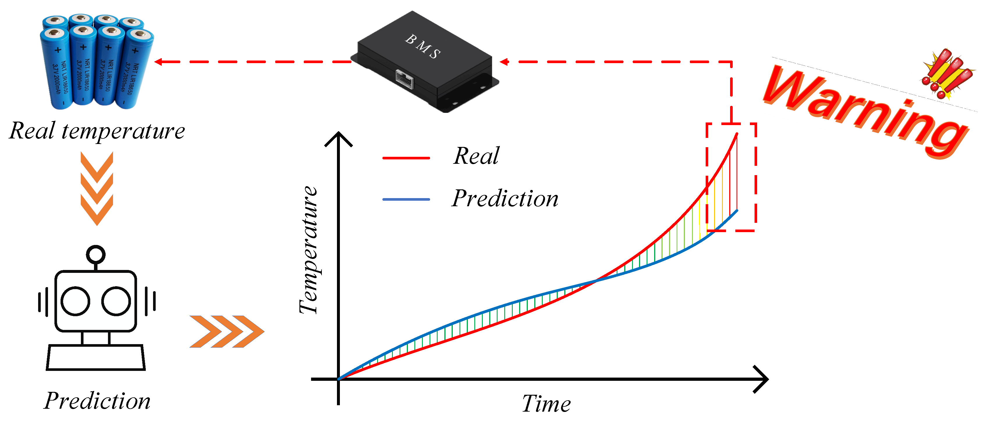
Multi-step predictions demonstrate that the performance of the EMD-Informer model, as well as the comparative models, deteriorates with an increase in prediction horizon, indicating a conflict between high predictive accuracy and a broad predictive range; the prediction horizon must be chosen appropriately to balance this conflict. Multi-step predictions show that, under the condition that the maximum absolute error is less than 0.5 °C, the hit rate for a 12-step prediction is better than that for 18-step and 24-step predictions. This achieves high predictive accuracy and a sufficiently broad prediction range, which helps in early detection of potential temperature anomalies and effectively reduces the risk of thermal runaway in the battery.

References

1. Wang, B.; Feng, Y.; Wang, S. Two-phase separation based spatiotemporal modeling of thermal processes with applications to lithium-ion batteries. Energy Storage 2022, 49, 104050. [Google Scholar] [CrossRef]
2. Cen, J.; Li, Z.; Jiang, F. Experimental Investigation on Using the Electric Vehicle Air Conditioning System for Lithium-Ion Battery Thermal Management. Energy Sustain. Dev. 2018, 45, 88–95. [Google Scholar] [CrossRef]
3. Feng, Y.; Zhou, L.; Ma, H.; Wu, Z.; Zhao, Q.; Li, H.; Zhang, K. Challenges and advances in wide-temperature rechargeable lithium batteries. Energy Environ. Sci. 2022, 15, 1711–1759. [Google Scholar] [CrossRef]
4. Zhu, S.; He, C.; Zhao, N.; Sha, J. Data-driven analysis on thermal effects and temperature changes of lithium-ion battery. J. Power Sources 2021, 482, 228983. [Google Scholar] [CrossRef]
5. Wang, Q.; Ping, P.; Zhao, X.; Chu, G.; Sun, J.; Chen, C. Thermal runaway caused fire and explosion of lithium-ion battery. J. Power Sources 2012, 208, 210–224. [Google Scholar] [CrossRef]
6. Sun, J.; Ren, S.; Shang, Y.; Zhang, X.; Liu, Y.; Wang, D. A novel fault prediction method based on convolutional neural network and long short-term memory with correlation coefficient for lithium-ion battery. J. Energy Storage 2023, 62, 106811. [Google Scholar] [CrossRef]
7. Zhu, G.; Kong, C.; Wang, J.; Kang, J.; Wang, Q.; Qian, C. A fractional-order electrochemical lithium-ion batteries model considering electrolyte polarization and aging mechanism for state of health estimation. J. Energy Storage 2023, 72, 108649. [Google Scholar] [CrossRef]
8. Miaari, A.; Ali, H. Batteries temperature prediction and thermal management using machine learning: An overview. Energy Rep. 2023, 10, 2277–2305. [Google Scholar] [CrossRef]
9. Lee, G.; Kwon, D.; Lee, C. A convolutional neural network model for SOH estimation of Li-ion batteries with physical interpretability. Mech. Syst. Signal Process. 2023, 188, 110004. [Google Scholar] [CrossRef]
10. Wu, T.; Wang, C.; Hu, Y.; Liang, Z.; Fan, C. Research on electrochemical characteristics and heat generating properties of power battery based on multi-time scales. Energy 2023, 265, 126416. [Google Scholar] [CrossRef]
11. Li, W.; Rentemeister, M.; Badeda, J.; Jost, D.; Schulte, D.; Sauer, D. Digital twin for battery systems: Cloud battery management system with online state-of-charge and state-of-health estimation. J. Energy Storage 2020, 30, 101557. [Google Scholar] [CrossRef]
12. Sun, J.; Zhu, C.; Li, L.; Li, Q. Online Temperature Estimation Method for Electric Vehicle Power Battery. CES Trans. Electr. Mach. Syst. 2017, 32, 197–203. [Google Scholar]
13. Liu, M.; Zhou, X.; Yang, L.; Ju, X. A novel Kalman-filter-based battery internal temperature estimation method based on an enhanced electro-thermal coupling model. J. Energy Storage 2023, 71, 108241. [Google Scholar] [CrossRef]
14. Qi, X.; Hong, C.; Ye, T.; Gu, L.; Wu, W. Frequency reconstruction oriented EMD-LSTM-AM based surface temperature prediction for lithium-ion battery. J. Energy Storage 2024, 84, 111001. [Google Scholar] [CrossRef]
15. Álvarez Antón, J.C.; García Nieto, P.J.; de Cos Juez, F.J.; Sánchez Lasheras, F.; González Vega, M.; Roqueñí Gutiérrez, M.N. Battery state-of-charge estimator using the SVM technique. Appl. Math. Model. 2013, 37, 6244–6253. [Google Scholar] [CrossRef]
16. Guo, Y.; Zhao, Z.; Huang, L. SoC Estimation of Lithium Battery Based on Improved BP Neural Network. Energy Procedia 2017, 105, 4153–4158. [Google Scholar] [CrossRef]
17. Li, W.; Zhu, J.; Xia, Y.; Gorji, M.B.; Wierzbicki, T. Data-driven safety envelope of lithium-ion batteries for electric vehicles. Joule 2019, 3, 2703–2715. [Google Scholar] [CrossRef]
18. Wang, Y.; Chen, X.; Li, C.; Yu, Y.; Zhou, G.; Wang, C.; Zhao, W. Temperature prediction of lithium-ion battery based on artificial neural network model. Appl. Therm. Eng. 2023, 228, 120482. [Google Scholar] [CrossRef]
19. Jiang, Y.; Yu, Y.; Huang, J.; Cai, W.; Marco, J. Li-Ion Battery Temperature Estimation Based on Recurrent Neural Networks. Sci. China Technol. Sci. 2021, 64, 1335–1344. [Google Scholar] [CrossRef]
20. Jiang, L.; Yan, C.; Zhang, X.; Zhou, B.; Cheng, T.; Zhao, J.; Gu, J. Temperature Prediction of Battery Energy Storage Plant Based on EGA-BiLSTM. Energy Rep. 2022, 8 (Suppl. S5), 1009–1018. [Google Scholar] [CrossRef]
21. Brian, B.; Chetan, K.; Matthew, D. Adaptation of an Electrochemistry-based Li-Ion Battery Model to Account for Deterioration Observed Under Randomized Use. In Proceedings of the Annual Conference of the Prognostics and Health Management Society, Fort Worth, TX, USA, 29 September–2 October 2014. [Google Scholar]
22. Liu, C.; Ge, X.; Zhang, X.; Yang, C.; Liu, Y. Research on the Characteristics of Oscillation Combustion Pulsation in Swirl Combustor. Energies 2024, 17, 4164. [Google Scholar] [CrossRef]
23. Vaswani, A.; Shazeer, N.; Parmar, N.; Uszkoreit, J.; Jones, L.; Gomez, A.; Kaiser, L.; Polosukhin, L. Attention Is All You Need. Adv. Neural Inf. Process. Syst. 2017, arXiv:1706.03762. [Google Scholar]
24. Zhou, H.; Zhang, S.; Peng, J.; Zhang, S.; Li, J.; Xiong, H.; Zhang, W. Informer: Beyond Efficient Transformer for Long Sequence Time-Series Forecasting. AAAI Conf. Artif. Intell. 2021, 35, 11106–11115. [Google Scholar] [CrossRef]
25. Rdahi, S.; AI-Majidi, S.; Abbod, M.; AI-Raweshidy, H. Machine Learning Approaches for Short-Term Photovoltaic Power Forecasting. Energies 2024, 17, 4301. [Google Scholar] [CrossRef]
Figure 1. Model-warning principle.
Energies 17 05001 g001
Figure 2. EMD algorithm processing flow.
Energies 17 05001 g002
Figure 3. The framework structure of the Informer.
Energies 17 05001 g003
Figure 4. Relevance-based reconstructed EMD-Informer model architecture.
Energies 17 05001 g004
Figure 5. Current loading probability.
Energies 17 05001 g005
Figure 6. The relationship between battery temperature and both current and voltage in dataset RW10.
Energies 17 05001 g006
Figure 7. The prediction results of the relevance-based reconstructed EMD-Informer model.
Energies 17 05001 g007
Figure 8. Prediction results and absolute errors for each model.
Energies 17 05001 g008
Figure 9. The predicted results of the test set at different stride lengths.
Energies 17 05001 g009
Figure 10. Frequency distribution of the maximum error at different stride lengths.
Energies 17 05001 g010