Research on Multi-Objective Optimization of High-Speed Solenoid Valve Drive Strategies under the Synergistic Effect of Dynamic Response and Energy Loss

Abstract

Under high-frequency operating conditions, the high-speed solenoid valve (HSV) experiences energy loss and heat generation, which significantly impacts its operational lifetime. Reducing the energy loss of an HSV without compromising its opening response characteristics poses a significant challenge. To address this issue, a finite element simulation model of an HSV coupled with a current feedback model is constructed to investigate the synergistic effects of dynamic response and energy loss. Prediction models for the opening response time, HSV driving energy, and Joule energy using a back propagation neural network (BPNN) are established. Furthermore, a multi-objective optimization study on the current driving strategy using a non-dominated sorting genetic algorithm II (NSGA-II) is conducted. After optimization, although there was a 6.24% increase in the opening response time, both HSV drive energy and Joule energy were significantly reduced by 15.67% and 22.49%, respectively. The proposed multi-objective optimization method for an HSV driving strategy holds great significance for improving its working durability.

1. Introduction

Faced with increasingly stringent emission regulations and a variety of combustion modes, the fuel injection system of diesel engines and other power machinery is required to flexibly control fuel injection strategies, such as fuel injection volume, fuel injection pressure, and fuel injection interval [1,2,3]. As the core component of the injector, the dynamic response characteristics of high-speed solenoid valves (HSVs) directly determine the fuel injection accuracy of electronically controlled injectors. Moreover, energy loss in the current drive system during its operation generates heat that affects the service life of the fuel injector [4]. Therefore, optimizing the dynamic response characteristics of the HSV opening and closing process and reducing energy losses in the current drive system are of great significance for improving the efficiency of the fuel injection systems.

Optimization studies of the HSV as the actuator of the fuel injector have been conducted from various aspects. Regarding electromagnetic materials used in HSVs, Wang et al. [5] designed a novel magnetic circuit structure based on an Al-Fe soft magnetic alloy, which effectively reduces magnetic resistance and increases magnetic conductivity, resulting in a shorter dynamic response time for HSVs. Tao et al. [6], using finite element methods, discussed the influence of soft magnetic materials and structural parameters on the magnetic circuit of the HSV while proposing an optimization design method that can achieve greater electromagnetic force and lower power consumption. Michał et al. [7], discussed how to reduce the impact of external vibrations on hydraulic valves in hydraulic drive systems. The analysis included reducing the potential vibration of the valve casing by flexibly installing the valve on the vibrating surface and also analyzed the effectiveness of materials with elastic and vibration dissipation characteristics in improving vibration isolation. This paper was significant for improving the accuracy and speed of fuel valve operation. In terms of the structure of the HSV, Liu et al. [8] proposed a novel HSV with a permanent magnet based on the parallel magnetic circuit principle, which can reduce the peak current, peak voltage, and holding current of the new HSV by 20.5%, 7.8%, and 43.9%, respectively, while increasing the response speed by 11.9% compared to the original HSV. Ebrahimi et al. [9] optimized the design of an HSV, which is composed of two opposing helical coils with a shared permanent magnet core. They considered factors such as wire length, inner diameter, average diameter, number of turns, and fill density of the coil in their optimization process. Additionally, they studied the effect of coil cross-sections with the same area but different perimeters and eccentricities on the magnetic field. The results showed that increasing eccentricity significantly enhances both the magnetic field and force at the center of the coil. In terms of a driving strategy for HSVs, Zhao et al. [10,11] found that increasing boost voltage improves opening response speed; however, this improvement diminishes as boost voltage continues to increase. They concluded that there exists an optimal boost voltage that achieves a balance between dynamic response time and effective electromagnetic energy conversion rate. Farid et al. [12] achieved a significant reduction in dynamic response time by optimizing driving parameters, such as peak current, holding current, and reverse current. Lu et al. [13] proposed a dual-power-source driving method to improve opening response times for HSVs. Their research indicated that this driving strategy can also significantly reduce the time interval between two injections.

The above studies indicate that improving the performance of the HSV can be achieved by altering its structure and driving strategy. However, as a complex electromagnetic-mechanical system, it is necessary to use multi-objective optimization methods to optimize the performance of the HSV. Li et al. [14] employed a multi-objective simulated annealing optimization algorithm to conduct multi-objective optimization designs of key structural parameters of HSVs, resulting in a 15.4% reduction in the opening response time and a 25% reduction in the closing response time. Liu et al. [15], in order to enhance the dynamic response speed of the HSV, utilized a response surface method and a genetic algorithm to determine the optimal solution where the electromagnetic force increased by 25.8% without increasing the armature mass. Li et al. [16] established a response surface model for response time based on a central composite design and conducted multi-objective optimization calculations using a genetic algorithm, resulting in a 17.7% reduction in the opening response time and a 37.4% reduction in the closing response time of the HSV. Fan et al. [17] developed a prediction model for the response time of the HSV using experimental design methods and optimized the pull-in and release response times of the HSV using a genetic algorithm, resulting in an overall response time improvement of 10.3%. Neural networks, as advanced prediction model construction algorithms, are also applicable in the multi-objective optimization of HSVs. Shen et al. [18] proposed a prediction model for the electromagnetic force based on BPNN and conducted multi-objective optimization research on the response time of the HSV in conjunction with the armature mass, achieving a reduction in the dynamic response time of the HSV. The above studies demonstrate that constructing multi-objective prediction models based on neural networks and optimizing prediction models based on genetic algorithms are feasible.

The aforementioned researchers have focused on optimizing the dynamic response characteristics of the HSV. According to Faraday’s law of electromagnetic induction, induced currents are generated inside a conductor when the magnetic field changes, forming closed loops that cause eddy currents. Therefore, during high-frequency operation, an HSV inevitably generates eddy current energy. Eddy currents can reduce the delay time between the start of the driving current decrease and the start of armature downward movement [19], but excessive eddy currents can affect the effective conversion of kinetic energy and prolong the open response time of an HSV. According to Ampere’s circuital law and Ohm’s law, passing current through a coil generates Joule heating losses. Xie et al. [20] found that a driving strategy is one of the most important factors affecting power loss and thermodynamic characteristics of HSVs, with power loss being the main heat source that raises coil temperature. At the same time, temperature rise reduces magnetic flux density and weakens the magnetic induction intensity of HSVs, increasing total energy loss significantly and affecting the durability of HSVs [21]. Therefore, considering service life, energy loss characteristics need to be taken into account when optimizing HSVs.

Currently, most research focuses more on the influence of structural and driving parameters on the dynamic response of the HSV or explores factors that affect the durability of the HSV. However, collaborative optimization for both dynamic response and energy loss is rarely carried out when optimizing the operating characteristics of HSVs. In this paper, the research object was an HSV for high-pressure common rail injectors, and prediction models for opening response time, HSV driving energy, and Joule energy based on BPNN were constructed. Considering the synergistic effect of dynamic response and energy loss, the current drive strategy of an HSV is optimized by a multi-objective genetic algorithm. The main innovation of this article is the use of the BPNN algorithm to develop a multi-objective optimization prediction model, with the driving strategy as input and dynamic response and energy loss as outputs. Additionally, the use of a genetic algorithm for multi-objective optimization is employed. The proposed multi-objective optimization method for an HSV driving strategy is of significant importance for enhancing the durability of HSV.

2. Establishment and Verification of HSV Simulation Model

2.1. Mathematical Model

The HSV consists mainly of an armature, iron core, coil, and reset spring. When driven by a periodically varying current, the HSV generates a periodically varying electromagnetic force at the core. The interaction between this electromagnetic force and the elastic force of the reset spring causes the armature to produce a reciprocating lifting motion. The HSV is a complex electromagnetic-mechanical coupling system, and the periodic current drive strategy directly affects its operating characteristics. When modeling the system, it is necessary to consider the interaction among the circuit, magnetic circuit, mechanical system, and various forms of energy generated within these systems.

In a circuit system, the coil current, voltage, resistance, and inductance relationship is as follows:

$$U=RI+N\frac{d\mathsf{\Phi }}{dt}$$

(1)

where U is the coil driving voltage, R is the coil resistance, I is the current through the coil, N is the turns number of the coil, Φ is the magnetic flux, and t is the time.

In the magnetic circuit system, the relationship between the electromagnetic force and the magnetic flux and the absorption area is as follows:

$$F_{mag}=\frac{{\mathsf{\Phi }}^2}{\mu S}$$

(2)

where F_mag is the electromagnetic force, μ is the magnetic conductivity of air, and S is the suction area.

The mechanical motion system of the HSV can be simplified as a mass–spring damper system. The motion process is described as:

$$F_{mag}-\lambda \frac{dx}{dt}-kx-F_0=m\frac{d^{2}x}{d{t}^2}$$

(3)

where λ is the damping coefficient, k is the spring stiffness, x is the armature displacement, F₀ is the spring preload force, and m is the armature mass.

In the HSV operation process, the total energy input to the circuit is the HSV drive energy E_ele., which is defined as:

$$E_{ele.}={\displaystyle {\int }_0^{t}U{I}^{}dt}$$

(4)

Various energies are also generated during the HSV operation, including eddy energy, Joule energy, elastic energy, damping energy, kinetic energy, and so on. When the driving current changes, the magnetic field changes, resulting in induced eddy currents in the iron core and forming eddy energy E_edd., which is defined as:

$$E_{edd.}={\displaystyle {\int }_0^t{\frac{C_{edd.}{f}^2{B}_m{d}^2}{\rho }}_{}dt}$$

(5)

where C_edd. is the eddy current coefficient, f is the frequency of magnetic field, B_m is the magnetic induction intensity, d is the wall thickness of the iron core, and ρ is the resistivity.

When the current passes through the coil, a certain amount of heat is generated, which is defined as the Joule energy E_Jou.:

$$E_{Jou.}={\displaystyle {\int }_0^t{I}^2{R}^{}dt}$$

(6)

The spring will be compressed when the armature moves and the elastic energy E_ela. generated is

$$E_{ela.}=\frac{1}{2}k{x}^2$$

(7)

The force of friction between the components will affect the armature movement and then generate a damping energy E_dam.. At the same time, the movement the armature will have kinetic energy E_kin..

$$E_{dam.}={\displaystyle {\int }_0^x\lambda V_d{}^{}dx}$$

(8)

$$E_{kin.}=\frac{1}{2}m{V}_d^2$$

(9)

where V_d is the moving speed of armature.

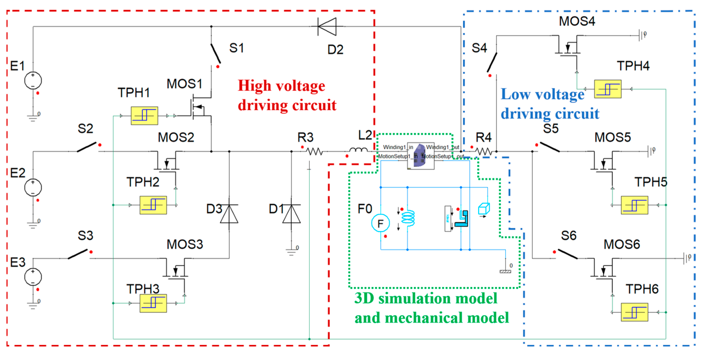
2.2. HSV Finite Element Model Coupled with Current Feedback Model

When constructing the finite element model (FEM), simplifications and assumptions regarding the geometric structure and simulation conditions of the simulated object can help improve grid quality and computational efficiency. In this study, non-magnetic components, such as gaskets and reset springs, were ignored when constructing the FEM of the HSV. Only the armature, core, and coil were modeled. Due to the symmetric structure of the HSV, only half of the model was developed. The gaps between coils were ignored and treated as an annular structure when modeling the multi-turn coil. In the simulation, elastic collisions between the armature and electromagnetic iron, as well as between the armature and valve seat, were disregarded along with any resulting deformation caused by these collisions. Based on the structure of the HSV, the maximum gap was 0.12 mm, the air gap was 0.07 mm, the number of coil turns was 52, and the preload force of the spring was 60 N. The FEM of the HSV established on the Ansoft Maxwell 19.2.0 software platform is shown in Figure 1. For the armature and core of the HSV, a mesh size of 0.5 mm was used, and for the coils, a mesh size of 1.0 mm was used. The generated mesh consisted of 86,555 elements and 15,682 nodes.

Although the Ansoft Maxwell 19.2.0 electromagnetic simulation software contains a circuit simulation module for driving the electromagnetic actuator, it cannot realize the construction of the “peak-hold-hold” current feedback driving strategy of the HSV. Therefore, this study utilized the Ansoft Maxwell 19.2.0 software and Simplorer 19.2.0 software to establish a 3D finite element model and an actual current feedback driving strategy and coupled them using Simplorer 19.2.0 to simulate the dynamic process of the HSV [22]. The calculation model for the dynamic response of the high-speed solenoid valve with current feedback is shown in Figure 2, where E1–E3 represent power supplies, S1–S6 are switches, MOS1–MOS6 are power switches, TPH1–TPH6 are hysteresis comparators, D1–D3 are diodes, L2 represents coil inductance, R3 is coil resistance, R4 is sampling resistor, and F0 denotes the preload force of spring.

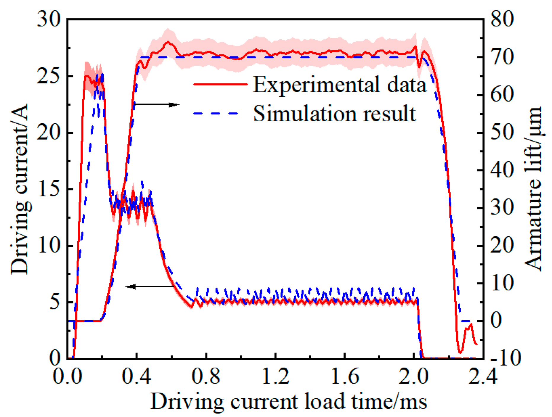
2.3. Verification of HSV Simulation Model

The accuracy of the FEM of the HSV constructed in the previous section needs to be ensured through experimental data validation. Experimental data for the HSV are obtained from a dynamic response characteristic test bench. Information regarding the setup and measurement equipment of this test bench can be found in previous studies [10,11,22]. The HSV dynamic response test bench accurately measures armature displacement within the range of 0–1 mm, while maintaining a peak voltage between 42 and 80 V and ensuring that both peak current and holding current are within limits of 25 A and 12 A, respectively.

The comparison results of the experimental data and simulated values for the armature lift and driving current curve are shown in Figure 3. In this study, the time from the start of drive current loading to when the armature reaches maximum displacement is defined as the opening stage, with its corresponding time being referred to as the opening response time. Similarly, the time from when the drive current is cut off to when the armature returns to its initial position is defined as the closing stage, with its corresponding time known as the closing response time. The interval between these two stages is referred to as the holding stage. During both the opening and closing stages of the HSV, FEM accurately predicts and captures the moments of armature pull-in and reset motion processes. In the opening stage of driving current, there is a gap between the experimental and simulated values, which is due to the influence of inductance. The inductance calibration of the HSV is based on the measurement of the electromagnetic assembly, and for the coil, its inductance value is much smaller than that of the electromagnetic assembly. In the simulation, the model uses the inductance value of the electromagnetic assembly, and a larger inductance will result in a slower change in current compared to the experimental value. However, since the inductance in the circuit is constantly changing, as the simulation progresses, the error between the current and the experimental value becomes very small. Due to collisions between the armature and iron core and valve seat during the actual operation, along with fluctuations in the drive circuit current, there may be some variation in armature lift during the holding stage. Nevertheless, the error between experimental and simulated values remains within an acceptable range during this stage. Through analysis, it can be concluded that the FEM model established in this study achieves an accurate prediction of the actual working process of the HSV while providing a solid foundation for future research.

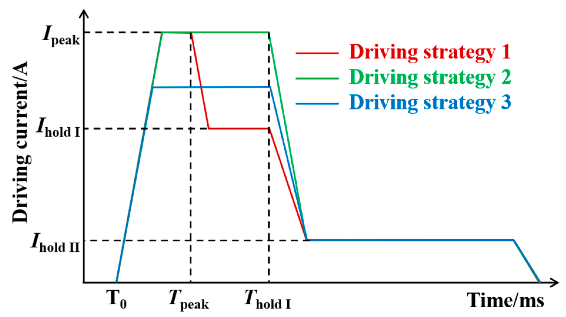
3. Influence of Driving Strategies on HSV Working Characteristics

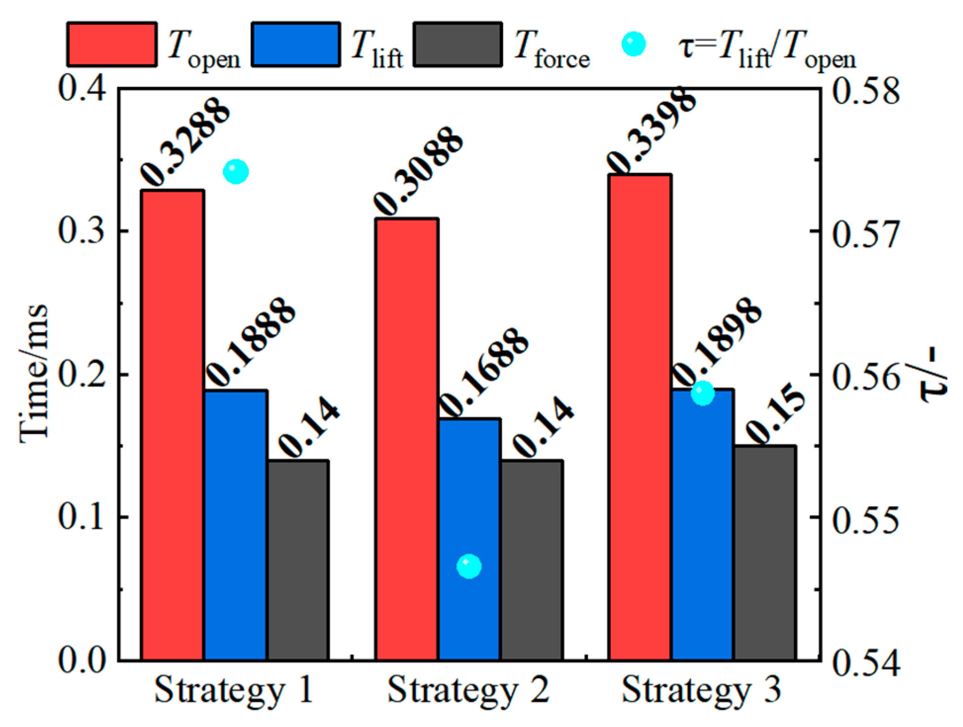
3.1. Dynamic Response Characteristics

The driving current loading strategy during the opening stage not only affects the response time of the HSV but also significantly impacts energy loss. This study analyzes the driving strategy at the moment of HSV opening, investigating the effects of different strategies on dynamic response and energy consumption characteristics during this stage. The original driving strategy for the HSV is a “peak-hold-hold” type. To optimize it, this study proposes two modified strategies based on the original. Figure 4 illustrates the timing of current loading for both the original “peak-hold-hold” strategy and two “peak-hold” strategies. Driving Strategy 1 represents the original approach, while in Driving Strategy 2 the peak current loading time is equal to that of the Driving Strategy 1 plus a first-order hold current loading time. In Driving Strategy 3, the peak current falls between Strategies 1 and 2, with a consistent peak current loading time as in Strategy 2. Specific parameters for each driving strategy are shown in

Table 1. Parameter comparison of different driving strategies.

Design Variable, Symbol	Unit	Strategy 1	Strategy 2	Strategy 3
Peak voltage, Vpeak	V	70	70	70
Peak current, Ipeak	A	24.5	24.5	19
Peak current loading time, Tpeak	s	0.00023	0.00049	0.00049
First-order holding current, Ihold I	A	14	-	-
First-order holding current loading time, Thold I	s	0.00049	-	-
Second-order holding current, Ihold II	A	5	5	5

.

The comparison of the armature lift and electromagnetic force curves of the HSV under different driving strategies is shown in Figure 5. During the opening stage, the armature rising time of the HSV is the same for all three driving strategies, while Driving Strategy 2 has the shortest time for the armature to reach maximum displacement, and Driving Strategy 3 has the longest time. Additionally, in the early stage of motion, there is an overlap between lift curves for Driving Strategies 1 and 2. This occurs because, in Driving Strategy 1, the armature has not yet reached maximum displacement when the driving current begins to decrease to 14 A, entering into a first-order holding stage. Within a certain range, a larger peak current and first-order holding current result in a shorter opening response time for the HSV. From observing changes in trends within electromagnetic force curves, it can be seen that the electromagnetic force starts generating when the current begins loading and reaches its peak when the armature moves near maximum displacement before starting to decrease. At 0.49 ms, the current enters the final holding stage where the electromagnetic force decreases to 110 N. The magnitude of the electromagnetic force strongly correlates positively with the current within the circuit. Therefore, increasing the current during the opening stage can be considered to minimize the opening time. Considering the pre-loading force of the spring at 60 N allows room for current decrease during the holding stage. However, any changes made to the driving strategy need to consider the variation in energy consumption.

From the figure above, it can be observed that the moment when the displacement of the armature begins to change during the opening stage is inconsistent with the time when the electromagnetic force increases. The armature only starts to move when the electromagnetic force reaches approximately 110 N. Therefore, to thoroughly evaluate the impact of different driving strategies on the opening stage of the HSV, the ratio of the armature motion time (T_lift) to the solenoid valve opening response time (T_open) is defined as the effective time ratio (τ). The overcoming resistance time (T_force) of the HSV is then calculated as the difference between the HSV opening response time and the armature motion time, T_force = T_open − T_lift. Figure 6 illustrates the effects of different driving strategies on T_open, T_lift, T_force, and τ. A comparison between Driving Strategies 1 and 2 reveals that their T_force values are consistent, both at 0.14 ms, while the T_lift of Driving Strategy 2 is shorter than that of Driving Strategy 1, indicating that increasing the first-order holding current can reduce T_lift in the peak-hold-hold driving strategy. Contrasting Driving Strategies 1 and 3, it is found that the deviation of T_lift is only 0.53%, while the deviation of T_open is 3.35%. Consequently, the peak current significantly affects T_force in the peak-hold-hold driving strategy. In terms of τ, Driving Strategy 1 is the largest, followed by Driving Strategy 3, and Driving Strategy 2 is the smallest, indicating that Driving Strategy 1 can effectively convert kinetic energy for armature motion.

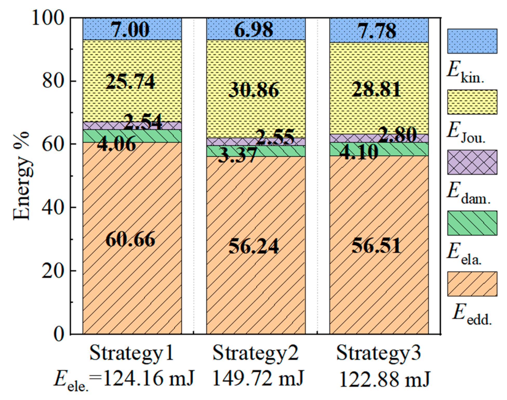
3.2. Energy Consumption Characteristics

The larger the driving current during the opening stage, the shorter the response time of the HSV. However, a larger driving current also leads to greater energy loss. Therefore, when optimizing driving strategies, it is necessary to consider the synergistic effect of dynamic response and energy loss. Figure 7 illustrates the energy loss during the opening stage under different driving strategies. Across various driving strategies, eddy current energy and Joule energy during the opening stage account for more than 85% of the total energy, with eddy current energy representing over 55% of the total energy. Due to the longest peak current loading time in Strategy 2, the HSV has the highest total energy consumption at 149.72 mJ compared to Strategies 1 and 3 which have relatively similar total energies. Since the rate of change in the current increases, so does the eddy current energy. Similarly, as the current increases, so does the Joule energy. Consequently, during the opening stage, Driving Strategy 1 has a higher proportion of eddy current energy and a lower proportion of Joule energy compared to Driving Strategies 2 and 3 which have similar proportions of eddy current energy but with Driving Strategy 2 having a higher proportion of Joule energy. However, in terms of specific energy loss, the eddy current energy and Joule energy of Drive Strategy 2 are the largest, 84.20 mJ and 46.20 mJ, respectively. The eddy current energy of Drive Strategy 3 and the Joule energy of Drive Strategy 1 are the smallest, 69.07 mJ and 31.96 mJ, respectively.

The trend of eddy current energy and Joule energy, which account for the largest proportion of energy loss, over the entire HSV working cycle is illustrated in Figure 8. Regarding Joule energy, its trend follows that of the drive current. When the driving current fluctuates at approximately 24.5 A, 230 W of Joule energy will be generated. When the drive current fluctuates at approximately 19 A, 138 W of Joule energy will be generated, and when the drive current is at 14 A, the Joule energy is 75 W. Combined with Equation (6), it can be observed that the Joule energy is proportional to the square of the current, and thus, a greater peak current leads to a greater Joule energy loss. As for eddy current energy, its value increases with a higher rate of change in current. Therefore, during stages of peak current loading, there is a significant instantaneous change in current resulting in a large amount of eddy current energy loss inside both armature and core components of the HSV. Under different driving strategies and as the currents enter into the holding stage, there will be a significant reduction in eddy current energy inside the HSV.

Combined with the previous analysis of the dynamic response characteristics of the HSV, it can be concluded that in the peak-hold-hold driving strategy, increasing the peak current can shorten the time required to overcome resistance for the HSV. However, this will significantly increase the Joule energy loss. On the other hand, increasing the first-order holding current can reduce armature motion time, and rapidly changing current can increase eddy current energy.

4. Optimization of HSV Driving Strategy Based on BPNN-NSGA-II

The trade-off relationship between energy loss and opening response time requires decision-making based on specific requirements when optimizing driving strategies. This study utilized multiple parameters within the peak-hold-hold driving strategy of an HSV on a diesel engine as variables, with Joule energy, HSV driving energy, and opening response time as targets for optimization. The BPNN was employed to construct prediction models for optimizing objectives while NSGA-II was used for multi-objective optimization analysis. Figure 9 illustrates the multi-objective optimization process coupled with BPNN and NSGA-II.

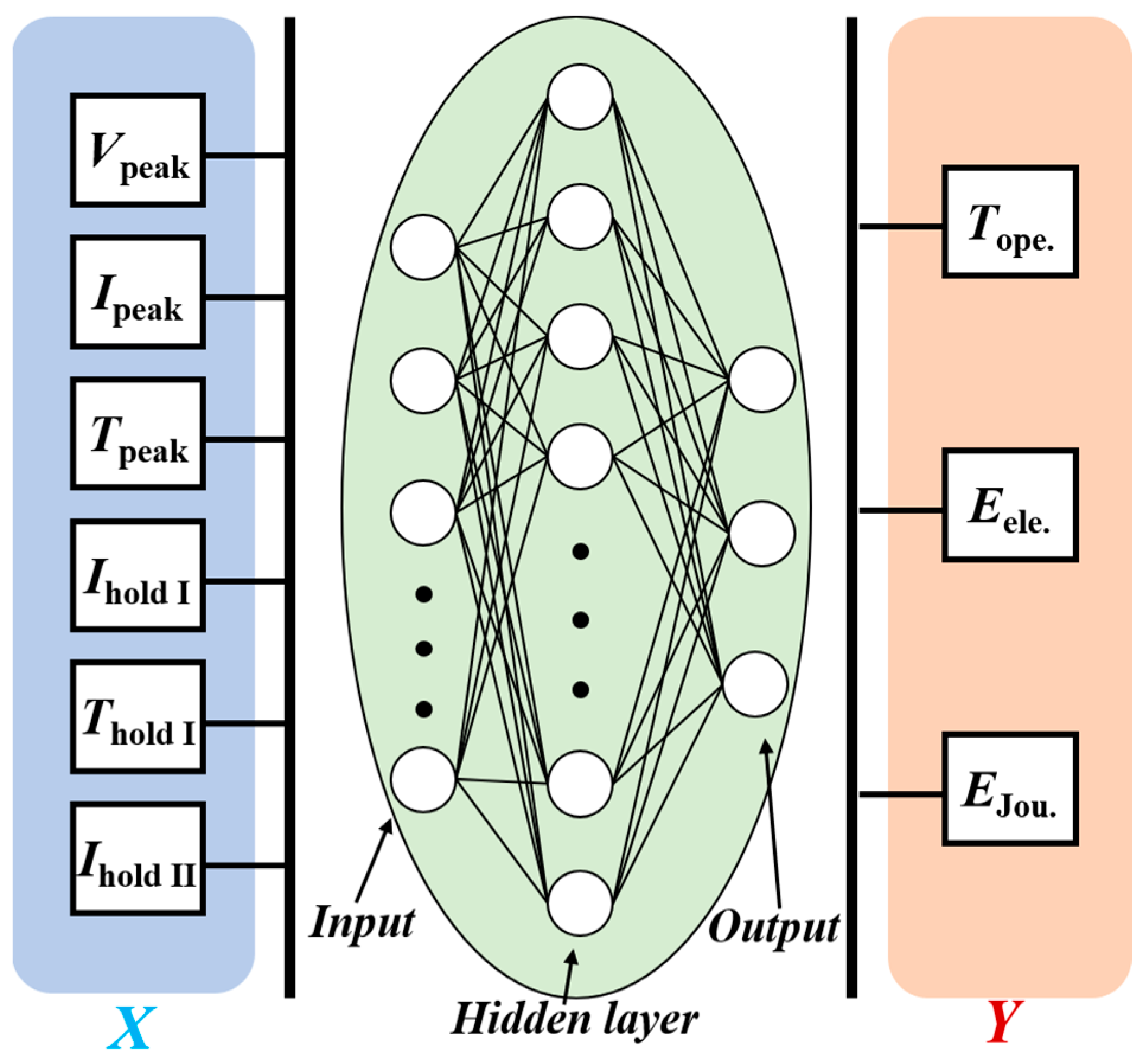
4.1. Prediction Model of BPNN

4.1.1. Sample Data

In this study, six parameters in the driving strategies were selected for a high-pressure common rail injector HSV, including peak voltage, peak current, peak current loading time, first-order holding current, first-order holding current loading time, and second-order holding current. The geometric structural parameters remained unchanged.

Table 2. The parameter variation ranges.

Design Variable	Level
	Lower		Standard		Upper
Vpeak/V	65	67.5	70	72.5	75
Ipeak/A	23	23.75	24.5	25.25	26
Tpeak/s	0.00021	0.00022	0.00023	0.00024	0.00025
Ihold I/A	12	13	14	15	16
Thold I/s	0.00045	0.00047	0.00049	0.00051	0.00053
Ihold II/A	4	4.5	5	5.5	6

presents the variation in the six-factor five-level parameters for the HSV driving parameters. In the table, the baseline values represent the original driving parameters of the HSV sample. The selection range for each parameter is based on the standard value, with an equal increase or decrease as the upper and lower limits of the parameter change. When selecting these limits, it was essential to ensure that all combinations of parameter changes can work normally for HSVs. The experimental design method chosen was a D-optimal design method which statistically studies different experimental designs and establishes an optimal approach. Therefore, regression values obtained based on this method exhibit a high degree of fit with observed values and hold statistical significance [23,24,25].

Using the D-optimal design method resulted in obtaining 94 sets of sample data for developing a prediction model while randomly selecting 19 sets as testing sets for BPNN; the remaining 75 sets were utilized as training sets. All sample points in both training and testing sets were obtained through FEM simulation calculations constructed in the previous section.

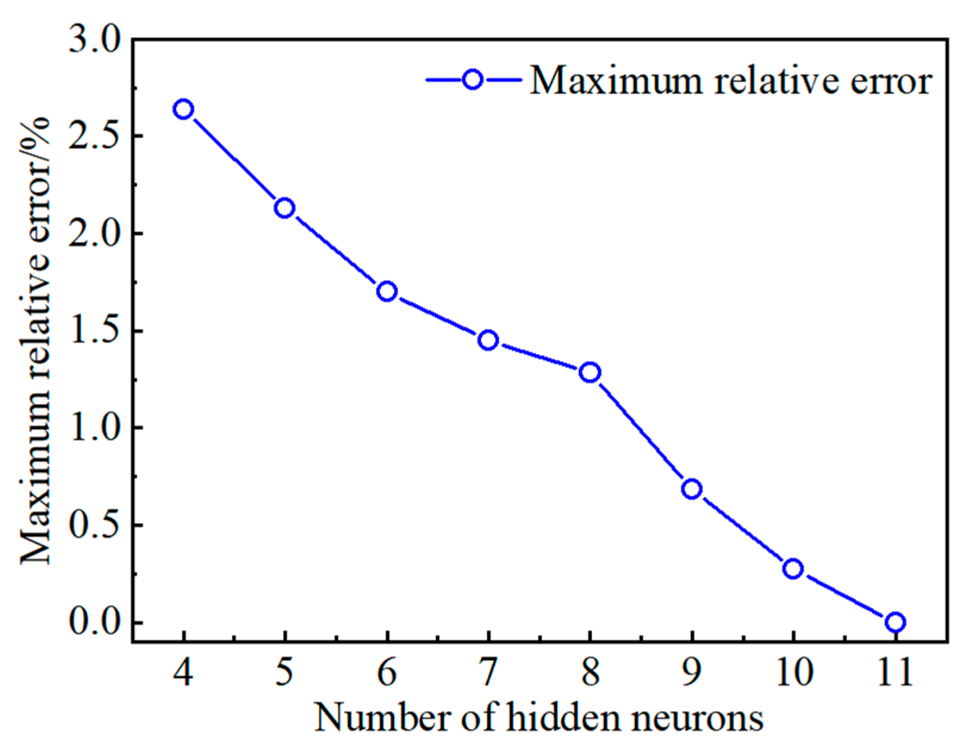
4.1.2. Model Training

A typical n-dimensional input neuron model consists of inputs, network weights and thresholds, summation units, transfer functions, and outputs [26,27]. The n input variables of the neuron can be represented as a column vector X:

$$X={[x_1,x_2,\cdots ,x_n]}^T$$

(10)

The weight of the network connects the input variables with the neuron and can be represented as a vector W:

$$W=[w_{11},w_{12},\cdots ,w_{1n}]$$

(11)

The threshold of the network is a scalar, denoted as b. The performance of network can be adjusted through the weights and thresholds.

The summation unit is the first process for processing the input signals in the neural network and is used to weight the input signals:

$$net={\displaystyle \sum _{k=1}^n{x}_k{w}_{1k}+b}$$

(12)

The function operation on the weighted signal is the second process for processing the input signal in the neural network, and the most commonly used function is the Sigmoid function:

$$f(x)=\frac{1}{1+e^{-x}}$$

(13)

After weighted summation and function operation of the input signal, the final output is

$$y=f(wx+b)$$

(14)

A typical BPNN model consists of an input layer, a hidden layer, and an output layer. During the training process of the prediction model, the neurons in each layer are only influenced by the neurons in the previous layer. When the signal propagates from the input layer to the hidden layer and then to the output layer without reaching the expected threshold, it will be propagated back from the output layer to the input layer. After adjusting the network weights of each layer, this signal propagation is repeated. After multiple forward and backward signal transmissions, finally, the expected signal can be obtained. The structure of BPNN is uncertain, and selecting a reasonable number of network layers and neurons is a prerequisite for achieving optimal performance.

For this study, the number of neurons in the input layer corresponds to the number of driving parameters, while the number of neurons in the output layer corresponds to the number of optimization objectives. In other words, there are six neurons in the input layer and three neurons in the output layer. The accuracy of the prediction model is affected by both the number and size of the hidden layers. Generally speaking, a single hidden layer is preferred for constructing BPNNs. If a single hidden layer fails to produce accurate results, double or multiple hidden layers can be used instead [28,29]. Based on preliminary research findings that indicate satisfactory accuracy levels with a single hidden layer structure network, this study has chosen to use such a structure for BPNN as shown in Figure 10.

The number of hidden layers has been determined, and it is necessary to further determine the number of neurons in the hidden layer. In this study, the method of repeated experiments was used to compare the relative errors of models with different numbers of neurons, as shown in Figure 11. As the number of neurons within the hidden layer increases, the relative error of the prediction model for the Joule energy gradually decreases. When there are more than eight neurons, the relative error is less than 1%. However, when there are 11 neurons, overfitting occurs with a relative error of 1.57 × 10⁻¹⁰%. Therefore, through comparison, it is concluded that there should be 10 neurons in the hidden layer of the BPNN in this study, where the relative error for predicting the Joule energy is 0.27%.

4.1.3. Model Verification

The prediction models for the opening response time, HSV driving energy, and Joule energy have been obtained through repeated training and validation. Figure 12 shows the comparison between the prediction values obtained from the BPNN-trained model and the simulation results obtained from FEM, where Equation (15) is used to calculate the R² values of each model. The R² values of the prediction models for the opening response time, HSV driving energy, and Joule energy are 0.972, 0.988, and 0.991, respectively. Therefore, the BPNN-trained prediction model demonstrates good prediction accuracy and generalization ability, making it suitable for subsequent multi-objective optimization analysis.

$$R^2=1-\frac{{\displaystyle \sum _{i=1}^n{(y_i-f(x_i))}^2}}{{\displaystyle \sum _{i=1}^n{(y_i-\overline{y})}^2}}$$

(15)

4.2. Multi-Objective Optimization Model of NSGA-II

The genetic algorithm simulates the process of natural selection to solve problems and select results. It has great potential in solving complex optimization problems and is widely used in automatic control, transportation, and other fields [30,31]. For multi-objective optimization problems, Srinivas et al. [32] proposed the NSGA algorithm based on the non-dominated sorting principle. Deb et al. [33] further introduced the elite strategy, crowding distance, and crowding comparison operators and proposed the NSGA-II algorithm. In this study, a multi-objective optimization mathematical model was constructed based on the prediction model trained by BPNN, and the NSGA-II algorithm was used for optimization research.

The multi-objective optimization mathematical model comprises variables, objectives, and constraints. The following definitions and constraints are formulated for the three-objective optimization problem in this study:

$$X={[x_1,x_2,\cdots ,x_6]}^T={[V_{peak},I_{peak},T_{peak},I_{hold}{}_I,T_{hold}{}_I,I_{hold}{{}_{}}_{II}]}^T$$

(16)

$$MinF\left(X\right)={[f_1\left(x^{\prime }\right),f_2\left(x^{\prime }\right),f_3\left(x^{\prime }\right)]}^T={[T_{\mathrm{ope}.},E_{\mathrm{ele}.},E_{\mathrm{Jou}.}]}^T$$

(17)

$$s.t.\{\begin{array}{l}Minimum\le X\le Maximum;\\ f\left(x^{\prime }\right)\le f\left(x\right);\end{array}$$

(18)

where x_i (i = 1, 2, ⋯, 6) is the initial value of the variable, $x_i^{\prime }$ (i = 1, 2, ⋯, 6) is the optimized value of the variable, and f(x) is the BPNN prediction model.

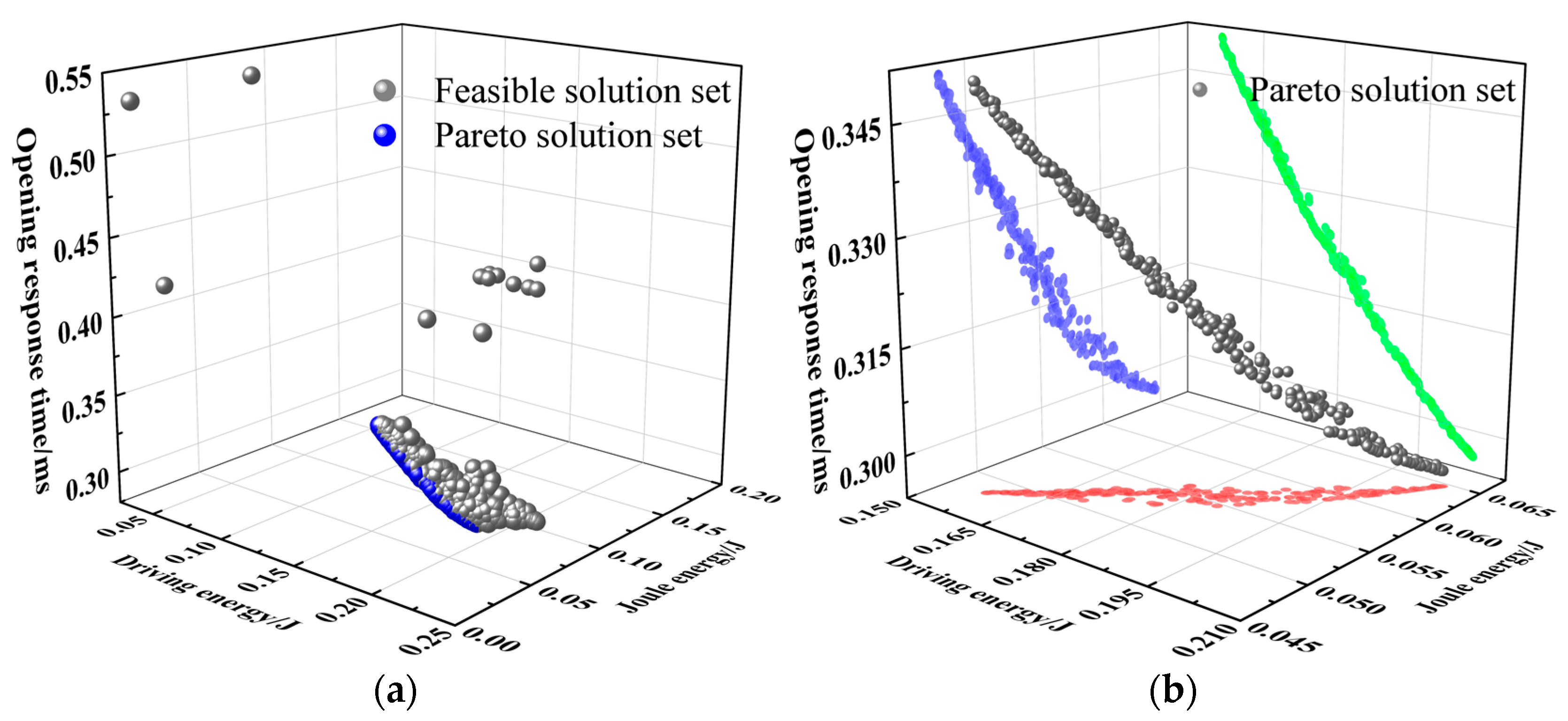
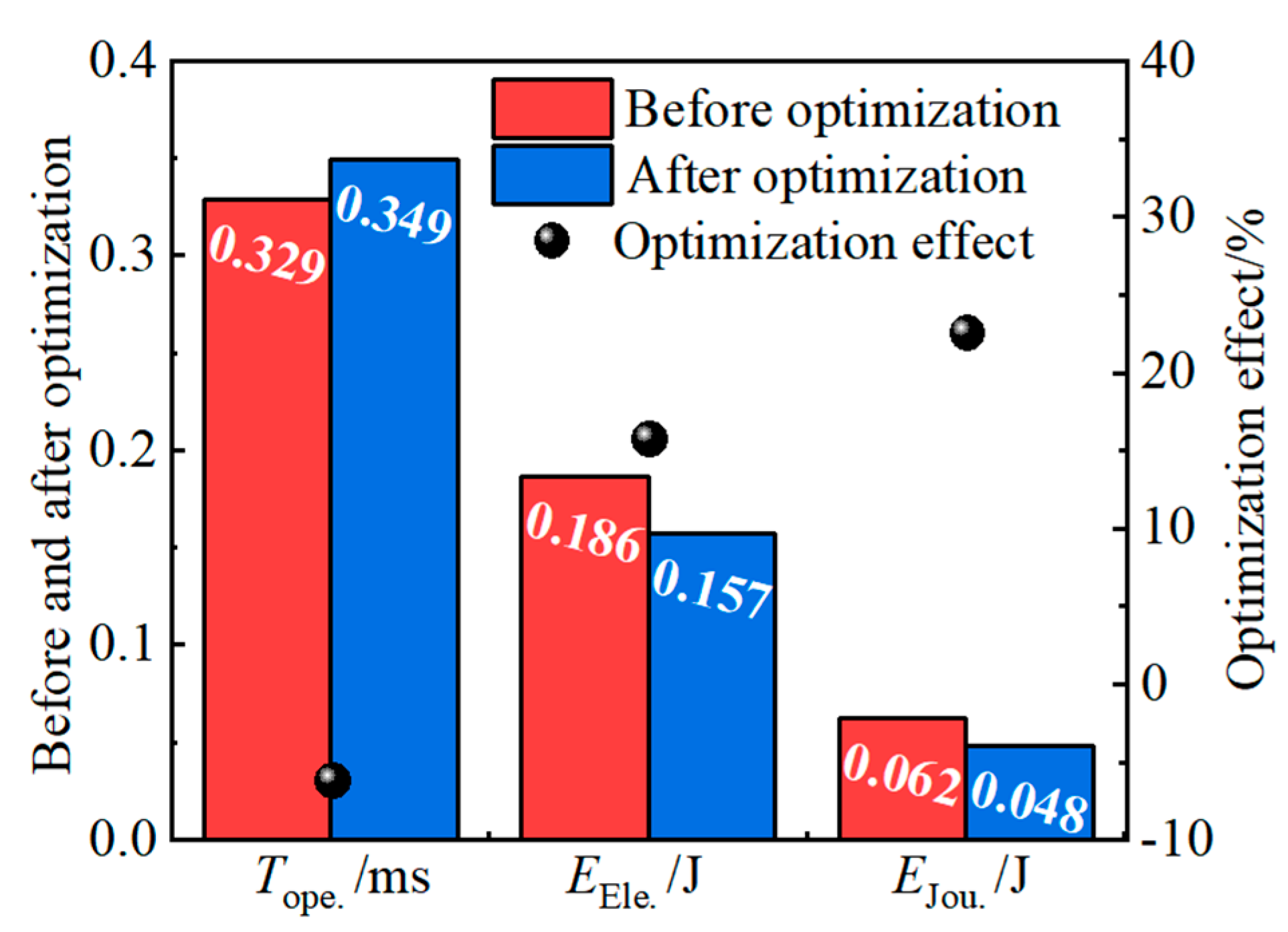
4.3. Optimization Results

The termination iteration in the genetic algorithm was set to 2000, with a crossover rate of 0.9 and a mutation rate of 0.5. After iterative calculations based on the multi-objective optimization model, Figure 13a shows the distribution of all feasible solutions that satisfy the constraints, while Figure 13b shows the distribution of the Pareto solution set. The Pareto solution set refers to a group of solutions where no solution can be improved in terms of one objective function without sacrificing the values of other objective functions. For a two-objective optimization problem, the Pareto solution set forms a curve; while for three or more objectives, it forms a surface or hypersurface. From Figure 13a, it can be observed that the majority of feasible solutions are concentrated together, with only a few distributed on the periphery, indicating that the genetic algorithm iterated near the optimal solution within a limited number of iterations. As for the Pareto solution set shown in Figure 13b, they are distributed outside the feasible solutions and form an irregular surface. The blue, red, and green symbols represent the projections of the Pareto solution set on different coordinate plane. This indicates an inverse relationship between T_ope. and E_ele., meaning that as HSV driving energy decreases and opening response time increases. Additionally, there is a positive correlation between E_ele. and E_Jou., where an increase in driving energy leads to a larger Joule energy. There exists a trade-off relationship between T_ope., E_ele., and E_Jou., and there is no optimal solution that simultaneously minimizes T_ope., E_ele., and E_Jou..

In this study, the minimum distance method [34] was used to filter the Pareto solution set in order to obtain the optimal solution that achieves the best overall performance of the HSV. Considering the different units of T_ope., E_ele., and E_Jou., implementing the minimum distance method requires defining dimensionless objective functions, calculating the minimum distance, and selecting the point with the minimum distance. The dimensionless definition of an objective function is given by Equations (19)–(22). By comparing the Pareto solutions with their corresponding objective values before optimization, the influence of different units on decision-making is eliminated.

$$T_{ope.}{}^{*}=\frac{T_{ope.}{}^{\prime }}{T_{ope.}}$$

(19)

$$E_{ele.}{}^{*}=\frac{E_{ele.}{}^{\prime }}{E_{ele.}}$$

(20)

$$E_{Jou.}{}^{*}=\frac{E_{Jou.}{}^{\prime }}{E_{Jou.}}$$

(21)

$$\min D=\sqrt{{\left(T_{ope.}{}^{*}\right)}^2+{\left(E_{ele.}{}^{*}\right)}^2+{\left(E_{Jou.}{}^{*}\right)}^2}$$

(22)

where T_ope. and $T_{ope.}{}^{\prime }$ represent the pre-optimized and post-optimized opening response time, and $T_{ope.}{}^{*}$ represents the dimensionless opening response time. The same applies to the E_ele., and E_Jou..

Figure 14 shows the comparison of the opening response time, HSV driving energy, and Joule energy of the HSV before and after optimization. After optimization, the opening response time increased by 6.24% from 0.329 ms to 0.349 ms. However, both the HSV driving energy and Joule energy decreased to different extents. The HSV driving energy was reduced by 15.67% from 0.186 J to 0.157 J, while the Joule energy decreased by 22.49% from 0.062 J to 0.048 J. The optimization results indicate that using the minimum distance method for filtering the Pareto solution set resulted in a little bit longer opening response time for the HSV, reduced energy consumption, and decreased Joule heat generation. Since Joule heat directly affects the working life of the HSV, the optimized HSV can reduce energy by 38%, thus significantly enhancing the working life of the HSV.

Table 3. Comparison of optimization parameters before and after optimization.

Design Variable	Before Optimization	After Optimization
Vpeak/V	70	65
Ipeak/A	24.5	23.0
Tpeak/s	0.00023	0.00021
Ihold I/A	14	12
Thold I/s	0.00049	0.000457
Ihold II/A	5	4

shows the comparison of optimization parameters before and after optimization. After optimization, the current and voltage are reduced to different degrees.

5. Conclusions

This study focuses on the HSV of a diesel injector, considering the synergistic effects of dynamic response and energy loss. It conducts a multi-objective optimization study on the driving strategy of the HSV and draws the following conclusions:

(1) An FEM of the HSV coupled with a current feedback model was constructed. The analysis, based on the validated model, investigated the impacts of different driving strategies on the dynamic response characteristics and energy loss of the HSV. The peak current significantly affects the time for the HSV to overcome resistance, while increasing the first-order holding current can shorten armature movement time. Eddy current energy and Joule energy account for over 85% of the total energy. The eddy current energy and Joule energy of Drive Strategy 2 are the largest, 84.20 mJ and 46.20 mJ, respectively. The eddy current energy of Drive Strategy 3 and the Joule energy of Drive Strategy 1 are the smallest, 69.07 mJ and 31.96 mJ, respectively. Lower energy loss can reduce Joule heat generation, thus improving the working life of the HSV.

(2) A set of 94 sample points was generated based on the D-optimal design method, and a study was conducted in order to develop prediction models for the opening response time, HSV driving energy, and Joule energy by utilizing BPNN. The R² values of the prediction models were 0.972, 0.988, and 0.991, respectively. A multi-objective optimization model was established based on these prediction models, and NSGA-II was used for the optimization analysis resulting in a Pareto solution set for the three optimization objectives. There is a trade-off relationship between the opening response time, HSV driving energy, and Joule energy.

(3) The Pareto solution set was filtered using the minimum distance method to obtain the final optimization results. After optimization, the drive voltage is reduced by 5 V, and the peak current, first-order current, and second-order current are reduced by 1.5 A, 2 A and 1 A, respectively. And the opening response time was extended from 0.329 ms to 0.349 ms, HSV driving energy decreased from 0.186 J to 0.157 J, and Joule energy decreased from 0.062 J to 0.048 J. The optimization effects were −6.24%, 15.67%, and 22.49%, respectively. The optimized HSV significantly reduced energy consumption and generation of Joule energy while only slightly extending the dynamic response time.

The multi-objective optimization method based on BPNN-NSGA-II proposed in this paper demonstrates good capability for optimizing HSV and addressing energy loss issues, thereby enhancing its working lifetime. In the next stage, the design and testing of HSV samples will be carried out based on the multi-objective optimization results to further evaluate the effectiveness of the optimizations.

References

1. Duan, X.; Lai, M.C.; Jansons, M.; Guo, G.; Liu, J. A review of controlling strategies of the ignition timing and combustion phase in homogeneous charge compression ignition (HCCI) engine. Fuel 2021, 285, 119142. [Google Scholar] [CrossRef]
2. Shi, Z.; Lee, C.-F.; Wu, H.; Li, H.; Wu, Y.; Zhang, L.; Bo, Y.; Liu, F. Effect of injection pressure on the impinging spray and ignition characteristics of the heavy-duty diesel engine under low-temperature conditions. Appl. Energy 2020, 262, 114552. [Google Scholar] [CrossRef]
3. Shi, Z.; Wu, H.; Li, H.; Zhang, L.; Li, X.; Lee, C.-F. Effect of injection pressure and fuel mass on wall-impinging ignition and combustion characteristics of heavy-duty diesel engine at low temperatures. Fuel 2021, 299, 120904. [Google Scholar] [CrossRef]
4. Ishii, E.; Yoshimura, K.; Yasukawa, Y.; Ehara, H. Effects of Opening and Closing Fuel-Injector Valve on Air/Fuel Mixture. J. Eng. Gas Turbines Power 2017, 139, 092804. [Google Scholar] [CrossRef]
5. Wang, Q.; Yang, F.; Yang, Q.; Chen, J.; Guan, H. Experimental analysis of new high-speed powerful digital solenoid valves. Energy Convers. Manag. 2011, 52, 2309–2313. [Google Scholar] [CrossRef]
6. Tao, G.; Chen, H.Y.; YY, J.; He, Z.B. Optimal design of the magnetic field of a high-speed response solenoid valve. J. Mater. Process. Technol. 2002, 129, 555–558. [Google Scholar] [CrossRef]
7. Stosiak, M.; Karpenko, M.; Prentkovskis, O.; Deptuła, A.; Skačkauskas, P. Research of vibrations effect on hydraulic valves in military vehicles. Def. Technol. 2023, 30, 111–125. [Google Scholar] [CrossRef]
8. Liu, P.; Fan, L.; Zhou, W.; Ma, X.; Song, E. Dynamic performances analysis and optimization of novel high-speed electromagnetic actuator for electronic fuel injection system of diesel engine. J. Mech. Sci. Technol. 2017, 31, 4019–4028. [Google Scholar] [CrossRef]
9. Ebrahimi, N.; Schimpf, P.; Jafari, A. Design optimization of a solenoid-based electromagnetic soft actuator with permanent magnet core. Sens. Actuators A Phys. 2018, 284, 276–285. [Google Scholar] [CrossRef]
10. Zhao, J.; Wang, M.; Wang, Z.; Grekhov, L.; Qiu, T.; Ma, X. Different boost voltage effects on the dynamic response and energy losses of high-speed solenoid valves. Appl. Therm. Eng. 2017, 123, 1494–1503. [Google Scholar] [CrossRef]
11. Zhao, J.; Yue, P.; Grekhov, L.; Ma, X. Hold current effects on the power losses of high-speed solenoid valve for common-rail injector. Appl. Therm. Eng. 2018, 128, 1579–1587. [Google Scholar] [CrossRef]
12. Breidi, F.; Helmus, T.; Lumkes, J. The impact of peak-and-hold and reverse current solenoid driving strategies on the dynamic performance of commercial cartridge valves in a digital pump/motor. Int. J. Fluid Power 2016, 17, 37–47. [Google Scholar] [CrossRef]
13. Lu, H.; Deng, J.; Hu, Z.; Wu, Z.; Li, L. Impact of Control Methods on Dynamic Characteristic of High Speed Solenoid Injectors. SAE Int. J. Engines 2014, 7, 1155–1164. [Google Scholar] [CrossRef]
14. Li, T.; Zhang, Y.; Wang, D.; Xiong, Q. Optimization Design of High-speed Solenoid Based on Multi-objective Simulated Annealing Method. Veh. Engine 2010, 4, 6–10. (In Chinese) [Google Scholar]
15. Liu, P.; Fan, L.; Xu, D.; Ma, X.; Song, E. Multi-Objective Optimization of High-Speed Solenoid Valve Based on Response Surface and Genetic Algorithm; SAE Technical Paper 2015, 2015-01-1350; Harbin Engineering University: Harbin, China, 2015. [Google Scholar]
16. Li, T.; Zhang, Y.; Liang, Y.; Yang, Y.; Jiao, J. Multiobjective optimization research on the response time of a pneumatic pilot-operated high speed on/off valve. Int. J. Appl. Electromagn. Mech. 2021, 65, 109–127. [Google Scholar] [CrossRef]
17. Fan, L.; Zhou, W.; Liu, P.; Zhao, J.; Grekhov, L. Multiobjective optimization of dynamic response of high speed solenoid valve. J. Harbin Eng. Univ. 2018, 39, 53–59. (In Chinese) [Google Scholar]
18. Shen, D.; Hao, Z.; Zhao, G.; Li, X. Multi-objective optimization design of solenoid valve based on BP neural network. J. Xi’an Polytech. Univ. 2023, 37, 1–8. (In Chinese) [Google Scholar]
19. Li, M.; Zhang, Y. Influence of eddy current on transient characteristics of common rail injector solenoid valve. J. Beijing Inst. Technol. 2015, 24, 26–34. [Google Scholar]
20. Xie, N.; Zhang, Z.; Yin, C. Power losses and thermodynamic analysis of the solenoid fuel injector. Int. J. Appl. Electromagn. Mech. 2017, 54, 405–419. [Google Scholar] [CrossRef]
21. Cheng, Q.; Xu, M.; Zhang, Z.; Xie, N. FEM simulation and performance analysis of a novel heated tip SIDI injector. Int. J. Heat Fluid Flow 2016, 59, 87–99. [Google Scholar] [CrossRef]
22. Zhao, J.; Zirka, S.E.; Moroz, Y.I. Duality-Derived Models of High-Speed Electromagnetic Valves. IEEE Trans. Ind. Electron. 2021, 68, 9876. [Google Scholar] [CrossRef]
23. Eriksson, L.; Johansson, E.; Kettaneh-Wold, N.; Wikström, C.; Wold, S. Design of experiments. In Principles and Applications, 3rd ed.; Umetrics Academy: Umea, Sweden, 2008. [Google Scholar]
24. Myers, R.H.; Montgomery, D.C.; Anderson-Cook, C.M. Response Surface Methodology: Process and Product Optimization Using Designed Experiments, 3rd ed.; John Wiley and Sons: Hoboken, NJ, USA, 2009. [Google Scholar]
25. Kuram, E.; Ozcelik, B.; Bayramoglu, M.; Demirbas, E.; Simsek, B.T. Optimization of cutting fluids and cutting parameters during end milling by using D-optimal design of experiments. J. Clean. Prod. 2013, 42, 159–166. [Google Scholar] [CrossRef]
26. Lecun, Y.; Bengio, Y.; Hinton, G. Deep Learning. Nature 2015, 521, 436–444. [Google Scholar] [CrossRef] [PubMed]
27. Wang, G.; Awad, O.I.; Liu, S.; Shuai, S.; Wang, Z. NOx emissions prediction based on mutual information and back propagation neural network using correlation quantitative analysis. Energy 2020, 198, 117286. [Google Scholar] [CrossRef]
28. Ma, X.; Liu, D. Comparative Study of Hybrid Models Based on a Series of Optimization Algorithms and Their Application in Energy System Forecasting. Energies 2016, 9, 640. [Google Scholar] [CrossRef]
29. Dong, Y.; Ma, X.; Ma, C.; Wang, J. Research and Application of a Hybrid Forecasting Model Based on Data Decomposition for Electrical Load Forecasting. Energies 2016, 9, 1050. [Google Scholar] [CrossRef]
30. Yu, Z.; Wei, S.; Wu, C.; Wu, L.; Sun, L.; Zhang, Z. Development and verification of RP-3 aviation kerosene surrogate fuel models using a genetic algorithm. Fuel 2022, 312, 122853. [Google Scholar] [CrossRef]
31. Marler, R.T.; Arora, J.S. Survey of multi-objective optimization methods for engineering. Struct. Multidiscip. Optim. 2004, 26, 369–395. [Google Scholar] [CrossRef]
32. Srinivas, N.; Deb, K. Multi-objective function optimization using nondominated sorting genetic algorithms. Evol. Comput. 1995, 2, 221–248. [Google Scholar] [CrossRef]
33. Deb, K.; Agrawal, S.; Pratap, A.; Meyarivan, T. A fast elitist nondominated sorting genetic algorithm for multi-objective optimization: NSGA-II. In Proceedings of the International Conference on Parallel Problem Solving from Nature, Paris, France, 18–20 September 2000; pp. 849–858. [Google Scholar]
34. Gu, Y.; Fan, L.; Lan, Q.; Wei, Y.; Zhou, J.; Du, K. Multi-objective optimization of fuel injection performance of a common rail injector. Int. J. Engine Res. 2023, 24, 3282–3296. [Google Scholar] [CrossRef]
Figure 1. The simplified 3D simulation model of HSV.
Energies 17 00300 g001
Figure 2. Dynamic response simulation model of HSV with current feedback.
Energies 17 00300 g002
Figure 3. Comparison of simulation results and experimental data of HSV FEM.
Energies 17 00300 g003
Figure 4. Schematic diagram of current loading timing for different driving strategies.
Energies 17 00300 g004
Figure 5. Comparison of armature lift and electromagnetic force curves under different driving strategies.
Energies 17 00300 g005
Figure 6. Comparison of dynamic response parameters in the opening stage under different strategies.
Energies 17 00300 g006
Figure 7. Comparison of different energy proportions in opening stage under different driving strategies.
Energies 17 00300 g007
Figure 8. Comparison of eddy current energy loss and Joule energy loss curves under different driving strategies.
Energies 17 00300 g008
Figure 9. Multi-objective optimization flow chart of BPNN-NSGA-II.
Energies 17 00300 g009
Figure 10. Structure diagram of a single hidden layer BPNN.
Energies 17 00300 g010
Figure 11. Influence of the hidden layer neurons number on the relative error (Joule energy model as an example).
Energies 17 00300 g011
Figure 12. Comparison of the predicted value and the simulation result of the model constructed by BPNN.
Energies 17 00300 g012
Figure 13. Feasible solution set and Pareto solution set: (a) feasible solution set and (b) Pareto solution set.
Energies 17 00300 g013
Figure 14. Comparison of optimization objectives before and after optimization.
Energies 17 00300 g014