Abstract
The interaction of water waves with floating bodies can be modeled with linear potential flow theory and numerically solved with the boundary element method (BEM). This method requires the construction of dense matrices and the resolution of the corresponding linear systems. The cost of this method in terms of time and memory grows at least quadratically with the size of the mesh, and the resolution of large problems (such as large farms of wave energy converters) can, thus, be very costly. Approximating some blocks of the matrix with data-sparse matrices can limit this cost. While matrix compression with low-rank blocks has become a standard tool in the larger BEM community, the present paper provides its first application (to our knowledge) to linear potential flows. In this paper, we assess how efficiently low-rank blocks can approximate interaction matrices between distant meshes when using the Green function of linear potential flow. Due to the complexity of this Green function, a theoretical study is difficult, and numerical experiments are used to test the approximation method. Typical results on large arrays of floating bodies show that 99% of the accuracy can be reached with 10% of the coefficients of the matrix.
1. Introduction
The boundary element method (BEM) is an efficient approach to solving elliptical partial differential equations (PDEs) since it only requires the discretization of the boundary of the studied domain. However, the method can still be costly, since its computational cost grows at least quadratically with the number of panels in the mesh of the boundary. This cost comes from the computation of a dense matrix of size (where N is the number of panels in the mesh) and from the resolution of the corresponding linear system.
Linear potential flow problems solved with the BEM form the basis of many marine engineering applications, such as the design of wave energy converters (WECs) [1,2]. To increase the economic viability of energy extraction, many wave energy projects are considering the development of “wave farms” composed of many WECs [3,4]. However, the simulation of the linear potential flow of a complete farm with the BEM is often too computationally costly to be solved with the currently available tools. To work around this limitation, some simpler approximate models, such as that of [5,6,7], have been proposed.
Instead, in the present paper, we investigate a more general technique for limiting the computational cost of the simulation of large linear potential flow problems without any particular hypotheses. The main idea is that the interactions between distant panels in the mesh do not need to be computed with the same high accuracy as that of close panels.
One such technique is the fast multipole method (FMM), which is based on a multipole expansion of the considered Green function and a hierarchical clustering of the physical domain. Then, it approximates far-away interactions by grouping panels’ interactions and transferring their influence along the cluster tree. Thus, it provides a fast matrix–vector product in linear complexity without the need to compute far-away interactions. This method has been applied to hydrodynamics in several works in the past, such as those of [8,9,10,11].
An alternative is to use low-rank approximations with hierarchical matrices (-matrices). Reference works on the topic of -matrices include [12,13]. Panels are also grouped in clusters, and the interactions between distant clusters are stored in the influence matrix as low-rank blocks. This approach does not directly rely on the explicit expression of the Green function, unlike in the FMM. It only assumes some properties of the Green function, and low-rank approximations are computed by generating a fraction of the coefficients of the approximated blocks. More general matrix structures involving off-diagonal low-rank blocks have been shown to be an efficient representation for many physical applications.
Unlike most other BEM problems, the Green function of the linear potential flow problem is complex to express and to compute (see [14] for a discussion of the infinite-depth case; the finite-depth case is even more difficult). Unlike the multipole expansion required for the FMM (as implemented in, e.g., [10]), the low-rank approximation does not require any particular explicit expression of the Green function. It is, thus, easier to adapt low-rank approximation strategies to the variety of implementations of the Green functions found in the literature.
Let us also briefly mention the precorrected Fast Fourier Transform (pFFT) method, which can also be used to improve the performance of BEM problems. Applications to linear potential flow include [15,16].
Despite their popularity, low-rank compression techniques have never (to our knowledge) been applied to linear potential flow problems. The goal of the present study is to test their performance using a prototype implemented in the open-source linear potential solver Capytaine [17], which is derived from Nemoh (version 2) [18,19]. The implementation of the prototype of low-rank compression takes inspiration from the open-source codes of [20,21].
In the next section, the theory of the BEM resolution of a linear potential flow problem is briefly recalled. An application of low-rank compression is then presented. In Section 3, some numerical results are presented in order to test the efficiency of the method.
2. Theoretical Background
2.1. Linear Potential Flow
Let us first briefly recall the theory of the BEM resolution of linear potential flow problems, as performed in Nemoh and Capytaine [18,19]. A detailed presentation can be found in many textbooks, such as [1,2,22,23,24,25].
Assuming an incompressible, non-viscous, and irrotational flow, the mass conservation equation can be rewritten as the 3D Laplace equation
where is the velocity potential and is defined as , the free surface is assumed to be at altitude 0, and h is the water depth. The partial differential Equation (1) is completed with boundary conditions on the free surface, the (flat and horizontal) sea bottom at depth h, and the wet surface of the floating body, and this is asymptotically far away from the body. By assuming a small wave amplitude and small motion of the body, the boundary conditions are linearized. Then, the time dependency can be modeled as a harmonic oscillation:
with a complex-valued scalar field .
The partial differential equation and its boundary conditions can be rewritten as a boundary integral problem. Let us denote by the Green function associated with (1) with the free surface, sea bottom, and far-field boundary conditions. At infinite depth, the complex-valued Green function for a wave number k reads (see also [14,18]):
where
The first term is the usual Green function for Laplace problems, and the second term accounts for the boundary conditions of linear potential flow problems and reads:
with
for , ; is the first exponential integral, defined as
In practice, the integrals with respect to in are too expensive to be numerically integrated for each r and z. In Capytaine, as in its parent Nemoh and grandparent Aquaplus, a tabulation is pre-computed for a given range of values of r and z. Then, the Green function is evaluated by locally interpolating in the tabulation with the help of Lagrange polynomials. Outside the range of the tabulation, for large r and z, asymptotic approximations are used. For the infinite-depth Green function, this reads:
As we will see later, the use of this kind of approximation when evaluating the Green function may interfere with the low-rank compression. For the sake of brevity, the expression for the gradient of the Green function is not presented here.
With the help of this Green function G, the potential and the normal velocity on the body can be rewritten as integrals of a source distribution on the wet surface of the floating body :
for all , where n denotes the unit normal vector to , and denotes the gradient with respect to the first variable of G, that is, x. The integrals on the other boundaries of the domain (free surface and sea bottom) are zero due to the construction of the Green function.
Equations (7) and (8) can be discretized using a collocation method. Considering a mesh of the surface of the floating body , we define
and
where for all i, is the center of the face . In practice, the numerical computation of the integral over a panel in S and K may be performed differently for each term of the Green function and each pair of panels. The singular -type terms for nearby panels are integrated using exact analytical expressions [18]. For distant panels and for the other terms, the integration is performed with quadrature points (by default, a single point at the center in Capytaine, four points in the latest version of Nemoh; see also [26] for an extended discussion on this topic). When considering distant panels, we might approximate the matrices as
The matrices S and K relate the vectors , u, and through the following linear systems approximating (7) and (8):
A Neumann problem is solved: For a given velocity of the floating body, we are looking for the reaction of the fluid as a pressure field , where is the density of the fluid. The main tasks of the resolution of the BEM problem are then the computation of the complex-valued matrices S and K and the resolution of the linear system associated with K.
2.2. Approximation with Low-Rank Blocks
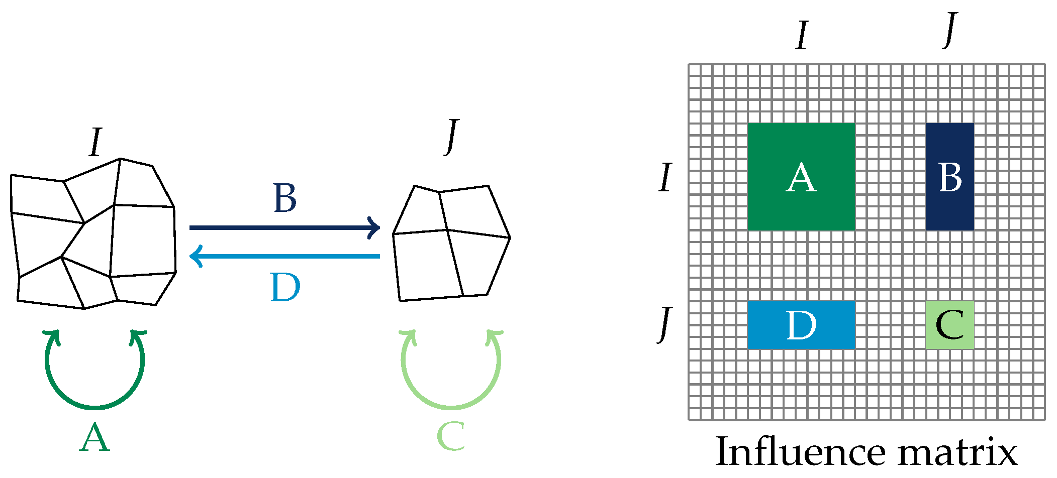
Each coefficient of the matrices corresponds to the interaction between two panels of the mesh. Then, each block of the coefficient in the matrix can be seen as the interaction between two sets of panels (see Figure 1).

Figure 1.
Schematic representation of the matrix blocks encoding the interaction between two sets of panels. A and C denote the interaction between a set of panels and itself, while B and D denote the interaction between the two sets of panels. The corresponding blocks B and D in the matrix might be approximated with low-rank matrices.
For distant sets of panels in the mesh, not all of the information contained in the block might be necessary. The main idea of the low-rank approximation is to compute some blocks only approximately and store them in a compressed way.
2.2.1. Introduction of Low-Rank Matrices
A low-rank matrix of size and of rank r (usually taken small with respect to N and M) is a matrix writable under the form , where A and B are matrices of sizes and , respectively. In particular, a matrix of rank 1 can be written as , where a and b are vectors and ⊗ denotes the tensor product.
The storage cost of a low-rank matrix of rank r is instead of . The multiplication of the matrix with a vector x of size M can be expressed as , that is, as scalar multiplications instead of . Thus, its use in an iterative linear solver can be faster.
2.2.2. Theoretical Study of Approximability with Low-Rank Matrices
Assuming that a kernel function has a separable expansion of the form
where for each k, and are any functions, then for any sets of points and , a matrix has a rank of at most r. To justify that off-diagonal blocks of can be approximated with low-rank matrices, it is then sufficient to show that the kernel function can be approximated with a separable expansion for distant x and y.
Instead of (13), the assumption that the kernel is “asymptotically smooth” as in (14) (see [13] Thm. 4.17 and 4.22) is a sufficient condition for the existence of a separable expansion that approximates M exponentially in r. More precisely, if
holds for some , with , , , , , and if x and y are -admissible, i.e.,
then there exists a separable expansion that approximates M with an error that decreases exponentially with r for that is small enough.
Unfortunately, the complexity of the explicit expressions of the Green function for linear potential flow (3) and (4) makes them difficult to prove (14). The (“simpler”) 3D Green function of the Helmholtz equation is a priori not asymptotically smooth at high frequencies [27]; nevertheless, in [28], a study of the approximability of the Helmholtz kernel, the following was shown:
- For a fixed frequency, the rank for a given wave number does not increase with the number of points by wavelength;
- For a fixed number of points by wavelength, the rank should not increase more than until it reaches the high-frequency regime where the block is not low-rank anymore.
Considering only the asymptotic expression (6), we expect a similar behavior because of the oscillating term , which is also the asymptotic approximation of the 2D Helmholtz kernel ([29] Eq. 9.2.3).
2.2.3. Numerical Methods for Compression
The optimal low-rank compression of any matrix can be constructed by truncating the singular value decomposition (SVD) of the matrix. However, the computation of the SVD can be costly, and other techniques are used in practice. The most common one is the Adaptive Cross-Approximation (ACA), which allows approximation to be built with only coefficients from the full matrix [30].
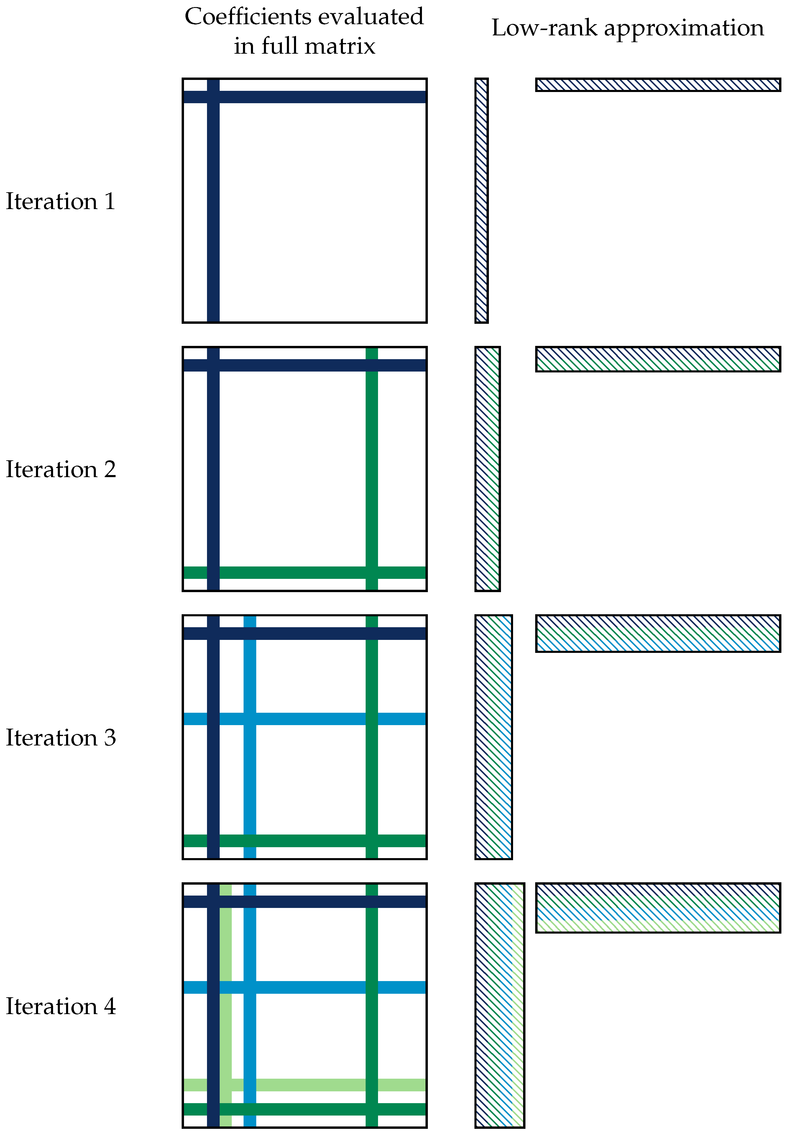
The ACA is a compression technique that iteratively builds a low-rank matrix by picking only one line and one column of the matrix at each iteration (see Figure 2). In the first step, a line and a column of the full matrix are picked arbitrarily (either chosen at random or arbitrarily fixed to be the top row and leftmost column, as in the numerical studies of Section 3) to build an approximation of rank one of the matrix. Then, at iteration , a new line and a new column are chosen based on the existing low-rank compression of rank n. They are added to the low-rank compression to build a low-rank compression of rank . The norm of the new matrix of rank is computed and compared to the previous one of rank . If the change in the norm is lower than a given threshold, the method is supposed to have converged.

Figure 2.
Schematics of the adaptive cross-approximation of a square matrix: on the left, the lines and columns that are evaluated in the full matrix; on the right, the assembly of a low-rank compression of rank 4. Note that the lines and columns in the low-rank compression do not have the same values as the lines and columns with the same color in the full matrix but are derived from them.
Note that not all of the coefficients of the full matrix are used. In practice, this means that the Green function needs only to be evaluated on the lines and the columns that are picked up. This is especially useful for linear potential flow problems since the Green function is costly to evaluate.
2.2.4. Structures of Matrices with Low-Rank Blocks
Matrices stemming from the discretization of boundary integral equations cannot generally be directly approximated with low-rank matrices, but sub-blocks corresponding to far interactions satisfying (15) can. There exist several data-sparse formats that incorporate low-rank approximations; they all have different theoretical complexities, and their implementation can be more or less involved.
The most common data-sparse format is the -matrix format; see [12,13]. It is based on a hierarchical partition of the physical domain: a cluster tree. The matrix can then be represented via a block tree corresponding to interactions between nodes in the cluster tree. To build the actual -matrix, the block tree is traversed as follows: Starting from the root block,
- if a block satisfies (15), it is compressed as described in Section 2.2.3;
- otherwise, we visit its children, unless their corresponding blocks are too small, in which case they are represented with a dense block.
One advantage of -matrices is that all of the usual matrix operations can be performed; for example, it can be used for a matrix–vector operation, and its cost is . However, due to its hierarchical nature, the implementation is not straightforward. Other formats exist; for example, -matrices, HOLDR, and block low-rank (BLR). In the following numerical experiments, we will also use the BLR format. It is very similar to the -matrix format but without the hierarchical clustering. Only one level of partition is used—in our case, each cluster corresponds to one object, and if two objects satisfy (15), their interaction is compressed. The BLR format was studied in [31,32].
3. Numerical Experiments
Given the complexity of the Green function for linear potential flow, the best way to assess the validity of low-rank compression is to experimentally test it in real conditions in an existing BEM solver. For this purpose, the open-source BEM solver Capytaine [17] was used.
Unless stated otherwise, all experiments were performed by computing the full expression of the Green function (4) and not by using the tabulation and the asymptotic expression (6).
3.1. Two Floating Hemispheres at Varying Distance
Let us consider two identical floating spheres with a diameter of 1 m, with their centers at the free surface, separated by a distance d, and discretized with N panels each. (Since only the immersed part of the body is discretized, the mesh is actually two half-spheres at distance d.) Unless stated otherwise, we consider a mesh resolution of panels, a wavelength of m, and a water depth of .
All interaction matrices S and K are of size and can be decomposed into four blocks: two diagonal blocks A encoding the interactions of a sphere with itself and two non-diagonal blocks B encoding the interactions of a sphere with the other. Since the spheres are identical, the blocks are actually identical, and the matrices have the following form:
For this numerical experiment, the non-diagonal blocks B are approximated with low-rank blocks of given rank r, , using either the singular value decomposition (SVD) or the adaptive cross-approximation (ACA). The resulting approximated matrix reads
The relative error of this approximation is evaluated as follows:
where denotes the Frobenius norm.
The same procedure is repeated for several distances d between the spheres. Each time, the relative error for each rank r is computed for both matrices S and K using both the SVD and the ACA.
3.1.1. Influence of the Distance and the Rank on the Error
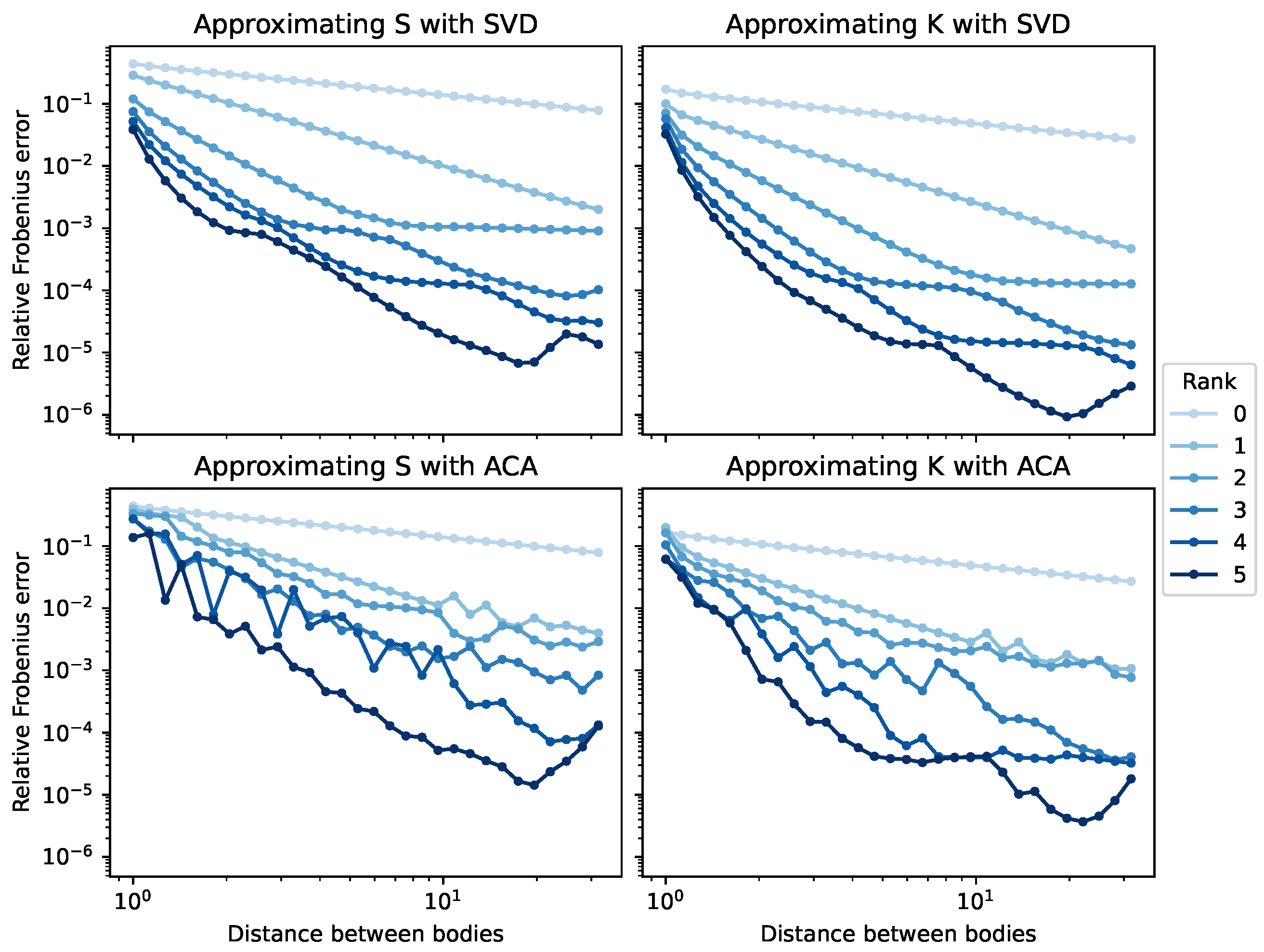
For the first experiment, we want to study the influence of the rank on the relative Frobenius error as a function of the distance. The results are presented in Figure 3.

Figure 3.
Relative Frobenius error between the full matrix and the low-rank compressed matrix as a function of the distance between the two bodies for two methods of low-rank compression (SVD and ACA) and with two BEM matrices (S and K) for varying ranks of the low-rank compression.
Firstly, as expected, the error of the low-rank compression decreases when the distance between the two spheres increases. The error also decreases when the rank of the low-rank compression matrix increases. A matrix of rank 0 (that is, a zero matrix that completely neglects the interaction between the two spheres) is a poor approximation. However, a matrix of rank 2 or 3 is sufficient to have an error of less than 1%. For a block, a compression of rank 2 stores 4% as many coefficients as the full block, meaning that we can reach 99% accuracy with less than 10% of the computation.
The errors in the compression of S and K are fairly similar. Both matrices are as difficult as the other to approximate with such a method.
Finally, we can check the efficiency of the ACA with respect to the optimal low-rank compression obtained with the SVD. The compression obtained from the ACA is noisier and slightly less accurate than that obtained with the SVD, but still decreases with the rank and the distance in the same way as that of the SVD.
3.1.2. Influence of the Distance and the Wavelength on the Error
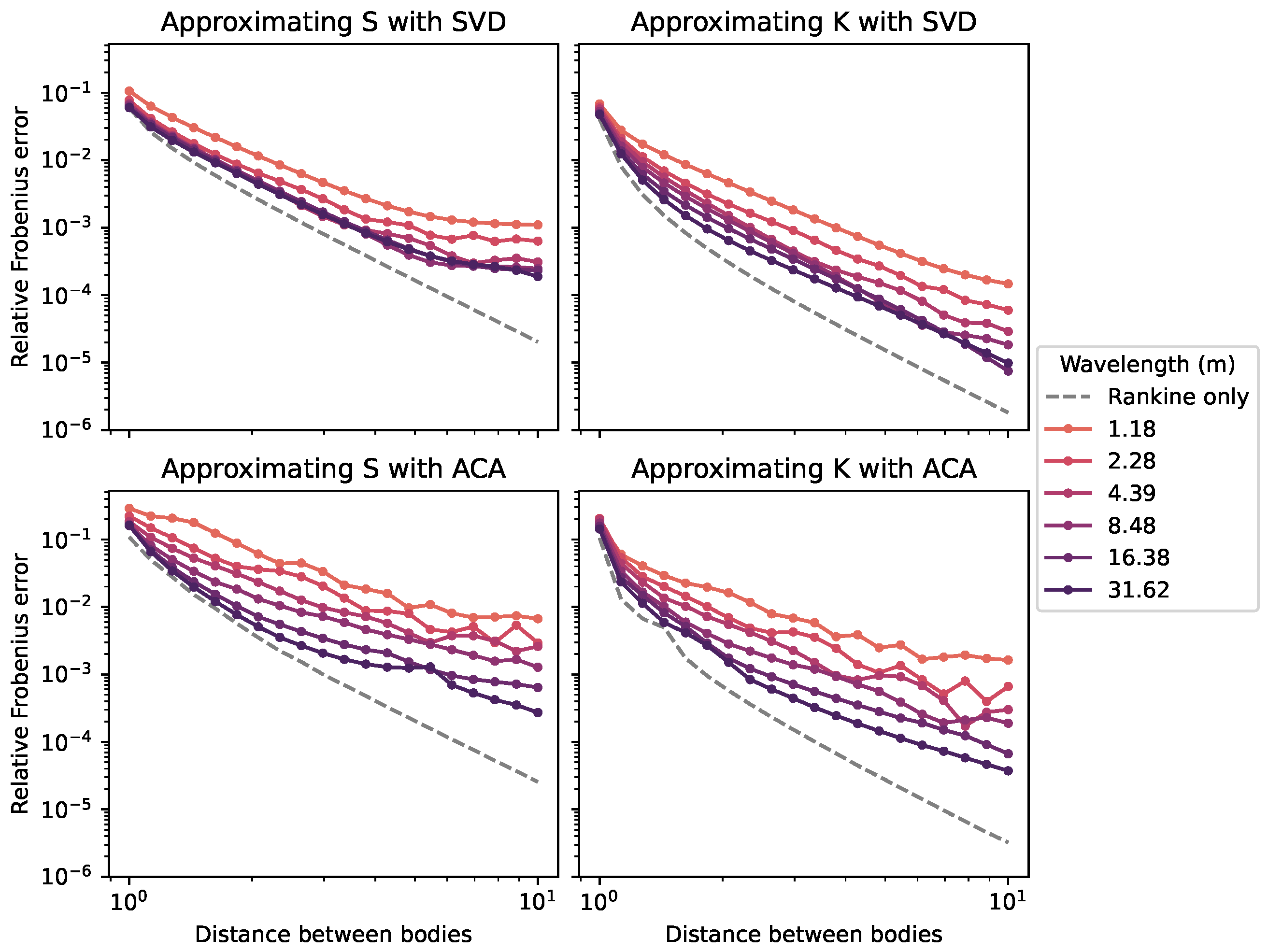
In this experiment, we study the influence of the wavelength. The rank of the low-rank compression is now fixed to 2, while several wavelengths between m and m are now tested. (Smaller wavelengths would require a finer mesh to be accurately captured.) The Rankine term of the Green function alone (that is, without the frequency-dependent wave term) is also tested. The results are presented in Figure 4.

Figure 4.
Relative Frobenius error between the full matrix and the low-rank compressed matrix as a function of the distance between the two bodies for two methods of low-rank compression (SVD and ACA) and with two BEM matrices (S and K) for several wavelengths (colored lines), as well as for the Rankine kernel (dashed gray line).
The most efficient compression is obtained when the Green function is only the Rankine kernel. For the full Green functions with a wave term, the error always decreases more slowly with the distance than for the Rankine term.
As expected from the discussion in Section 2.2.2, the compression is more efficient for long wavelengths, that is, low frequencies.
3.1.3. Influence of the Computation Method for the Green Function on the Error
Now, we study the role of the method used to compute the Green function. In the previous experiments, the exact expression of the Green function (4) was used. However, the default method in Capytaine is not to compute this costly exact expression, but instead to use approximations. For close panels, values are interpolated from a pre-computed table of exact expressions (4). For distant panels, the asymptotic expression (6) is used.
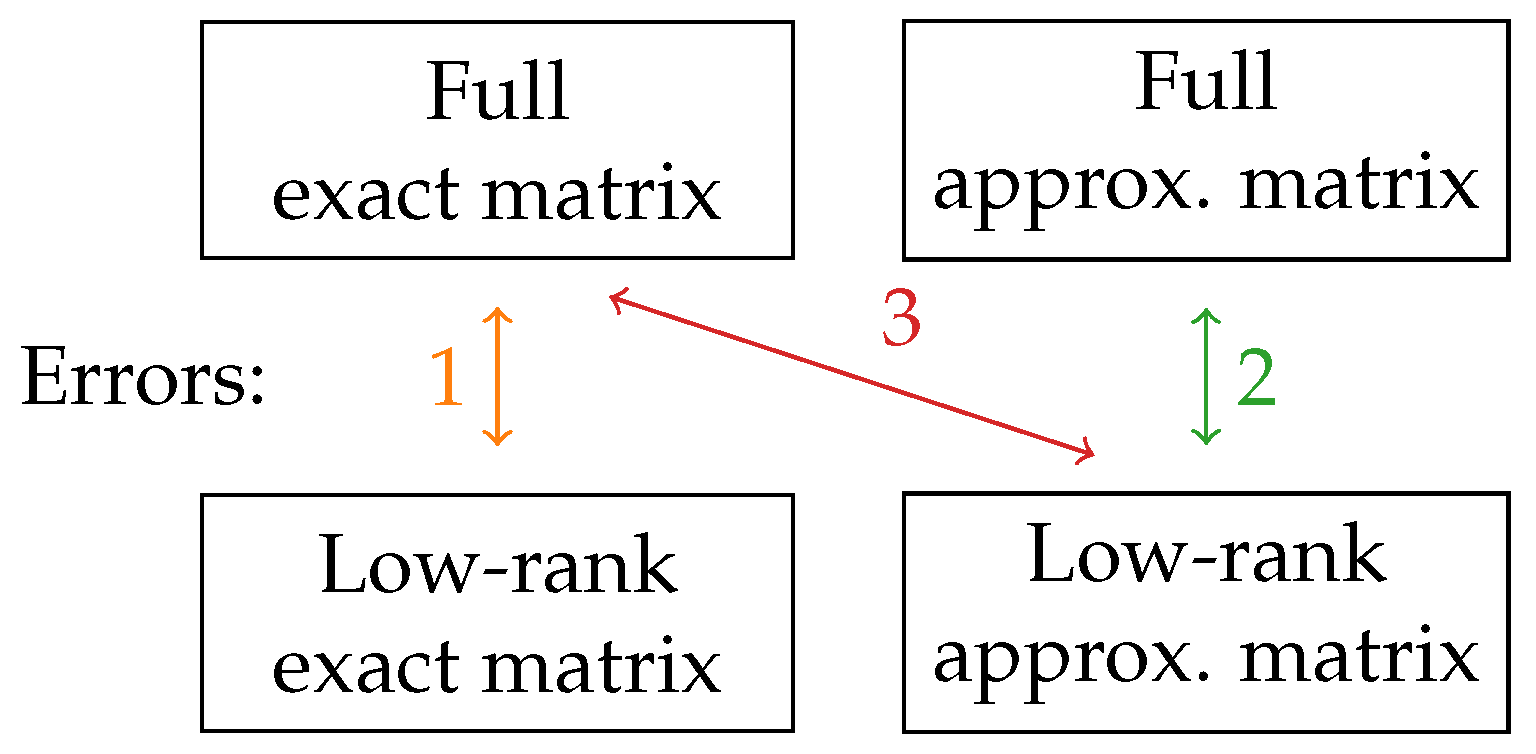
When introducing two independent ways to approximate the matrices, there are more ways to compute the error. In Figure 5, the three errors that we consider are summarized in a diagram. Error 1 is the error due to the low-rank compression of the matrix computed with the exact Green function (4), as presented in the previous graphs. Since the goal of this study is to evaluate the performance of the low-rank compression, we are interested in error 2, which is the error due to the low-rank compression when working with the approximate Green function. However, since the end goal would be to use both the low-rank compression and the Green function approximation, we also plot error 3, which incorporates the error due to the approximation of the Green function.
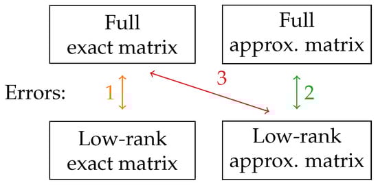
Figure 5.
Schematics of the different kinds of errors of the low-rank compression that can be computed when introducing an approximate expression for the Green function. Errors 1 and 2 only measure the effect of the low-rank approximation, but error 3 is the one that is actually relevant to the study of the accuracy of a BEM solver with low-rank compression.
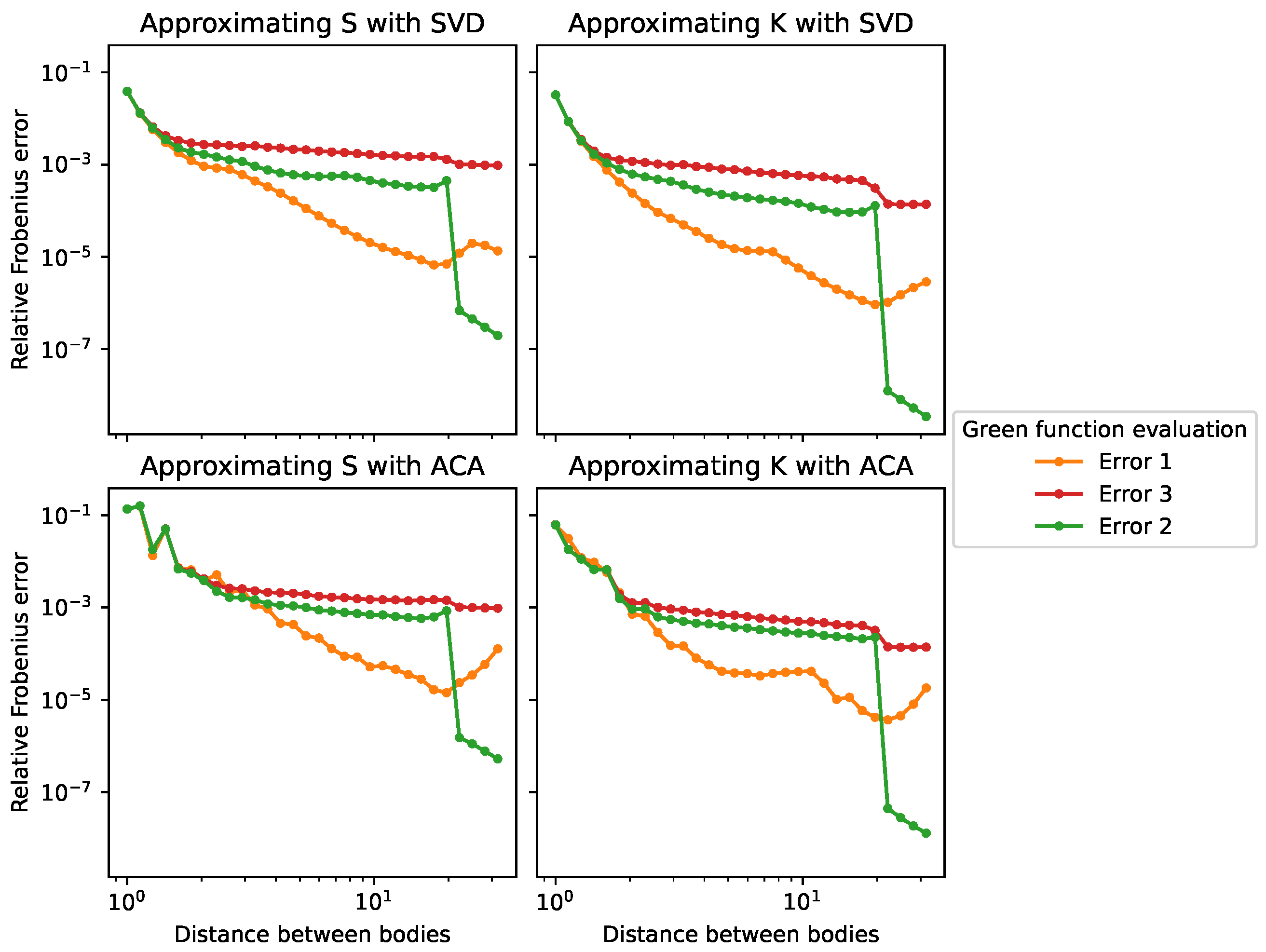
The results of the comparison of the exact and the approximate expressions are presented in Figure 6. Here, the rank of the compression is fixed to 5 (as the difference is less visible for lower ranks), and the wavelength is fixed to 1 m.

Figure 6.
Relative Frobenius error between the full matrix and the low-rank compressed matrix as a function of the distance between the two bodies for two methods of low-rank compression (SVD and ACA) and with two BEM matrices (S and K) for several methods of computation of the Green function, as described in Figure 5.
A jump is clearly visible in the error of the full approximate matrix with respect to the low-rank approximate matrix (error 2). This corresponds to the switch from the tabulated approximation to the asymptotic approximation, which occurs near . For distances below , the approximation of the tabulated Green function shows worse results than those of the exact Green function. One can suppose that the interpolation in the tabulation introduces spurious “information” in the matrix that is not accurately captured with the low-rank compression. On the contrary, for distances above , the approximation of the asymptotic Green function shows better results than those of the exact Green function. Similarly, one can suppose that the asymptotic expression contains less “information” than the exact Green function and is, thus, easier to compress with a low-rank block.
The errors due to both the compression and the approximation (error 3) are always higher. The use of an approximate formula for the Green function leads to relative errors of the order of . This means that it is useless to try to reach a low-rank compression error of less than when working with the approximate Green function, as the approximation will be the bottleneck. The tuning of Delhommeau’s approximation of the Green function as used in Capytaine is outside the scope of this study.
3.1.4. Influence of the Resolution on the Rank
In all of the previous experiments, the rank of the compression was fixed, and then the error was computed. In practice, the opposite is done: A tolerance is set on the error, and then the SVD or ACA searches for the lowest rank that allows the compression of the matrix block with such an error. In all test cases from now on, the tolerance will be fixed instead of the rank.
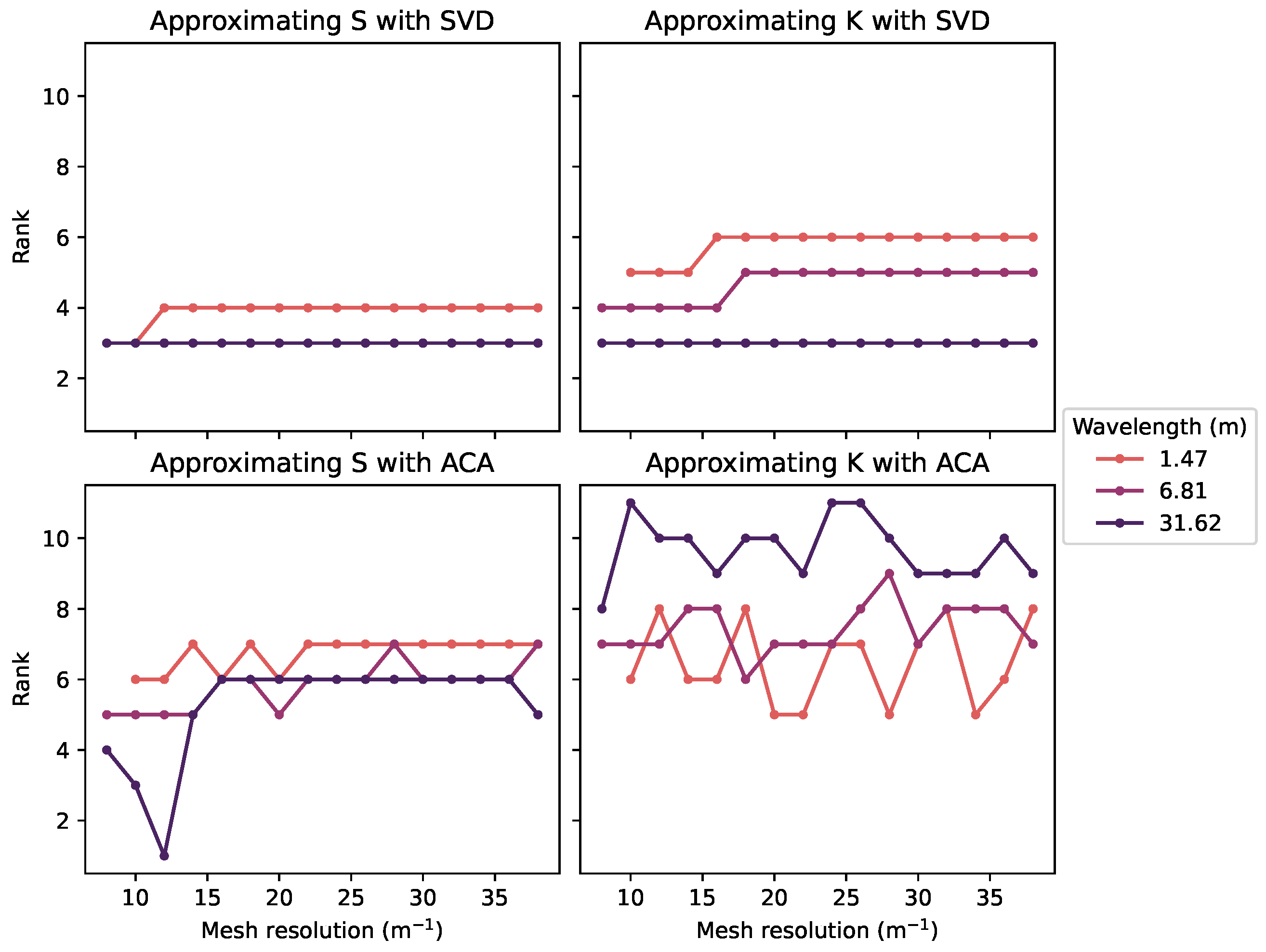
In this new test case, we experimentally test if the oscillatory kernel has the same behavior as that theoretically predicted by [28] for the Helmholtz equation. In particular, the influence of the resolution of the mesh on the rank of the approximation is studied. The distance is fixed to 4 , and the tolerance is fixed to . For several wavelengths and mesh resolutions (such that the mesh resolution is sufficient to capture waves of that wavelength), a low-rank approximation is built using the given tolerance.
The results are presented in Figure 7. As already noticed in Section 3.1.2, the lower-wavelength cases are harder to compress with low-rank blocks. As predicted in [28], the rank is basically constant as the mesh resolution increases when the approximation is computed with the SVD. The results of the ACA are noisier, but the same tendency can be assumed.

Figure 7.
Rank of the best low-rank compression for a given error threshold as a function of the mesh resolution for two methods of low-rank compression (SVD and ACA) and with two BEM matrices (S and K) for several wavelengths. Points for which the mesh resolution is insufficient for a given wavelength have been removed from the graph.
For a given geometry and a given wavelength, the rank of the approximation for a given error can be assumed to be constant with the resolution of the mesh. Consequently, the cost of the low-rank blocks only grows like with the number of panels N. In other words, providing a resolution that is too high for the desired accuracy will not be as much of a burden on the performance as it would be for a full matrix.
3.2. Array of Random Floating Spheres
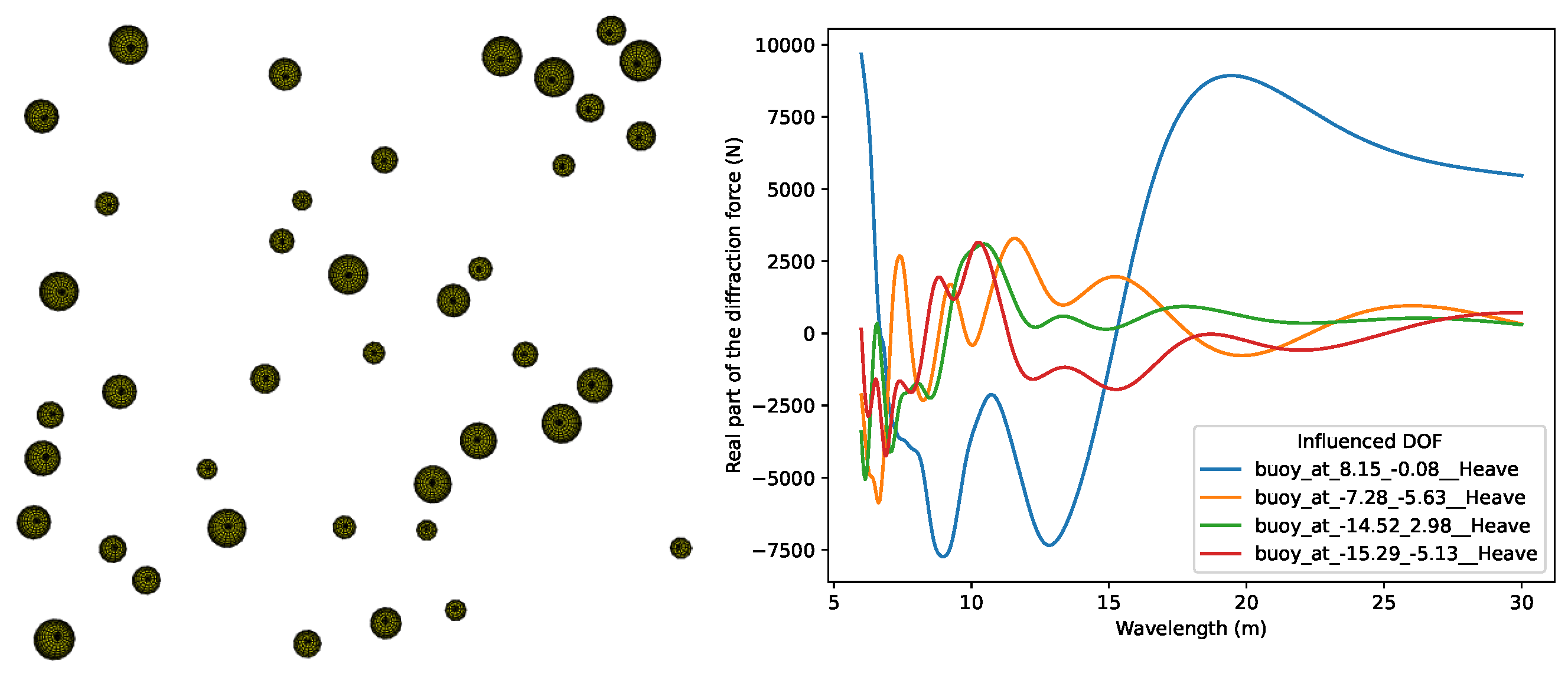
In this section, we introduce a new experiment that is closer to a real application. Forty hemispheres with random radii (between and 1 ) are positioned randomly on a free surface in a square with a size of . (When a collision between two spheres is detected, the random positioning algorithm is restarted until no collision is found). Depending on the size of the spheres, the full problem is composed of around 5000 panels, which is large enough to be worth approximating with low-rank blocks while being small enough to also be solvable with a full matrix with a reasonable amount of RAM (circa 750 with Capytaine’s default settings). See Figure 8 for a view of the mesh, as well as an example of result.

Figure 8.
(Left) example of a mesh with 40 spheres with random radii that are positioned at random. (Right) example of diffraction force on four of the spheres as a function of the wavelength.
The accuracy of the method is not computed on the matrix itself anymore, but rather on the physical output of the solver. For this purpose, the diffraction force on body i with respect to the Heave degree of freedom (that is, the vertical component of the diffraction force on the body) is chosen. The reference solution is computed using full matrices, and the relative error in the diffraction force is computed as
where is the diffraction force vector computed with the low-rank block compression, is the reference diffraction force vector, and is the infinite norm.
The range of wavelengths of interest is chosen to be between 6 and 30 . Lower wavelengths are not studied in order to avoid irregular frequencies appearing around wavelengths of 2 .
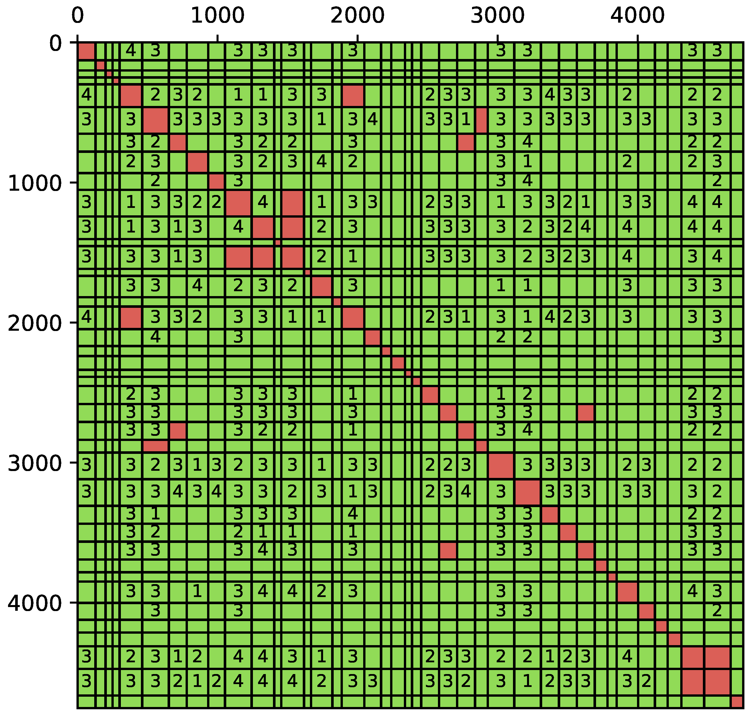
The interaction matrices can be seen as 40 block × 40 block matrices, where each block is the interaction between two of the hemispheres in the domain. A block in this matrix is computed with a low-rank approximation if the admissibility criterion (15) is satisfied, where is set here to . See Figure 9 for a graphical representation of such a matrix. When computing the low-rank approximation with the ACA, a tolerance on the error has to be set as a stopping criterion for the iterative process. A higher tolerance leads to sparser matrices with higher errors, and a lower tolerance leads to denser matrices with lower errors. Three different relative error tolerances are tested in this experiment: , , and .

Figure 9.
Structure of the resulting interaction matrix where red blocks are fully stored in memory, and the green blocks are low-rank blocks with a rank corresponding to the number displayed in the block.
Aside from the relative error in the diffraction force, the main output of interest is the density of the matrix, that is, the ratio of the number of coefficients stored in the matrix to the size of the matrix. The density of the reference method with a full matrix is 1. The density is strongly correlated with the gain in speed and memory of using the compressed matrix.
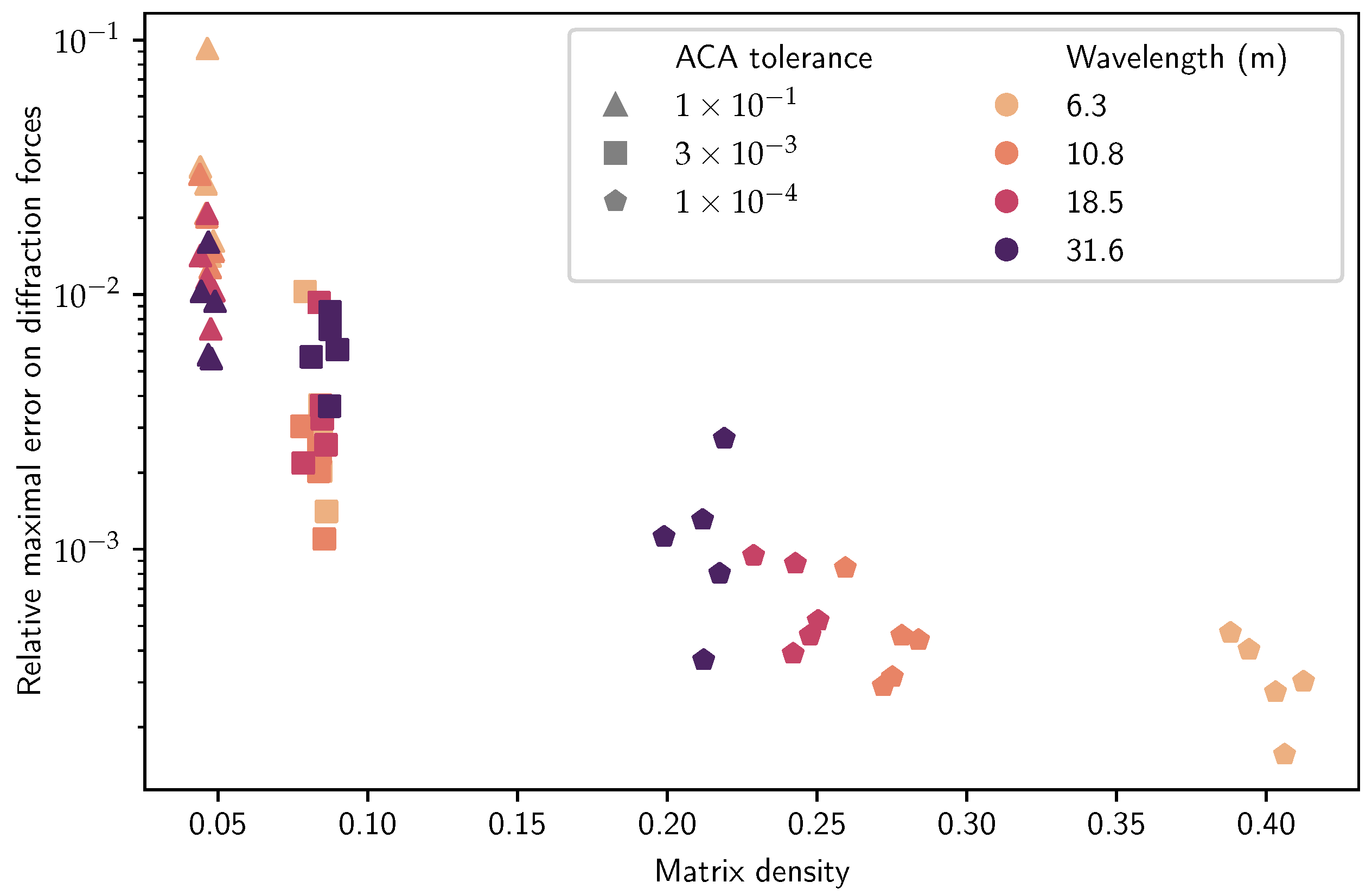
For each wavelength and each ACA tolerance, the simulation is repeated five times with different random generations of the array of floating spheres. The main results are presented in Figure 10. As expected, a lower tolerance in the ACA leads to a lower error and a denser matrix. By choosing a tolerance of , we observe that the error is below 1%, while the density of the matrix is around 10%. In other words, the solver reaches 99% accuracy with only 10% of the coefficients.

Figure 10.
For 60 simulations, the density of the matrix with low-rank blocks versus the relative error in the diffraction forces caused by the approximation of the matrix.
The effect of the wavelength is not as clear. With a lower tolerance , the higher frequencies (lower wavelength) seem to lead to denser matrices, which is consistent with the discussion in Section 3.1.2. With a higher tolerance, the wavelength does not have a clear effect on the result.
Note that with the block low-rank matrix structure (as illustrated in Figure 9), the complexity of the method is still , where is the number of bodies. The complexity could be reduced to by using a more complex block structure, such as the -matrix structure described in Section 2.2.4. The optimization of the matrix block structure is outside the scope of this study.
4. Discussion and Conclusions
This paper is about the suitability of low-rank approximation for linear potential flow. Due to the complexity of the expression of the Green function, the theoretical sufficient condition for compressibility with low-rank blocks could not be proved. Thus, we relied on numerical experiments to test the efficiency of the low-rank approximation.
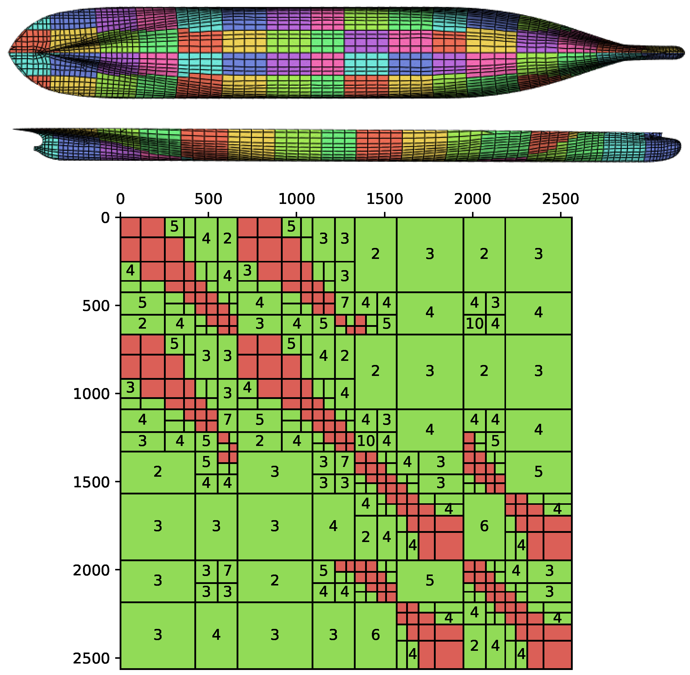
In the numerical examples presented in Section 3, the clusters of panels used to define the blocks of the matrix corresponded to disjointed bodies. This is the most natural way to split the mesh when studying problems such as those of farms of wave energy converters. However, having each cluster matching one and only one disjoint body is not a requirement of the method. For instance, a mesh with a single large floating body can be split into clusters of panels, and the interaction between these distant clusters can be approximated with low-rank blocks. An illustration is given in Figure 11, in which the mesh of a realistic ship (provided by the authors of [33]) is split into a hierarchical cluster of panels, which are used to build a -matrix. In this illustrative example of possible further applications, the matrices are approximated with a density of ∼21%, while the relative error on the heave component of the diffraction force is around 2%.

Figure 11.
(Above) Top and side view of the ship hull mesh, where the panels’ colors correspond to the 60 clusters of panels composing the mesh. (Below) Resulting -matrix for the S matrix with a density of ∼21%, where red blocks are fully stored in memory, and green blocks are low-rank blocks with a rank corresponding to the number displayed in the block.
Only infinite-depth results have been presented in this paper. Early tests with the finite-depth Green function showed similar efficiency for the low-rank approximation. However, the influence of the computation of the Green function, as presented in Section 3.1.3, would need to be reconsidered with the additional approximation that was performed to compute the finite-depth Green function with Delhommeau’s method [18].
The prototype implementation in Capytaine is available to all users of the code and can be used, e.g., to solve very large problems that would not otherwise fit in RAM. However, for most small- to medium-sized problems, its usage is not recommended, as it is often less performant than the default full-matrix method. This lower performance of the more advanced method can be explained by two main factors.
Firstly, the handling of matrices with low-rank blocks requires more bookkeeping than that required by plain full matrices. This is critical in the current implementation of Capytaine, as this bookkeeping is implemented in Python, which is a relatively slow programming language. The block low-rank structure was considered in Section 3 instead of -matrices with the hope of reducing this bookkeeping cost. Due to our naive implementation, this cost is still disproportionate, and for this reason, no time benchmark is presented in this paper. A solution would be to use another library with a low-level language as a dependency for dealing with the compression and to additionally use -matrices, which will also offer better performance in terms of complexity due to their hierarchical nature. Examples of such libraries are Hlib (http://hlib.org (accessed on 3 January 2024)), HiCMA (https://ecrc.github.io/hicma/ (accessed on 3 January 2024)), hmat-oss (https://github.com/jeromerobert/hmat-oss (accessed on 3 January 2024)), and Htool (https://htool-documentation.readthedocs.io (accessed on 3 January 2024)). The latter is developed by one of the authors. Due to the modular structure of Capytaine, it is possible to integrate this kind of library with it, with the main technical difficulty being the interface between the different programming languages involved.
Secondly, the low-rank block compression interferes with other optimizations used by Capytaine. As an example, the evaluation of the Green function for S and the evaluation of its derivative for K share much common code, and the two matrices are built together by Capytaine. Using matrix compressions would require coupling the compression of both matrices, which, to our knowledge, has never been done. Preliminary tests showed that the rows and columns chosen by the ACA for one of the two matrices gave satisfying results when approximating the second matrix.
Another example is the choice of the linear solver; the low-rank block prototype presented here used a GMRES solver. The default method in Capytaine is to compute the LU decomposition once and apply it for all of the right-hand sides associated with the matrix. When GMRES is used with the block low-rank approximation, it currently restarts the resolution of the linear system from scratch for each right-hand side. One possibility to overcome this issue is to factorize the block low-rank matrix, which can be done efficiently depending on the maximal rank. This approach was recently studied in the context of finite-element matrices [31,32]. Another possibility is to use the more involved -matrix format, which can also perform all matrix operations, unlike other data-sparse formats and, in particular, factorizations, while having even better theoretical complexities. Thus, to solve problems with multiple right-hand sides, a solution to avoid iterative solvers would be to use the approximate LU factorization associated with -matrices; see [13] (Section 7.6) or [12] (Section 2.7). An alternative solution would be to use a more efficient iterative solver, and, in the case of multiple right-hand sides, block iterative methods have been investigated (see [34] and [35] (Section 6.12)). Instead of solving each right-hand side separately, these methods solve them all at the same time using matrix–matrix operations, which is more efficient than several matrix–vector operations, and this allows a larger search space to be built. These methods are also usually coupled with recycling techniques to reuse some previous information built before a restart or in a previous solve; see [36,37,38]. Finally, the performance of the GMRES could be improved by the use of a good preconditioner [39].
Beyond low-rank compression, other data-sparse matrices can be used to reduce the computational cost of BEM solvers. For instance, the local symmetries of a mesh lead to Toeplitz-type matrix structures [40]. One can imagine coupling these optimizations to reduce the computational cost of BEM solvers for large problems even further in the future.
Author Contributions
Conceptualization, M.A.; methodology, M.A. and P.M.; software, M.A.; writing—original draft preparation, M.A. and P.M.; writing—review and editing, M.A., P.M. and F.D.; supervision, F.D.; funding acquisition, M.A. and F.D. All authors have read and agreed to the published version of the manuscript.
Funding
The work of M.A. was funded partly by Science Foundation Ireland (SFI) under Marine Renewable Energy Ireland (MaREI), the SFI Centre for Marine Renewable Energy Research (grant 12/RC/2302), and partly by the Alliance for Sustainable Energy, LLC, Managing and Operating Contractor for the National Renewable Energy Laboratory (NREL) for the U.S. Department of Energy.
Data Availability Statement
The source code for the figure presented in this paper is available at https://zenodo.org/doi/10.5281/zenodo.10362559 (accessed on 12 December 2023).
Acknowledgments
M.A. thanks Marco Gambarini for the helpful discussions.
Conflicts of Interest
Author Matthieu Ancellin was employed by the company Eurobios Mews Labs. The remaining authors declare that the research was conducted in the absence of any commercial or financial relationships that could be construed as a potential conflict of interest.
Abbreviations
The following abbreviations are used in this manuscript:
| ACA | Adaptive cross-approximation |
| BEM | Boundary element method |
| GMRES | Generalized minimal residual method |
| -matrix | Hierarchical matrix |
| LU decomposition | Lower–upper decomposition |
| RAM | Random-access memory |
| SVD | Singular value decomposition |
References
- Folley, M. Numerical Modelling of Wave Energy Converters: State-of-the-Art Techniques for Single Devices and Arrays; Academic Press: Cambridge, MA, USA, 2016. [Google Scholar]
- Ning, D.; Ding, B. Modelling and Optimization of Wave Energy Converters; CRC Press: Boca Raton, FL, USA, 2022. [Google Scholar]
- Babarit, A. On the park effect in arrays of oscillating wave energy converters. Renew. Energy 2013, 58, 68–78. [Google Scholar] [CrossRef]
- Göteman, M.; Giassi, M.; Engström, J.; Isberg, J. Advances and challenges in wave energy park optimization—A review. Front. Energy Res. 2020, 8, 26. [Google Scholar] [CrossRef]
- Singh, J.; Babarit, A. A fast approach coupling Boundary Element Method and plane wave approximation for wave interaction analysis in sparse arrays of wave energy converters. Ocean Eng. 2014, 85, 12–20. [Google Scholar] [CrossRef]
- Fàbregas Flavià, F.; McNatt, C.; Rongère, F.; Babarit, A.; Clément, A. A numerical tool for the frequency domain simulation of large arrays of identical floating bodies in waves. Ocean Eng. 2018, 148, 299–311. [Google Scholar] [CrossRef]
- Liu, Y.; Zheng, S.; Liang, H.; Cong, P. Wave interaction and energy absorption from arrays of complex-shaped point absorbers. Phys. Fluids 2022, 34, 097107. [Google Scholar] [CrossRef]
- Utsunomiya, T.; Watanabe, E. Accelerated higher order boundary element method for wave diffraction/radiation problems and its applications. In Proceedings of the Twelfth International Offshore and Polar Engineering Conference, Kitakyushu, Japan, 26–31 May 2002; International Society of Offshore and Polar Engineers: Mountain View, CA, USA, 2002. [Google Scholar]
- Fochesato, C.; Dias, F. A fast method for nonlinear three-dimensional free-surface waves. Proc. R. Soc. A Math. Phys. Eng. Sci. 2006, 462, 2715–2735. [Google Scholar] [CrossRef]
- Borgarino, B.; Babarit, A.; Ferrant, P. An implementation of the fast multipole algorithm for wave interaction problems on sparse arrays of floating bodies. J. Eng. Math. 2012, 77, 51–68. [Google Scholar] [CrossRef]
- Nokob, M.H.; Yeung, R.W. A fast multipole boundary element method for the three dimensional linear water wave-structure interaction problem with arbitrary bottom topography. Eng. Anal. Bound. Elem. 2020, 117, 232–241. [Google Scholar] [CrossRef]
- Bebendorf, M. Hierarchical Matrices; Springer: Berlin/Heidelberg, Germany, 2008. [Google Scholar]
- Hackbusch, W. Hierarchical Matrices: Algorithms and Analysis; Springer: Berlin/Heidelberg, Germany, 2015. [Google Scholar]
- Xie, C.; Choi, Y.; Rongère, F.; Clément, A.H.; Delhommeau, G.; Babarit, A. Comparison of existing methods for the calculation of the infinite water depth free-surface Green function for the wave–structure interaction problem. Appl. Ocean Res. 2018, 81, 150–163. [Google Scholar] [CrossRef]
- Korsmeyer, T.; Phillips, J.; White, J. A precorrection-FFT algorithm for accelerating surface wave problems. In Proceedings of the 11th IWWWFB, Hamburg, Germany, 17–20 March 1996. [Google Scholar]
- Jiang, S.c.; Teng, B.; Gou, Y.; Ning, D.z. A precorrected-FFT higher-order boundary element method for wave–body problems. Eng. Anal. Bound. Elem. 2012, 36, 404–415. [Google Scholar] [CrossRef]
- Ancellin, M.; Dias, F. Capytaine: A Python-based linear potential flow solver. J. Open Source Softw. 2019, 4, 1341. [Google Scholar] [CrossRef]
- Delhommeau, G. Problèmes de Diffraction-Radiation et de Résistance des Vagues: Étude Théorique et Résolution Numérique par la Méthode des Singularités. Ph.D. Thesis, École Nationale Supérieure de Mécanique de Nantes, Nantes, France, 1987. [Google Scholar]
- Babarit, A.; Delhommeau, G. Theoretical and numerical aspects of the open source BEM solver NEMOH. In Proceedings of the 11th European Wave and Tidal Energy Conference (EWTEC2015), Nantes, France, 6–11 September 2015. [Google Scholar]
- Alouges, F.; Aussal, M. FEM and BEM simulations with the Gypsilab framework. Smai J. Comput. Math. 2018, 4, 297–318. [Google Scholar] [CrossRef]
- Neumann, M. Hierarchical Matrices, An Implementation in Python. Master’s Thesis, University of Zurich, Switzerland, 2017. [Google Scholar]
- Babarit, A. L’énergie des Vagues: Ressource, Technologies et Performance; ISTE Group: London, UK, 2018. [Google Scholar]
- Newman, J.N. Marine Hydrodynamics; The MIT Press: Cambridge, MA, USA, 2018. [Google Scholar]
- Viswanathan, S.; Holden, C.; Egeland, O.; Greco, M. An Open-Source Python-Based Boundary-Element Method Code for the Three-Dimensional, Zero-Froude, Infinite-Depth, Water-Wave Diffraction-Radiation Problem. Model. Identif. Control 2021, 42, 47–81. [Google Scholar] [CrossRef]
- Molin, B. Offshore Structure Hydrodynamics; Cambridge University Press: Cambridge, UK, 2022. [Google Scholar]
- Saverin, J.R.; Grüter, L. Quadrature Schemes for the Integration of the Free-Surface Green’s Function within the Open-Source Boundary Element Method Library BEMUse. In Proceedings of the International Conference on Offshore Mechanics and Arctic Engineering. American Society of Mechanical Engineers, Hamburg, Germany, 5–11 June 2022; Volume 85925, p. V007T08A057. [Google Scholar]
- Banjai, L.; Hackbusch, W. Hierarchical matrix techniques for low- and high-frequency Helmholtz problems. IMA J. Numer. Anal. 2007, 28, 46–79. [Google Scholar] [CrossRef]
- Chaillat, S.; Desiderio, L.; Ciarlet, P. Theory and implementation of H-matrix based iterative and direct solvers for Helmholtz and elastodynamic oscillatory kernels. J. Comput. Phys. 2017, 351, 165–186. [Google Scholar] [CrossRef]
- Abramowitz, M.; Stegun, I.A. Handbook of Mathematical Functions with Formulas, Graphs, and Mathematical Tables; National Bureau of Standards Applied Mathematics Series 55; Tenth Printing; US Government Printing Office: Washington, DC, USA, 1972. [Google Scholar]
- Bebendorf, M.; Rjasanow, S. Adaptive low-rank approximation of collocation matrices. Computing 2003, 70, 1–24. [Google Scholar] [CrossRef]
- Amestoy, P.; Ashcraft, C.; Boiteau, O.; Buttari, A.; L’Excellent, J.Y.; Weisbecker, C. Improving Multifrontal Methods by Means of Block Low-Rank Representations. SIAM J. Sci. Comput. 2015, 37, A1451–A1474. [Google Scholar] [CrossRef]
- Amestoy, P.; Buttari, A.; L’Excellent, J.Y.; Mary, T. On the Complexity of the Block Low-Rank Multifrontal Factorization. SIAM J. Sci. Comput. 2017, 39, A1710–A1740. [Google Scholar] [CrossRef]
- Donatini, L.; Herdayanditya, I.; Verao Fernandez, G.; Pribadi, A.B.K.; Lataire, E.; Delefortrie, G. Implementation of forward speed effects on an open source seakeeping solver. In Proceedings of the 6th MASHCON: International Conference on Ship Manoeuvring in Shallow and Confined Water, Knowledge Centre for Manoeuvring in Shallow and Confined Water, Glasgow, UK, 22–26 May 2022; pp. 20–33. [Google Scholar]
- Simoncini, V.; Gallopoulos, E. Convergence properties of block GMRES and matrix polynomials. Linear Algebra Appl. 1996, 247, 97–119. [Google Scholar] [CrossRef]
- Saad, Y. Iterative Methods for Sparse Linear Systems; Society for Industrial and Applied Mathematics: Philadelphia, PA, USA, 2003. [Google Scholar] [CrossRef]
- Morgan, R.B. Restarted block-GMRES with deflation of eigenvalues. Appl. Numer. Math. 2005, 54, 222–236. [Google Scholar] [CrossRef]
- Agullo, E.; Giraud, L.; Jing, Y.F. Block GMRES Method with Inexact Breakdowns and Deflated Restarting. SIAM J. Matrix Anal. Appl. 2014, 35, 1625–1651. [Google Scholar] [CrossRef]
- Jolivet, P.; Tournier, P.H. Block Iterative Methods and Recycling for Improved Scalability of Linear Solvers. In Proceedings of the SC ’16: Proceedings of the International Conference for High Performance Computing, Networking, Storage and Analysis, Salt Lake City, UT, USA, 13–18 November 2016. [Google Scholar]
- Ciaramella, G.; Gambarini, M.; Miglio, E. A Preconditioner for Free-Surface Hydrodynamics BEM. In Proceedings of the 27th International Conference on Domain Decomposition Methods, Prague, Czech Republic, 25–29 July 2022; Available online: http://www.ddm.org/DD27/proceedings/015_13_BEM_precond-edited.pdf (accessed on 3 January 2024).
- Ancellin, M.; Dias, F. Using the floating body symmetries to speed up the numerical computation of hydrodynamics coefficients with Nemoh. In Proceedings of the ASME 2018 37th International Conference on Ocean, Offshore and Arctic Engineering (OMAE2018), Madrid, Spain, 17–22 June 2018; p. V009T13A031. [Google Scholar] [CrossRef]
Disclaimer/Publisher’s Note: The statements, opinions and data contained in all publications are solely those of the individual author(s) and contributor(s) and not of MDPI and/or the editor(s). MDPI and/or the editor(s) disclaim responsibility for any injury to people or property resulting from any ideas, methods, instructions or products referred to in the content. |
© 2024 by the authors. Licensee MDPI, Basel, Switzerland. This article is an open access article distributed under the terms and conditions of the Creative Commons Attribution (CC BY) license (https://creativecommons.org/licenses/by/4.0/).