Abstract
The purpose of this study was to enhance electric scooter performance utilizing a novel method consisting of an artificial neural network (ANN) and genetic algorithm (GA) to predict power demand, battery voltage, and identify the optimal performance range. For training, validation, and testing, a dataset comprising 1000 data points for each parameter was extracted from a MATLAB-Simulink model. The ANN application was used to identify the battery voltage and power demand, reflecting the simulated results under varying key input parameters. Additionally, the GA was used to identify the optimal performance after the ANN had been trained. The results showed that the ES can achieve a speed of 28.2 km/h while using an optimal power of 553 W, at a wind velocity of 0 m/s, a slope ratio of 0%, and a wheel diameter of 0.37 m. The achieved results show that the ANN-GA method is appropriate for determining the operating and structural parameters for maximizing the performance of electric scooters. To support the simulated results, an experimental study was carried out with an actual road test along the Taehwa river.
1. Introduction
Climate change has recently emerged as a problem for both the planet and many nations [1,2]. Air pollution, in particular the toxic emissions produced by internal combustion engines running on diesel and gasoline, such as hydrocarbons (HC), particulate matter (PM), nitrogen oxides (NOx), carbon monoxide (CO), carbon dioxide (CO2) [3,4], is one of the most important causes of climate change. Energy security, specifically the fluctuation in gasoline prices that recently hit a record high, is another crucial problem [5,6]. Due to the fluctuation of fuel prices as well as air pollution in urban cities, the electric scooter is emerging a promising solution to solve public mobility in crowded cities and densely populated areas [7,8]. Electric scooters are a different type of micro-mobility that have rapidly became popular their introduction in 2017 because of their outstanding advantages when traveling short distances, providing convenient mobility in urban areas [9]. However, the fast-growing usage, and the fact that the ES must operate at lower speeds than motor vehicle (for example, the legal maximum speed is 25 km/h in Europe), mean that the electric scooter operates ineffectively in terms of performance [10]. A detailed investigation of the key input parameters and their effects on dynamic and consumed energy will enable the improved performance/cost operation of electric scooter. This work proposes a combined ANN and GA to enhance performance as well as to optimize the consumed energy of electric scooters when operating at lower speeds in order to improve operation costs and extend battery life.
Research on electric scooter dynamics has been conducted. Chergui Hicham et al. conducted a study on the torque control of three-wheel electric scooter. The study applied a space vector modulation to control the torque of the wheel motor, which connects the scooter stability control system and energy storage system. The research results showed that the state of the battery can achieve more than 0.2% in 18 s [11]. Muhammad Nur Yuniarto et al. created an energy consumption model for an electric scooter. The study included various parameters such as scooter mass, scooter frontal areas, tire dimensions, and tire rolling resistance to estimate vehicle performance. The results demonstrated that the energy consumption prediction had errors of −8.63% and −4.7% when the experimental study was carried using a dynamometer and normal on-road testing [12]. In addition, Christina M.R. Garman et al. installed sensors on an electric scooter to measure acceleration, velocity, steering angle, and roll angle. The study evaluated accelerating, decelerating, turning, stopping, and unexpected braking events. Results showed that the e-scooter had a maximum lean angle of 59 degrees and a maximum lean rate of 783 deg/s [13]. Along with research about electric scooter performance, studies related to energy storage and battery charging to improve the flexible characteristics of electric scooters have been conducted. Jia-Sheng Hu et al. proposed a hybrid energy storage system using wireless power transfer for electric scooters to improve battery performance and extend the lifetime of the energy system. The study found that the efficiency of the overall system from the direct current source to the super capacity and battery is 86.4%, which was also confirmed by the experimental results [14]. Moreover, Paolo Di Giorgio et al. combined a battery pack and hydrogen tank to create a hybrid energy storage system that harnessed the endothermic nature of hydrogen desorption in metal hydrides to passively control the temperature of the battery [15]. Many studies have been carried out to investigate the charging of shared electric scooters. Rui Zhu et al. proposed a solar integrated charging station, with a real time shareability network to address the issue of shared e-scooters. By optimizing the PV size-reservation time, the system requires only a small percentage of the initial charging trips and PV modules (1–3 m2) to serve nearly 100% of user trips [16]. Alberto Martínez-Navarro et al. presented a stand-alone PV system as an ES recharging dock. The experimental test showed that the ES recharging dock provided additional autonomy with a distance of 31.2 km [17]. Moreover, to improve charging efficiency for solar charging system, Fatih Issi et al. proposed a class-e inverter for solar charging systems. However, the inverter output voltage varied with changes in the number of e-scooters being charged and a PID controller was used to keep the inverter output load voltage constant [18]. Furthermore, Muhammad Awais et al. presented an environmental impact study of a solar-powered charging station for electric scooters, demonstrating that the station can limit CO2 emissions by nearly 1154.21 kg/year [19]. A brief summary of studies in the area of electric scooters include approaches to improving stability control, energy consumption, acceleration, braking, the use of solar power transfer to enhance battery performance and extend the lifetime of energy systems, and environmental aspects such as limiting CO2 emissions. However, very few studies have considered the performance of electric scooters and methods to improve performance. This paper applies an ANN-GA method that used prediction and optimization to determine optimal performance for electric scooters. The ANN_GA method was used to predict and enhance the power demand and energy consumption of electric scooters under various operating and structure parameters.
Power demand and electric consumption are significant factors due to their influence on ES performance and the factors correlating with ES design and operations, such as wheel diameter, frontal area, slope ratio, and rider weight. The model’s ability to forecast power demand, battery voltage, and identify effective performance ranges showcases its potential to revolutionize the design and operation of electric scooters. Results from the ES Simulink model were used into validate, train, and test the ANN model. By using the appropriate operating and structural factors, the ANN-GA approach optimized the battery voltage and necessary power. The findings demonstrate that, at a slope ratio of 0%, a wheel diameter of 0.37 m, and a wind velocity of 0 m/s, the ES may reach an effective performance region at a speed of 28.2 km/h with an optimal necessary power of 553 W.
2. Data Generation for Machine Learning
2.1. Experimental Setup
The experimental test was carried out under the following circumstances. The rider weighed 77 kg, the wheel radius was 0.125 m, and the weight of the ES was 18 kg. The test was conducted for 60 s at Taehwa River on an actual road. The slope ratio of the road was practically 0%, and the wind velocity was nearly 0 m/s. The details of the ES experimental system utilized in the actual test are listed in Table 1. The experimental system for the electric scooter is shown in Figure 1. It consists of a variety of parts, including a computer, a lithium-ion battery (LIB), a DC motor, an NI-9221 module, a photo sensor, and an electric control unit. The DC motor was placed on the back wheel to produce the propulsion force, and an LIB was mounted on the scooter’s frame. A LabVIEW 2012 program installed on the computer allowed for the experimental data from the ECU module to be gathered and stored. A photo sensor monitored the motion of the wheel while the electric scooter was running and sent a digital signal to the ECU module to calculate the scooter’s speed. Additionally, the real-time voltage of the LIB was monitored using an NI-9221 module with an 800 kS/s sample rate. The LabVIEW program was used to monitor and record all the aforementioned signals after they had been transferred to the computer via a USB cable [20].

Table 1.
The electric scooter specifications.
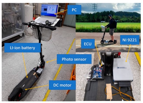
Figure 1.
The ES experimental system.
2.2. Simulation Study
Electric scooter dynamics
Figure 2 presents the free-body diagram of the ES. Newton’ second law was applied to simulate the ES’s motion. It is presented as the following equation:
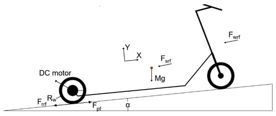
Figure 2.
The body diagram of ES.
The propulsion torque is calculated based on the wheel radius and propulsion force, as shown Figure 2.
When an electric motor is installed on the electric scooter (ES), as illustrated in Figure 2, the propulsion torque is represented using the following equation:
An electric motor, which can be mounted on the back wheel, is used by an electric scooter (ES). During ES operation, an electric motor produces propulsion torque to overcome numerous obstacles like friction, slope, and wind resistance. The electric motor dynamics are mathematically modeled by Equations (8) and (9) [21].
The electric motor’s armature current is an electrical variable, whereas the velocity is a mechanical variable. According to Equations (8) and (9), it can be deduced that the back electromotive force EMF (Ec) is proportional to the speed, and the generated torque (Te) is proportional to the armature current. This relationship is expressed by Equations (10) and (11), as follows:
The dynamics of the electric motor can be represented by substituting Equations (10) and (11) with Equations (8) and (9). This is demonstrated by the following Equations (12) and (13):
Equation (7) can be used to approximate the propulsive force of the ES in Equations (14) and (15). The expression, as a result, is as follows:
The propelling force could be simplified and represented by the equations above by combining Equations (14) and (15):
and the torque of propulsion could be expressed using the bellowed equation:
Performance of ES
The total power utilized to propel an ES and driver and overcome friction, slope, and air resistance is given by the equation below:
Based on the total power consumed (Ptotal), the power of an electric motor (Pm) to assist the rider while pedaling was chosen. The flowchart in Figure 3 outlines the calculation procedure for calculating the required power (Prq) of the electric scooter. The frontal area (A(i)) and slope grade (G(i)) are examples of input parameters, with index ‘i’ standing for each individual input parameter.
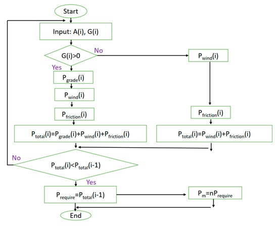
Figure 3.
The considered power flowchart of the ES.
The law of conversation energy states that the total energy intake equals the total energy output plus the total energy loss, which are calculated using Equation (22) below:
Energy Consumption Model
The battery model has a total capacity of 10 Ah and an open voltage terminal of 36 V. The energy consumption equation can be calculated by the following [22]:
where PBatt.Loss is the lost battery power due to internal resistance; therefore, the above equation can be explored as follows:
Based on Equations (26) and (27), the total available energy in the battery can be represented by the following equation:
It(t) is the nominal energy-specific accommodate in the battery. It is assumed to be constant when the battery has a nominal voltage. Thus, the total used energy can be expressed by Equations (29) and (30) below:
A MATLAB/Simulink model was created using Equation (1) through (30). The model’s objective was to test and assess the electric scooter’s performance traits and energy usage.
3. Machine Learning
3.1. Artificial Neural Network Fundamental
Machine learning approaches including artificial neural networks (ANN) are effectively utilized for tasks such as pattern recognition, classification, regression, and prediction. Inspired by the design and operation of biological neural networks in the brain, a neural network has several layers, including output, hidden, and input layers. Each layer contains a specific number of neurons. The neurons perform two main functions: the summation function, which calculates weighted inputs, and the activation function, which processes this sum to generate the neuron’s output. Information flows unidirectionally through the network, moving from the input layer to the output layer. Every layer receives signals from the neurons of the layer above and sends its own output to the layer above. Backpropagation (BP) neural networks propagate the cumulative error between the final network output and the actual value, which is frequently determined using experimental data [23]. This backward propagation enables the adjustment of weight values throughout the entire network mechanism. Figure 4 presents a visual representation of this process.
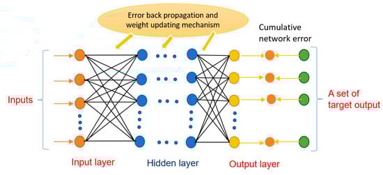
Figure 4.
The artificial neural network using multi-layer feedforward architecture.
Artificial neural networks (ANNs) provide faster predictions than conventional simulation programs [24]. Neurons, which are interconnected processing nodes in ANNs, accept input from outside sources, aggregate it, perform a nonlinear operation on it, and then produce an output. The feedforward network, which has an input layer, an output layer, and numerous hidden layers, is a well-known ANN model. Each neuron in the network has weighted inputs and outputs, allowing for flexible information processing [25]. The process of adjusting the weights between network layers to achieve the desired outcome is known as “training” the network. The output equation can be presented by the following:
Three basic criteria are frequently employed in assessing and optimizing artificial neural network (ANN) models. First, the key criterion is chosen to be the least mean square error (MSE) during the validation phase, as indicated in Equation (32). Second, if possible, efforts are made to reduce the complexity and size of the network. Finally, the regression between the output of the network and the related targets is evaluated by determining a correlation coefficient (R2), which is described in Equation (33). The correlation coefficient ranges between 0 and +1, where values closer to +1 indicate a strong positive linear correlation, while values closer to 0 indicate a weak correlation. Choosing the network configuration with the least MSE during validation is given priority when determining the hidden neuron numbers [26,27]. However, the other two criteria are also important for a comprehensive evaluation.
3.2. Development of ANN Model
The development of the predicted model was performed in MATLAB 2021 software. It was preceded by selecting the optimal configuration that achieved the lowest mean squared error (MSE) and a robust correlation coefficient (R value). The Levenberg–Marquardt algorithm was employed to expedite the training process of the model. The experimental dataset was partitioned into three subsets: validation, testing, training data. These subsets encompassed 70%, 15%, and 15% of the total dataset. The artificial neural network (ANN) was designed with a basic structure comprising two input variables and three output variables, along with a single hidden layer. The key parameters included the wheel radius (Rw), the scooter velocity (V), wind speed (Vw), rider mass (Mr), and slope ratio (G), which were used as the input factors. The required power and battery voltage were used as the output parameters, as shown in Table 2. According to Table 2, the quantity of neurons for the input and output layer are 5 and 2, while the quantity of neurons for the hidden layer need to be optimized. To ascertain the ideal quantity of hidden neurons, a sensitivity analysis was conducted to examine the relationship between MSE and R2 values and the quantity of hidden neurons. The trained network model was utilized to assess the fluctuation of MSE with respect to the quantity of hidden neurons, which is shown in Figure 5. The largest correlation coefficient (R2) between the actual and predicted value during validation stage was 0.998 with 12 hidden neurons. The MSE was minimized (0.003) at 12 hidden neurons. The architecture of the ANN model used in this analysis was configured as 5-12-2, indicating 5 input neurons, 12 hidden neurons, and two output neurons, as shown Figure 6. This configuration yielded satisfactory results, as evidenced by the favorable fit observed in the regression plots.
Table 2.
The selected ANN network was generated by the MATLAB framework.
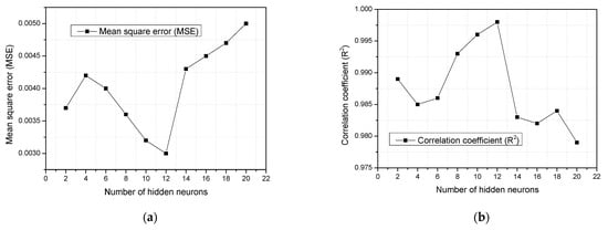
Figure 5.
Variation of MSE and R2 with regard to the amount of hidden neurons: (a) mean square error (MSE); and (b) correlation coefficient (R2).
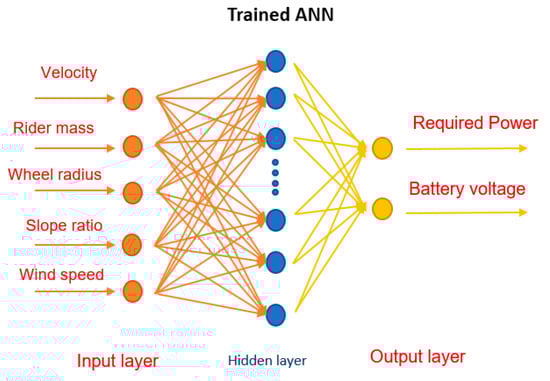
Figure 6.
Recognized ANN structure of 5-12-2.
3.3. Genetic Optimization Algorithm
The optimization method known as a genetic algorithm (GA) takes cues from genetics and natural selection. To solve a problem, it generates a population of alternative solutions and iteratively develops them over several generations. The components typically found in the design of a genetic algorithm include a population of chromosomes or individuals, a fitness function used to assess the fitness or appropriateness of each prospective solution, a selection operator that picks individuals from the population as parents for the subsequent generation, crossover and mutation operators for generating new individuals in the next generation, and termination criteria that define when the algorithm should conclude.
An n-dimensional chromosome is a data structure that provides a prospective answer to an issue in the context of a genetic algorithm. It consists of n genes, where each gene represents a choice varying in the solution space. In this case, the chromosome can be expressed using the following equation [28]:
where ci is the i-th value of parameters, n is the gene number. There are five parameter values in this research, including: wheel radius (Rw), scooter velocity (v), mass (M), slope ratio (G), and wind velocity (Vw). To reach an optimization target, power demand and voltage were chosen as elements in the ANN-GA approach, with details as follows.
In order to solve the optimization problems, the fitness function is utilized to assess each chromosome’s quality, and genetic operators like crossover and mutation, are used to create new offspring chromosomes. In this instance, the chromosomal possibility yielding the optimal necessary power can be expressed as follows [28,29]:
where: N is the number of parent chromosome.
3.4. Model Creation
After being correctly trained with 75% data points for training, 15% for validation, and 15% for testing, the ANN model with 5 and 2 input and output parameters and 12 hidden neurons served as the fitness function for the genetic algorithm (GA) optimization process. Furthermore, to increase the accuracy of the prediction model, the mean absolute percentage error was used in ANN model based on Equation (34). Figure 7 shows a comparison of the prediction accuracy using 600, 800, and 1000 data points. The results showed that 1000 data points offered the best prediction accuracy for the ANN, with a MAPE of 0.2% during the training process. By feeding the input data to the trained ANN and receiving power demand and electric consumption forecasts, the GA optimization makes use of the trained ANN to establish the operating state. The flowchart depicted in Figure 8 illustrates the training and prediction process of the ANN-GA method. Once the ANN is effectively trained, each GA optimization, involving the determination of the maximum required power and its corresponding operating condition, can be completed within a fraction of a second on a single node. The ANN-GA model demonstrates effectiveness in solving complex problems with non-linear relationships, enabling faster optimization, and a robust performance in handling noise in data and adapting to varying conditions. This efficiency allows for the rapid control of electric scooters in real-world applications. However, the ANN-GA method still has potential limitations and uncertainties associated with its application. The performance of the ANN-GA model heavily relies on the quality and quantity of the available data, and the neural network component is prone to overfitting, especially when dealing with small datasets. The performance of the ANN-GA model can be sensitive to changes in certain parameters. Careful consideration of these factors, along with rigorous validation and testing, is essential to ensure the model’s reliability and suitability.
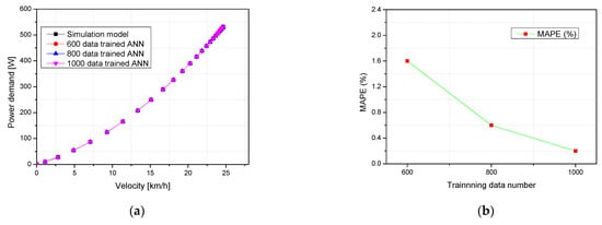
Figure 7.
(a) Comparison instructed with 600, 800, 1000 data point using one power-velocity curve, (b) comparison MAPE with 600, 800, 1000 data point.
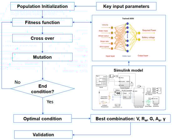
Figure 8.
The ANN-GA approach, informed by the Simulink simulation.
4. Results and Discussion
4.1. Validated Data
The experiments were carried out to provide basic ES performance data, which were validated with the simulation study. Figure 9 and Figure 10 show the comparison between the output data of the simulation and experiment. The straight lines describe the simulated results while the segmented line describes the experimental results. The rider mass was adjusted from 77 kg to 87 kg to evaluate the performance of the ES during moving conditions. Figure 9a presents the maximum difference of scooter velocity, which is 8.25% at 25 s. The scooter velocity is an experimental average value and is thus acceptable. When the wind speed, slope grade, wheel radius and ES mass are kept at a constant, the scooter velocity reduces with the increase in rider weight. Figure 9b–d show the validated moving distance and battery voltage. The same trend can be seen in the simulation and experimental values. The maximum difference in the moving distance and battery voltage are 3.53% at 56 s and 0.4% at 28.5 s, respectively.
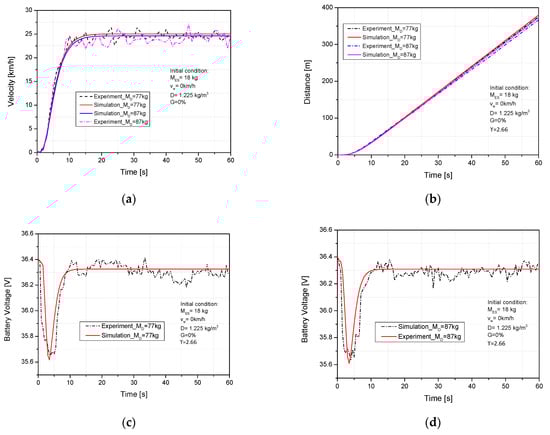
Figure 9.
(a) Velocity validation versus rider mass; (b) travel distance validation versus rider mass; and (c,d) battery voltage validation versus rider mass.
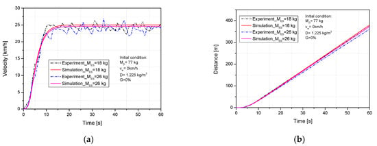
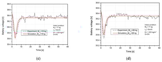
Figure 10.
(a) Velocity validation versus ES mass; (b) travel distance validation versus ES mass; and (c,d) battery voltage validation versus ES mass.
Figure 10 compares the simulation results and experiment results when the ES mass was varied. ES mass is an important factor in electric scooter specifications. It was chosen as an input parameter for validating the dynamic characteristics and battery voltage of the electric scooter. With an increase in ES mass, the velocity decreased from 25.04 to 24.62 km/h and the maximum difference was 9.42% at 45 s. Figure 10b–d shows that the moving distance decreased, and the electric consumption increased, when ES mass was increased. The moving distance and battery voltage correlated well with the experimental and simulated times. The maximum difference in the moving distance and battery voltage were 3.38% at 54 s and 0.47% at 47 s. After the validation, the steady simulated model supplied a corrected method to generate power demand and electricity consumption data. This will be used to forecast and enhance power demand and electricity consumption by combining the ANN and GA method.
4.2. Prediction of Power Demand and Electricity Consumption under the Influence of Structure and Operating Parameters
The paper thoroughly summarizes and discusses the key parameters affecting the dynamic and consumed energy of electric scooters during operating conditions, which have not yet been shown elsewhere in the literature. Therefore, the ANN model with one hidden layer and 12 neurons was incorporated with a GA optimization to predict and enhance power demand and battery voltage using wheel radius, slope ratio, scooter velocity, rider mass, and wind speed as input parameters. The parameters, each including 1000 data points from the simulation study, were used to train the ANN. Figure 11 shows the power demand and voltage versus scooter speed when changing the wheel radius. The dynamic and consumed energy during ES operation are sensitively influenced by the wheel radius. The ANN-GA approach was used in this work to forecast the optimal power demand and battery voltage output for five wheel radii, including 0.105, 0.125, 0.145, 0.165 and 0.185 m. As is illustrated in Figure 11a, the power demand increased from 534 W to 567 W when the wheel radius grew from 0.105 to 0.185 m. At 1.5 km/h and an Rw of 0.165 m, the largest discrepancy between the anticipated and simulated results is 4.5%. This could be explained by the fact that the increase in wheel diameter caused the scooter’s speed and inertia to increase. As a result, more power was needed to overcome the higher inertial force and reach the desired velocity. Figure 11b shows the battery voltage versus scooter velocity under five typical wheel radii. The wheel radius has a significant effect on battery voltage status during scooter operation; the voltage reduced from 34.48 V to 34.347 V during stable velocity behavior when the wheel radius grew from 0.105 to 0.185 m. The larger inertial force and velocity cause a rise in energy consumption. Because of this, when the wheel radius grows, the battery voltage falls to keep up with the higher energy demand.
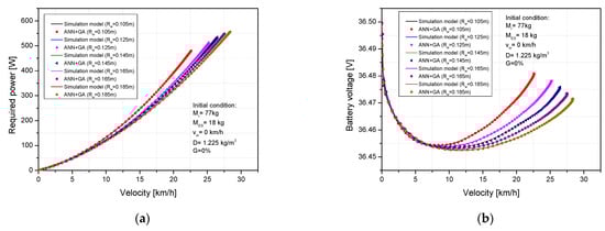
Figure 11.
Comparison between the simulated and ANN-GA predicted results of (a) power demand-velocity, (b) battery voltage-velocity curve under varying wheel radius.
Figure 12 presents the power demand and consumed energy versus the scooter velocity when the rider mass parameters were changed. Rider mass is one of the important operating factors in electric scooters, and has a significant impact on the power demand and electricity consumption. To examine the rider mass dependence on the optimized power demand and electricity consumption, the combined ANN-GA method was applied under five typical rider masses. As observed in Figure 12a, when the rider mass grew, the power demand showed an upward trend and a downward trend in scooter velocity, increasing from 497 to 521 W, and decreasing from 25.8 to 24.4 km/h, respectively. The maximum differences in the required power between forecasted and simulated results were 5.4% at 4.27 km/h with a rider mass sample of 57 kg. A lager rider mass will increase the inertial force while the other parameters are kept constant; therefore, the power demand will be greater to accommodate the increase in inertial force, namely, the rolling force. Figure 12b shows the influence of rider weight on battery voltage. Here, the rider mass grew from 57 to 97 kg; the battery voltage during stable scooter velocity showed a downward trend. This result is in agreement with the physical workings of the ES, which require more energy when the inertial force is greater, and the scooter is moving more slowly. This is also why the battery voltage dropped as the weight of rider rose.
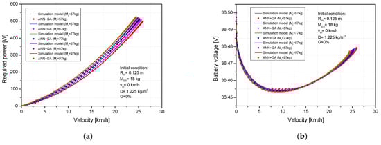
Figure 12.
Comparison between the simulated and ANN-GA predicted results of (a) power demand-velocity, (b) battery voltage-velocity curve under varying rider weight.
The slope grade has a sensitive influence to required power and battery voltage of ES during operation. As observed in Figure 13a the power demand increased when the slope grade rose. This is because the increase in required power was due to an increased slope resistance force, that will make a larger total resistance force. Therefore, the power to scooter overcome will be greater. As a result, when the slope grade rose from 0% to 1.15%, the demanded power rose from 510.2 to 554.3 W and the highest velocity dropped from 25.1 to 20.4 km/h, beside that, the highest difference between simulated results and predicted results was 4.2% at 2.4 km/h with slope grade of 1.15%. Figure 13b presents the effect of slope grade on battery voltage. It is evident that as the slope grade increases, the battery voltage lowers. This is also congruent with the basic principles behind ES operation: as the slope resistance force increases, so does the energy consumption. This explains why the voltage of battery decreased 0.02% when slope grade rose from 0% to 1.15%.
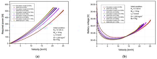
Figure 13.
Comparison between the simulated and ANN-GA predicted results of: (a) power demand–velocity; and (b) battery voltage–velocity curve under varying slope ratios.
When using a scooter, wind speed is a factor that is difficult to avoid and has a significant effect on scooter dynamics because the wind speed changing will directly affect to total resistance force of electric scooter during operation process. Here, the effect of wind speed on the required power is presented. As shown in Figure 14a, when the wind speed increases, the scooter velocity shows a downward trend and the required power shows an upward trend. The required power increases from 511.5 to 541.6 W when the wind speed increases from 0 to 4 km/h. The maximum difference between the simulated and predicted results is 6.6% at 12.7 km/h with a wind speed of 3 km/h. A larger wind speed will increase the wind resistance force while the other parameters remain constant; this will create a larger power demand for the scooter to overcome resistance force. This explains why the required power of scooter increases with increases in wind speed. According to Figure 14b, the battery voltage drops by 0.016% when the wind speed rises from 0 to 4 km/h. This results from the fact that an increase in wind velocity causes an increase in wind resistance force, which causes a higher energy requirement to accommodate a growth in the overall resistance force. Because of this, the battery voltage drops as the wind speed rises.
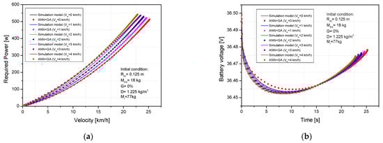
Figure 14.
Comparison between the simulated and ANN-GA predicted results of: (a) power demand–velocity; and (b) battery voltage–velocity curve under varying wind velocities.
The genetic algorithm (GA) optimization method was merged with a trained artificial neural network (ANN) model, with the ANN acting as the fitness function. The input factors for this enhancement included the wheel radius, rider mass, slope grade, wind speed, and scooter velocity. The output factors were the power demand and voltage. The ANN-GA method showed that the electric scooter could achieve an efficient performance range, with an optimized required power of 553 W and a maximum velocity of 28.2 km/h under a wheel radius of 0.185 m, a slope grade of 0% and a wind speed of 0 km/h. To validate the effective performance range and identify the associated input factors, the ANN-GA approach was used to forecast and optimize power demand under five typical scenarios for: wheel radius (0.105, 0.125, 0.145, 0.165, 0.185 m), rider mass (57, 67, 77, 87, 97 kg), slope ratios (0, 0.52, 0.79, 0.96, 1.15%), and wind speeds (0, 1, 2, 3, 4 km/h). The improved power demand and scooter velocity factors obtained by using the ANN-GA method are illustrated in Figure 15. The relationship between the optimized required power and slope grade can be seen in Figure 15a, where it is evident that the improved power demand rises as the slope ratio increases from 0% to 1.15%. This observation aligns with the physical principles governing scooter dynamics. As the slope grade increases, the scooter’s motion slows down, resulting in an increase in the required power. This is due to the fact that an increase in slope grade leads to a rise in both the slope resistance force and the total resistance force experienced by the scooter. In Figure 15b, it can be observed that the highest optimized power demand is 553 W, which occurs at a wheel radius of 0.185 m. Interestingly, this wheel radius also corresponds to the highest achievable velocity for the electric scooter within the range of wheel radii tested (0.105–0.185 m). As depicted in Figure 15c, the optimized power demand rises with an increase in wind speed. This observation aligns with the kinetic principles governing the operation of an electric scooter. When the wind speed rises within the range of 0–4 km/h, the scooter’s velocity decreases. This reduction in velocity is attributed to the higher wind resistance force. Consequently, the total resistance force experienced by the scooter increases, resulting in an increase in the required power. In Figure 15d, it can be seen that the optimized power demand rises, and the scooter velocity decreases, as the rider weight increases from 57 kg to 97 kg. This observation is in accordance with the physical principles governing the operation of electric scooters. With an increase in rider mass, the inertial force becomes larger, resulting in a greater total resistance power. Consequently, a higher required power is necessary to overcome the increased resistance and maintain the desired velocity. The findings of this study demonstrate that the forecasted results accurately reflect the significant physical motion and dynamic kinetics that impact the optimized power demand of electric scooters. The results show that the new ANN-GA method is an effective tool for determining optimized power demand and identifying the key input factors associated with it.
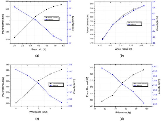
Figure 15.
The ANN-GA identifited four input factors that yields maximum power demand and veloicty: (a) five slope ratio, (b) five wheel radius, (c) five wind velocity, (d) five rider weight.
5. Conclusions
The proposed method with a combined ANN-GA approach was applied to forecast the power demand battery voltage, and to identify an effective performance range for an electric scooter. Each of the investigated parameters, obtained from a MATLAB-Simulink model, contained a total of 1000 data points and were applied for training, validation, and testing. One hidden-layer ANN structure with 12 neurons was applied with the slope ratio, rider mass, scooter velocity, wheel radius, wind speed as input parameters and the power demand and voltage as output parameters. Additionally, the GA was used to find the effective performance after the ANN had been trained. The ANN-GA approach was used to improve the effective performance of the electric scooter and its accompanying construction and operating parameters. The results showed that the electric scooter can attain 28.2 km/h with an optimum power demand of 553 W at a wind velocity of 0 km/h, a wheel diameter of 0.37 m, and a slope ratio of 0%. Furthermore, the forecasted results were correlated with the simulated results with an R2 value of 0.998. This demonstrated that the ANN-GA approach is an effective approach to solving complex problems, such as the performance prediction, identification, and operating control, of electric scooters.
Energy management systems for electric scooters are a promising research direction. In the future, an adaptive motor control system will be combined with the ANN method to consider the scooter’s current speed, acceleration, and load in order to adjust the power supplied to the motor. This will not only enhance the scooter’s performance but also ensure that energy is used judiciously, improving the scooter’s overall energy efficiency.
Author Contributions
L.T.H.: conceptualization, methodology, investigation, writing—reviewing formal analysis and resources; and editing. O.T.L.: supervision, and project administration. All authors have read and agreed to the published version of the manuscript.
Funding
This work was supported by Regional Innovation Cluster Development (R&D) by the Ministry of Trade, Industry and Energy (MOTIE, Korea) [Project Name: Open Innovation Project for Convergence Industry of Battery/Fuel Cell for Mobility Electrification and Energy Production/Storage (P0025406)]. This results was supported by “Regional Innovation Strategy (RIS)” through the National Research Foundation of Korea(NRF) funded by the Ministry of Education(MOE)(2021RIS-003).
Data Availability Statement
Data is contained within the article.
Conflicts of Interest
The authors declare no conflicts of interest.
Nomenclature
| Abbreviation | |
| ANN | Artificial neural network |
| ES | Electric scooter |
| GA | Genetic algorithm |
| LIB | Lithium-ion battery |
| NOx | Nitrogen oxides |
| HC | hydrocarbons |
| CO2 | Carbon dioxide |
| CO | Carbon monoxide |
| PV | Photovoltaic |
| MSE | Mean square error |
| ECU | Electric control unit |
| LM | Levenberg-Marquardt |
| PC | Slope resistance force, N |
| Latin symbols | |
| Aa | Frontal area, m2 |
| Rw | Wheel radius, m |
| Ca | Coefficient of aerodynamic drag |
| Crr | Colling coefficient |
| Cs | Slope coefficient |
| Tpf | Propulsion torque, N |
| Tm | Moment motor, N.m |
| M | Scooter and rider mass, Kg |
| Fpf | Propulsion force, N |
| Frrf | Rolling resistance force, N |
| Fsrf | Slope resistance force, N |
| Fwrf | Wind resistance force, N |
| La | Armature inductance, H |
| Ec | The back emf |
| Ra | Armature resistance, ohm |
| ia | Armature current, A |
| Ua | Terminal voltage of motor, V |
| Tl | Load torque, N.m |
| Te | Electromechanical torque, N.m |
| Ta | Acceleration torque, N.m |
| J | Inertia torque, N.m |
| B1 | Viscous friction coefficient |
| wm | Motor speed, rpm |
| Kb | Torque constant, N.m |
| Total power of battery, W | |
| Total power to propel vehicle, W | |
| Power loss by internal resitance, W | |
| Total resistive power, W | |
| Loss in power transmission | |
| Current of battery, A | |
| Open circuit voltage, V | |
| Battery available energy | |
| Terminal voltage. V | |
| Pfriction | Friction power, W |
| Pgrade | Slope grade power, W |
| Pwind | Wind power |
| t | Time, s |
| b | Bias value of neuron |
| xi | Input value if neuron |
| wi | Linked weight of neuron |
| p | The number of inputs |
| Greek symbols | |
| α | Slope ratio |
| Air density, kg/m3 | |
References
- Röck, M.; Saade, M.R.M.; Balouktsi, M.; Rasmussen, F.N.; Birgisdottir, H.; Frischknecht, R.; Habert, G.; Lützkendorf, T.; Passer, A. Embodied GHG emissions of buildings—The hidden challenge for effective climate change mitigation. Appl. Energy 2020, 258, 114107. [Google Scholar] [CrossRef]
- Ylä-Anttila, T.; Gronow, A.; Stoddart, M.C.J.; Broadbent, J.; Schneider, V.; Tindall, D.B. Climate change policy networks: Why and how to compare them across countries. Energy Res. Soc. Sci. 2018, 45, 258–265. [Google Scholar] [CrossRef]
- Shafique, M.; Azam, A.; Rafiq, M.; Luo, X. Life cycle assessment of electric vehicles and internal combustion engine vehicles: A case study of Hong Kong. Res. Transp. Econ. 2022, 92, 101112. [Google Scholar] [CrossRef]
- Breuer, J.L.; Samsun, R.C.; Stolten, D.; Peters, R. How to reduce the greenhouse gas emissions and air pollution caused by light and heavy duty vehicles with battery-electric, fuel cell-electric and catenary trucks. Environ. Int. 2021, 152, 106474. [Google Scholar] [CrossRef] [PubMed]
- Tutak, M.; Brodny, J. Analysis of the level of energy security in the three seas initiative countries. Appl. Energy 2022, 311, 118649. [Google Scholar] [CrossRef]
- Kamyk, J.; Kot-Niewiadomska, A.; Galos, K. The criticality of crude oil for energy security: A case of Poland. Energy 2021, 220, 119707. [Google Scholar] [CrossRef]
- Foissaud, N.; Gioldasis, C.; Tamura, S.; Christoforou, Z.; Farhi, N. Free-floating e-scooter usage in urban areas: A spatiotemporal analysis. J. Transp. Geogr. 2022, 100, 103335. [Google Scholar] [CrossRef]
- Stefan, G. Integrating e-scooters in urban transportation: Problems, policies, and the prospect of system change. Transp. Res. Part D Transp. Environ. 2020, 79, 102230. [Google Scholar]
- Lee, M.; Chow, J.Y.J.; Yoon, G.; He, B.Y. Forecasting e-scooter substitution of direct and access trips by mode and distance. Transp. Res. Part D Transp. Environ. 2021, 96, 102892. [Google Scholar] [CrossRef]
- Rehborn, H.; Koller, M.; Kaufmann, S. Data-Driven Traffic Engineering: Understanding of Traffic and Applications Based on Three-Phase Traffic Theory; Elsevier: Amsterdam, The Netherlands, 2020. [Google Scholar]
- Hichem, C.; Abdelfatah, N.; Kayisli, K. A Novel Method of Electric Scooter Torque Estimation Using the Space Vector Modulation Control. Int. J. Renew. Energy Dev. 2021, 10, 355–364. [Google Scholar] [CrossRef]
- Yuniarto, M.N.; Wiratno, S.E.; Nugraha, Y.U.; Sidharta, I.; Nasruddin, A. Modeling, Simulation, and Validation of An Electric Scooter Energy Consumption Model: A Case Study of Indonesian Electric Scooter. IEEE Access 2022, 10, 48510–48522. [Google Scholar] [CrossRef]
- Garman, C.M.; Como, S.G.; Campbell, I.C.; Wishart, J.; O’Brien, K.; McLean, S. Micro-Mobility Vehicle Dynamics and Rider Kinematics during Electric Scooter Riding; SAE Technical Paper 2020-01-0935; SAE International: Warrendale, PA, USA, 2020. [Google Scholar]
- Hu, J.-S.; Lu, F.; Zhu, C.; Cheng, C.-Y.; Chen, S.-L.; Ren, T.-J.; Mi, C.C. Hybrid Energy Storage System of an Electric Scooter Based on Wireless Power Transfer. IEEE Trans. Ind. Inform. 2018, 14, 4169–4178. [Google Scholar] [CrossRef]
- Di Giorgio, P.; Di Ilio, G.; Jannelli, E.; Conte, F.V. Numerical analysis of an energy storage system based on a metal hydride hydrogen tank and a lithium-ion battery pack for a plug-in fuel cell electric scooter. Int. J. Hydrogen Energy 2023, 48, 3552–3565. [Google Scholar] [CrossRef]
- Zhu, R.; Kondor, D.; Cheng, C.; Zhang, X.; Santi, P.; Wong, M.S.; Ratti, C. Solar photovoltaic generation for charging shared electric scooters. Appl. Energy 2022, 313, 118728. [Google Scholar] [CrossRef]
- Martínez-Navarro, A.; Cloquell-Ballester, V.-A.; Segui-Chilet, S. Photovoltaic Electric Scooter Charger Dock for the Development of Sustainable Mobility in Urban Environments. IEEE Access 2020, 8, 169486–169495. [Google Scholar] [CrossRef]
- Issi, F.; Kaplan, O. Simulation of a Wireless Charging Multiple E-Scooters using PV Array with Class-E Inverter Fed by PI Controlled Boost Converter for Constant Output Voltage. In Proceedings of the 10th International Conference on Smart Grid 2022, Istanbul, Turkey, 27–29 June 2022; pp. 61–65. [Google Scholar]
- Doubabi, H.; Oublaid, Y.; Salhi, I.; Chennani, M.; Essounbouli, N. A Reliable Power Management Strategy of a PV-Based Electric Scooters Charging Station. In Proceedings of the 7th International Conference on Optimization and Applications 2021, Wolfenbüttel, Germany, 19–20 May 2021; pp. 1–6. [Google Scholar]
- Hieu, L.T.; Khoa, N.X.; Lim, O.T. An investigation on the effective performance area of the electric bicycle with variable key input parameters. J. Clean. Prod. 2021, 321, 128862. [Google Scholar] [CrossRef]
- Hieu, L.T.; Lim, O.T. Effects of the Structure and Operating Parameters on the Performance of an Electric Scooter. Sustainability 2023, 15, 8976. [Google Scholar] [CrossRef]
- Hieu, L.T.; Khoa, N.X.; Lim, O.T. An Investigation on the Effects of Input Parameters on the Dynamic and Electric Consumption of Electric Motorcycles. Sustainability 2021, 13, 7285. [Google Scholar] [CrossRef]
- Channapattana, S.V.; Pawar, A.A.; Kamble, P.G. Optimisation of operating parameters of DI-CI engine fueled with second generation Bio-fuel and development of ANN based prediction model. Appl. Energy 2017, 187, 84–95. [Google Scholar] [CrossRef]
- Pai, P.S.; Rao, B.S. Artificial Neural Network based prediction of performance and emission characteristics of a variable compression ratio CI engine using WCO as a biodiesel at different injection timings. Appl. Energy 2011, 88, 2344–2354. [Google Scholar]
- Liu, X.; Fotouhi, A. Formula-E race strategy development using artificial neural networks and Monte Carlo tree search. Neural Comput. Appl. 2020, 32, 15191–15207. [Google Scholar] [CrossRef]
- Seo, J.; Park, S. Optimizing model parameters of artificial neural networks to predict vehicle emissions. Atmos. Environ. 2023, 294, 119508. [Google Scholar] [CrossRef]
- Yang, R.; Yan, Y.; Sun, X.; Wang, Q.; Zhang, Y.; Fu, J.; Liu, Z. An Artificial Neural Network Model to Predict Efficiency and Emissions of a Gasoline Engine. Processes 2022, 10, 204. [Google Scholar] [CrossRef]
- Carr, J. An introduction to genetic algorithms. Sr. Proj. 2014, 1, 7. [Google Scholar]
- Hieu, L.T.; Lim, O.T. A deep learning approach for optimize dynamic and required power in electric assisted bicycle under a structure and operating parameters. Appl. Energy 2023, 347, 121457. [Google Scholar] [CrossRef]
Disclaimer/Publisher’s Note: The statements, opinions and data contained in all publications are solely those of the individual author(s) and contributor(s) and not of MDPI and/or the editor(s). MDPI and/or the editor(s) disclaim responsibility for any injury to people or property resulting from any ideas, methods, instructions or products referred to in the content. |
© 2024 by the authors. Licensee MDPI, Basel, Switzerland. This article is an open access article distributed under the terms and conditions of the Creative Commons Attribution (CC BY) license (https://creativecommons.org/licenses/by/4.0/).