Abstract
Stability-dependent far-field offshore wind-farm wakes are detected in Supervisory Control and Data Acquisition (SCADA) wind power records from wind farms located in the North Sea. The results are used to assess the strengths and weaknesses of the Openwind engineering model, which in turn enables understanding of the wake signal captured by the SCADA data. Two experimental model set-ups are evaluated, the current standard set-up considering a neutral atmosphere and extended for stable conditions, and the other using a new atmospheric stability implementation called the far-wake atmospheric stability model (ASM) previously reported in Energies. The ASM approach enables the identification within wind power records of wakes of length at least 30 km depending on the atmospheric stability. The ASM approach would be useful for assessing which neighboring wind farms are likely to affect the wind turbine power output and to what extent the power output is affected by stability.
1. Introduction
Flow modifications due to a single or a few offshore turbines in a group as found in the earliest demonstration wind farms, such as alpha ventus in the North Sea [1], pale in complexity compared with the long-range effects on the freestream flow due to whole clusters of wind farms grouped together [2]. The integrated effect of wakes from individual turbines, individual wind farms, or clusters of wind farms grouped together, on the overall flow situation up to the mesoscale ( km) [3] is of particular interest to, among others, current and prospective wind farm operators and investors, because wakes equate to losses and inefficiencies [4]. The challenge faced by modellers in providing insight into these phenomena is how to quantify the cumulative effects of various flow and wake inefficiencies (e.g., surface roughness [5], wind turbine induction [6], turbine wakes [7], wind-farm flow [8], wind-farm wakes [9], cluster wakes [10]) of different scale on the expected wind farm energy yield, and which atmospheric parameters need most be considered in their assessments [11]. Some of the commonly used tools for making such energy yield assessments are Openwind [12], Windfarmer [13], and WAsP [14].
Energy yield assessment is essentially the task of estimating the expected wind energy output of a wind farm given a freestream wind speed climate while accounting for any important flow losses, such as wind turbine wakes [15]. The wind speed reduction in the wake of a single wind turbine can be simply modelled with one of the classic analytical wake models proposed some 40 years ago by Jensen [16] or Ainslie [17], or more recent popular ones such as that proposed by Bastankhah and Porté-Agel [18] or the TurboPark model [19]. These tools are some of the more traditional and still standard ways of accounting for the wind turbine wakes within wind farms in energy yield assessments [3]. The added complexity on the flow itself due to arrays of wind turbines grouped together has been addressed many years ago by Frandsen [20], Emeis and Frandsen [21]. The ‘Frandsen approach’ is to consider wind farms as an added source of roughness [22] resulting in the growth of an internal boundary layer above, and a modified wind speed profile within, the wind farm based on the ground and added-turbine surface roughnesses [23]. The modified wind-farm wind speed profile can be blended with one of the aforementioned turbine wake models to build a coupled wind-turbine–farm wind speed model, such as that calculated by the combined eddy viscosity–deep-array wake model (DAWM) available in Openwind [24]. Despite the many [3,11] advances in wake modelling, for industry, this is, more or less, the state of the art [25].
The Frandsen approach has been extended to consider the effect of atmospheric stability on the wind-farm wind speed profiles [26,27] by invoking Monin–Obkuhov similarity theory. Atmospheric stability acts to dampen the vertical exchange of momentum between the wake and freestream flow, resulting in a slower wind speed recovery downstream for wakes in stable conditions; an equivalent process occurs if the surface roughness is lower [28]. Atmospheric stability is an important consideration in regions where clusters of wind farms are present, such as in offshore environments, since stable conditions can persist for days, and the surface water roughness is orders of magnitude lower than over land [29]. Thus, Emeis et al. [30] extended the Frandsen approach to consider the stability-dependent wind-speed recovery many kilometres downstream with a view to optimizing the wind farm layout based on the stability climate at the intended site [31]. Is the extra computational effort and physical uncertainty of including stability worth deploying in engineering models like Openwind?
Much modelling work has been invested in demonstrating the importance of long wakes from offshore wind farms [32,33], particularly in stable conditions [34] which probably extend many tens of kilometres downstream. Measurements of hub wind speed using a number of different techniques such as with lidar [10], aircraft [35], and satellite observations [36] have demonstrated the stability dependence of far wakes on offshore flow [37], but to what extent can we see these effects in the wind power measurements of turbines? From the perspective of an operator, the satellite images and modelling studies of long wakes may be merely interesting until hard and persistent evidence of an effect on turbine power can be demonstrated. From the perspective of a modeller, wind farm designer, or energy yield assessor, increasing the number of wind farms needed to be considered in simulations will increase the computational complexity of the problem. Hence, some guidance as to the size of the modelling domain or the number of neighbouring wind farms to be included in investigations is needed.
In the following, we report on the extent to which stability-dependent far-wake effects evident in SCADA wind power records are able to be depicted in a conventional engineering model. The SCADA wind power data are sourced from a number of wind farms in the North Sea and the Openwind model is used because we are most familiar with it and for its ability to represent the long-range stability effects of wakes quickly and relatively realistically [37]. The scale of wakes is increased sequentially, beginning with the stability dependence of internal wakes, then near wind-farm wakes which we define as those < (10 km), followed by far wakes (10 km), and ending with some speculations regarding very long wakes up to (100 km). Demonstration that the measured qualitative shape of wakes and their quantitative dependence on stability are equivalent to engineering modelling results gives further evidence and confidence in the importance of this phenomenon in assessments of the overall energy gains expected from clusters of offshore wind farms.
2. Methodology for Far-Wake Quantification Using SCADA Data
With the help of flow modelling and the wind-farm performance as determined from the wind turbine SCADA systems, the arrangement of certain wind farms in the North Sea enables the simultaneous analysis of wake effects at the wind turbine level up to the scale of wind farm clusters. Those wind farms considered are described in this section together with the post-processing of SCADA data from these farms.
2.1. Wind Farm Details
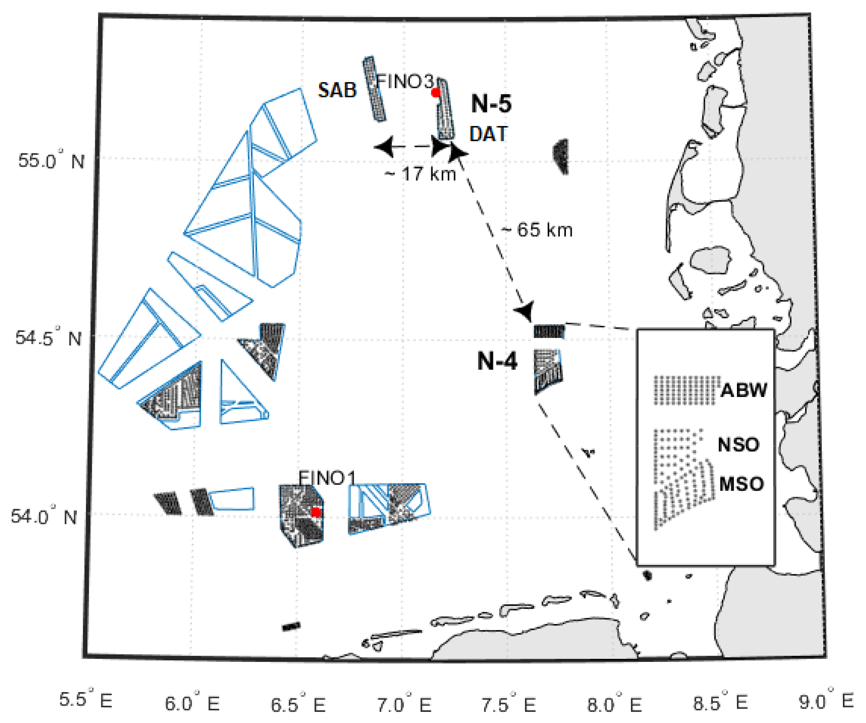
Our analysis is centred on the Amrumbank West (ABW), Nordsee Ost (NSO), Meerwind Süd|Ost (MSO), DanTysk (DAT), and Sandbank (SAB) wind farms located in the North Sea as sketched in Figure 1. The ABW, NSO, and MSO wind farms comprise the N-4 cluster, which includes the recently built Kaskasi wind farm, but here is called the ‘Kaskasi Gap’ because it is missing for the period of data considered. The Kaskasi Gap is located between the ABW and NSO wind farms, which are separated in the north–south direction by about 4 km. About 65 km to the north-north-west are the DAT and SAB wind farms that comprise the N-5 cluster, and these farms are separated by a east–west gap of 17 km.

Figure 1.
Map of the North Sea area showing the locations of the Sandbank (SAB) and DanTysk (DAT) wind farms (N-5 cluster) with respect to the Amrumbank West (ABW), Nordsee Ost (NSO), and Meerwind Süd|Ost (MSO) (N-4 cluster) wind farms including the measurement platforms FINO1 and FINO3 (red points) [38]. Also indicated are other existing (black points) and planned (blue borders) wind farms further west as of 2022 in the German sector of the North Sea.
Table 1 presents some of the basic technical details of the wind farms. Figure 1 shows that the ABW wind farm is a classic regularly spaced, near-symmetric wind farm, while the turbine arrangements of the NSO and MWS farms are more staggered. The DAT and SAB farms, with approximately regularly spaced east–west turbine rows consisting of 4–5 turbines, are more elongated in the north–south directions compared with the N-4 cluster farms. Due to the lack of SCADA data from the MSO wind farm, located directly south of the NSO wind farm, flow from the south cannot be taken into account due to the unknown inflow conditions. As the N-4 cluster lacks a meteorological mast for use in determining the input conditions, the upstream turbines of the ABW and NSO farms are used to define the reference conditions. The FINO3 mast east of the DAT wind farm could be used to help define the input conditions there, but it is in the far-wake of the western SAB wind farm for flow from the west, and the DAT farm for flow from the east. Therefore, undisturbed wind turbines are also used to define the inflow conditions of the N-5 cluster. As shown in Table 1, turbine data (10 min mean values of wind speed, nacelle position, power, pitch angles) are evaluated for the period 2015–2021 for the N-4 cluster and 2018–2020 for the N-5 cluster.

Table 1.
Basic properties of the turbines within the wind farms within the N-4 (ABW, NSO, MSO) and N-5 (DAT, SAB) clusters (SWT: Siemens wind turbine; Re: RePower).
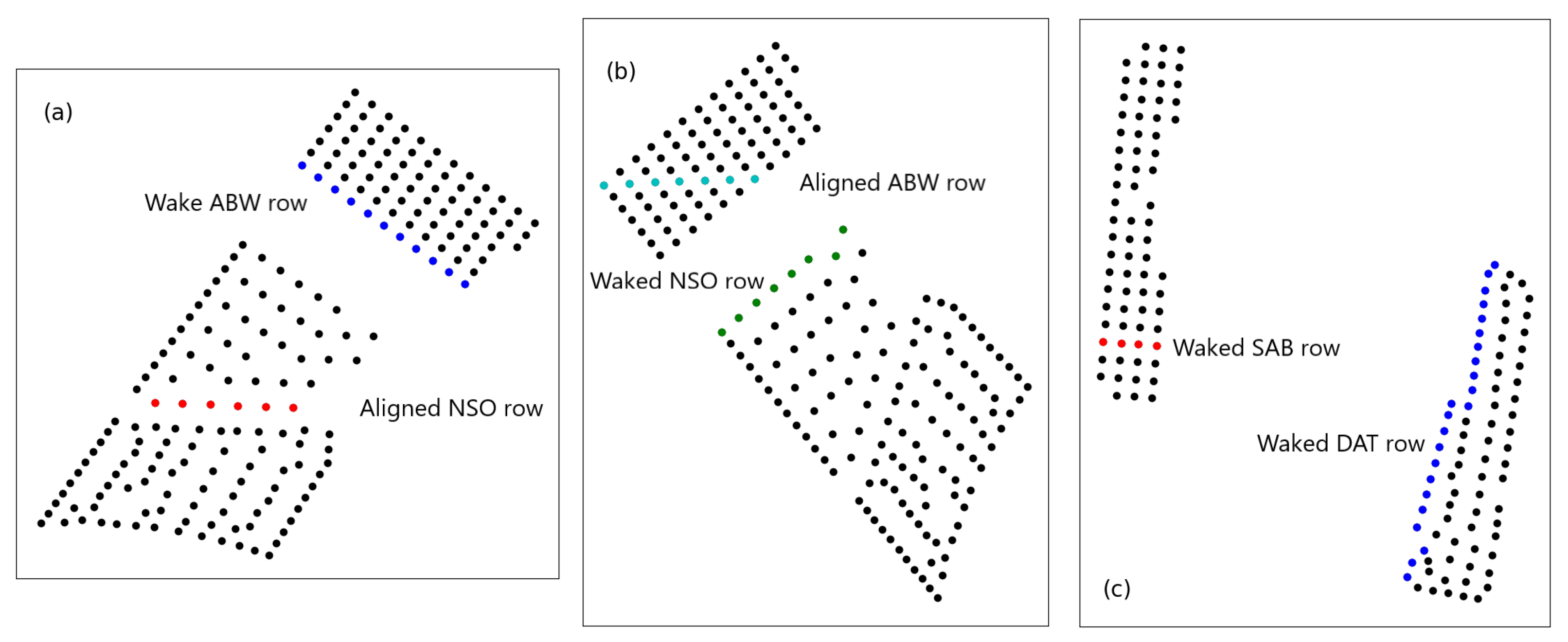
Figure 2 illustrates that certain orientations of the N-4 and N-5 clusters may be exploited to emphasize particular internal, near, and far-wake effects. For a south-westerly flow to the N-4 cluster, the southern ABW row is partially waked by the NSO farm, while there is an aligned row (canonical wake situation) within this farm as illustrated in Figure 2a (red points). For a north-westerly flow to the N-4 cluster, the northern NSO row is partially waked by the ABW farm, while at the same time one selected wake row of ABW as indicated in Figure 2b acts as an aligned canonical wake row. The N-5 cluster (Figure 2c) for different wind directions allows the tracking of the far-wake effects of the SAB wind farm on the front row of DanTysk, as well as some internal wakes, although for this orientation there are only four or five turbines in a row.
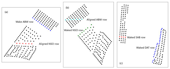
Figure 2.
Highlighted features of the N-4 cluster for south-west (a) and north-west (b) flows showing aligned wakes within the NSO (red) and ABW (cyan) wind farms and the directly waked “front rows” of the ABW (blue) and NSO (green) wind farms (black dots). Panel (c) shows the N-5 cluster for a western wind direction. The front row (blue) of the DAT wind farm is indicated as well as one of the aligned wake rows (red) of SAB for this wind direction.
2.2. SCADA Data Post-Processing
In any wake analysis, it is necessary to post-process SCADA data prior to use to account for the many periods of power reduction and downtime when the turbine is operating suboptimally for technical reasons unrelated to wake–turbine interactions.
The following basic filtering procedure of the SCADA data has been performed. Wind speeds and power less than 3.5 m/s and 0 kW, respectively, are automatically filtered. An initial “ideal” blade pitch angle region is defined to detect an ideal power curve, from which a moving mean is calculated—this is extrapolated down to wind speeds of 0 m/s and out to 25 m/s. Right and left bounds are defined using the curves proposed by Doekemeijer et al. [39] with reference to the initial estimated power curve based on the pitch angle. All records inside the bounding curves are included in the final dataset to be compared with the flow model output. Other errors also appear in the SCADA time series, such as short-term data drop-outs that have to be removed from consideration, while biases in the wind direction have been corrected following the method outlined in Doekemeijer et al. [39].
An example of the filtering procedure and resulting filtered data for a single turbine is shown in Figure 3. Evident are large numbers of power curtailments below the expected power curve approximated by the black points, including a roll-off of power at higher wind speeds. However, since the focus here is on far wakes, we are interested in the part of the power curve from approximately 6 to 10 m/s as shown by the red rectangle in Figure 3. We have not attempted to correct the wind speeds and thus are relying on the accuracy of the operators’ calibrations.
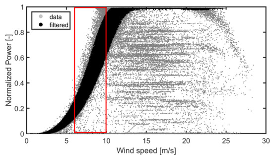
Figure 3.
An example of the filtering procedure for the SCADA data from a single turbine showing first all possible data for the time period (grey) and then the filtered data (black) to be used for analysis. The red rectangle indicates the region of the power curve considered here.
Offsets in the nacelle’s direction have been determined using the energy ratio R as part of the FLASC tool described by Doekemeijer et al. [39]. We also use the energy ratio R in our analysis below but interpreted purely as a ratio of summed 10 min power values, where
to quantify the power production p [kW] of a particular wind turbine with respect to some reference ( [kW]) turbine least affected by wakes. In the calculation of R, each stability and wind direction bin is determined in the following way. The wind direction bin sizes are fixed at 15. Nominal wind speed bins are initially set to include data in the partial load part of the power curve 6–10 m/s as indicated by the red rectangle in Figure 3 where wake effects are expected to be maximum. This range may vary to ensure approximate mean wind speeds of 8 m/s for all bins. Nominal stability bins are also used and then adjusted to ensure mean values of , 0.5 and 1.5, which are the stability classes used in the analysis below. As wind speeds increase above 10 m/s, which is roughly just below the rated power of a wind turbine, wake effects become less obvious before disappearing at even higher wind speeds where they are generally ignored. Moreover, very stable atmospheric conditions become less frequent above the rated wind speed before disappearing completely at even high wind speeds [40]. The selection of a wind-direction bin width of 15 is a trade-off between the number of points selected and capturing the wind-direction-dependent phenomenon. A large bin width smooths the direction-dependent effects, while a small bin width allows more scatter into the curves. We neglect horizontal inhomogeneity as a first-order approximation, but at larger scales, the wind direction may vary by about 10 at the wind speeds considered here [41]. We have set the minimum number of data points for each bin to be 11.
Additionally, we filter data for stability in terms of the Monin–Obukhov stability parameter, where the Obukhov length
calculated from the surface-layer parameterization of the Weather Research and Forecasting (WRF) model for a grid point located close to the N-4 cluster and at FINO3 for use at the N-5 cluster. Here, is the friction velocity, is the von Karman constant, g is the acceleration due to gravity, is the potential temperature, and is the kinematic heat flux. Version 4.2.1 of the WRF model was used, with three domains of 18, 6, and 2 km resolution all centered over the German clusters of wind farms in the southern North Sea. Boundary-layer turbulence was accounted for with the Mellor–Yamada–Nakanishi–Niino (MYNN) parameterization, and 6-hourly ERA5 data were used as model input. Further details of the WRF set-up, including the positions of the three domains, can be found in Section 2.2 of Cañadillas et al. [10].
For example, if we wish to calculate the energy ratio of some turbine with respect to the reference turbine, we sum all power within the wind speed, wind direction, and stability range of both the turbine of interest and the reference turbine and calculate R therefrom. Note that if a missing value is detected in either the reference or turbine of interest, then this value is not included in the magnitude of R.
3. Flow Modelling with Openwind
The flow modelling part of this work is meant to assist in wake identification. In practice, we also wished to see to what extent far wakes are captured with Openwind. Openwind is a commercial wind farm flow simulation and energy yield analysis suite used by many industry users to, for example, prospect potential wind farms and analyze the energy outputs of existing ones. Since layout optimizations are performed requiring many simulations, both computational speed and model fidelity, are two aspects that are particularly emphasized in the Openwind software [12]. More detailed flow field investigations are typically reserved for more computationally demanding tools, such as large-eddy simulations, but for commercial applications, these are well beyond the current computing power.
For a typical time series energy capture, freestream wind speeds from, for example, a met mast, model, or undisturbed wind turbines, are used to drive the input wind speeds used in the calculation of the power output from a wind farm. In the absence of any wakes, the wind farm power can be derived simply from the turbine power curves as a function of wind speed for each of the wind turbines. Taking into account wakes requires the use of a wind turbine wake model, such as the Eddy Viscosity approach [17] or the TurboPark model [19] commonly used in Openwind, to modify the wind speed and turbulence downstream from each of the wind turbines. Induction, which is the deceleration of the upstream wind speed, has also recently been included in Openwind [42,43,44], which can reduce the wind farm power by a few per cent depending on the set-up [37]. Note that any model involved in the energy capture and wind-farm optimization process needs to be quick and accurate because thousands of different simulations may need to be performed in a relatively short period of time. Here we briefly describe two such approaches in Openwind for accounting for atmospheric stability, one more established called the Deep-Array Stability Model (DAWM), and the other more experimental called the Atmospheric Stability Model (ASM).
By grouping wind turbines together into wind farms, it is hypothesized that there is an added wind speed deficit exceeding that produced by wind turbine wake models alone. The DAWM approach [24] is used to account for groupings of wind turbines contributing to the progressively increasing energy deficit with increasing depth into the wind farm. The DAWM approach considers upstream wind turbines as an enhanced source of surface roughness (turbine roughness) that modifies the downstream wind speed profiles as seen by the wind turbines further into the wind farm. The maximum wind speed deficit resulting from the DAWM-modified wind speed profiles and turbine-waked wind speeds gives the reduced incoming wind speed to any downstream wind turbine.
Although not the default option which is for neutral conditions, atmospheric stability may be included in the DAWM approach in the calculation of the wind speed profiles due to the similarity theory of Monin and Obukhov [45], where the freestream wind speed at hub height
with the surface roughness length, the stability correction for varying , and the Obkuhov length L defined above in Equation (2). For the DAWM approach, Brower and Robinson [24] give an approximation for the ratio of the hub height wind speed within the wind farm due to an added turbine roughness that we modify here based on Equation (2) to give
In stable conditions, , (4) tells us that as becomes large, which implies the wind speed reduction in very stable conditions becomes negligible, which we suspect is unrealistic (see also Peña and Rathmann [27]). Alternatively, the ASM approach described in [37] is based on the far-wake wind speed recovery procedure presented in Emeis [46]. This approach is also derived from stability-dependent wind speed profiles defined according to Monin–Obukhov similarity theory. It does not include an added turbine roughness, but instead uses a stability-dependent mixing coefficient to account for the wind speed reduction within the wind farm and a stability-dependent exponential recovery function downstream of the wind farm (see Cañadillas et al. [35,37], for more details). In contrast to the DAWM approach, ASM is essentially a stability-dependent drag model also applicable to mesoscale parameterizations as demonstrated conceptually in Foreman et al. [29].
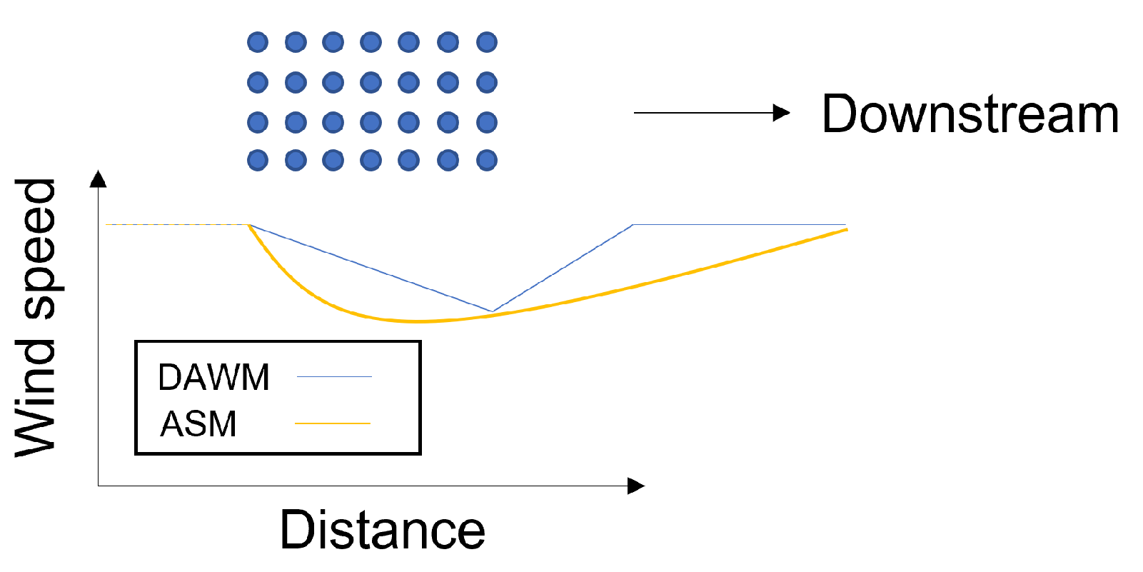
A conceptual comparison between the two approaches is sketched in Figure 4 and the basic set-up of each model is shown in Table 2 (see [37] for more details). For the DAWM approach, there is an increasing wind speed deficit deeper into the wind farm and then a relatively quicker recovery downstream. The tunable parameter for that model is the wind turbine roughness which is set to 1.16 m here. In contrast, the ASM wind speed deficit within the wind farm reflects the turbine density with a more gradual, exponential recovery downstream [35] depending on the atmospheric stability and the tunable parameter (here set to , where D is the turbine rotor diameter) described in Cañadillas et al. [37]. This parameter deviates from approximately the rotor diameter D depending on the interaction between the background boundary-layer flow and the layout of the wind farm. For a typical energy capture, such as one would perform for a wind farm in the N-4 cluster, the DAWM approach for offshore conditions together with the Eddy Viscosity model would usually be run using provided freestream wind conditions, but in practice without a stability dependence. For the assessment of longer wakes, the ASM approach may yield more realistic information about long wakes, such as the 20 km separation of the SAB and DAT wind farms in N-5.
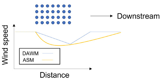
Figure 4.
Sketch comparing the relative wind speed deficit and recovery within and downstream from a wind speed (circles) between the DAWM and ASM approaches in Openwind.
Table 2.
Key parameters of the Openwind set-up and input parameters for each wake model for comparison with the SCADA data (L is the Obukhov length).
For comparison with power derived from SCADA data, outputs from the Openwind engineering suite are used as a reference to help interpret the SCADA wake analysis. For this purpose, Openwind has been run in time series mode for the same period of time defined by the SCADA data shown in Table 1.
A description of the energy capture methodology for both the DAWM and ASM approaches is provided in Section 2 of Cañadillas et al. [37] as well as references for Openwind. An internal developmental version of Openwind containing experimental models and parameterizations is used for simulations. The inputs to the model are an assumed freestream wind speed and direction estimated from the upstream wind turbines and the Obukhov length from the WRF model near the N-4 cluster and the WRF model at FINO3 for the N-5 cluster as mentioned above. The SCADA-derived wakes from the N-4 clusters are simulated with the stability-dependent DAWM approach, while the far wakes between the two wind farms of cluster N-5 are investigated with the help of the ASM approach.
4. Results
Results of the SCADA measurements are first presented for the N-4 cluster for the purpose of quantifying the stability dependence of internal wakes and the propagation of these wakes downstream in the near field. In this situation, a typical model set-up would be a wake model with a DAWM approach without stability effects included, but here we consider the atmospheric stability part of the DAWM approach with respect to the SCADA results. Far-field wake effects in the SCADA measurements are then investigated in the N-5 cluster with the help of the ASM approach in Openwind. A discussion proceeds the presentation of results where we briefly discuss the very far field situation of wakes from N-4 on N-5, which has also been modelled with the ASM approach.
4.1. N-4 Cluster Wakes for Flow from the West
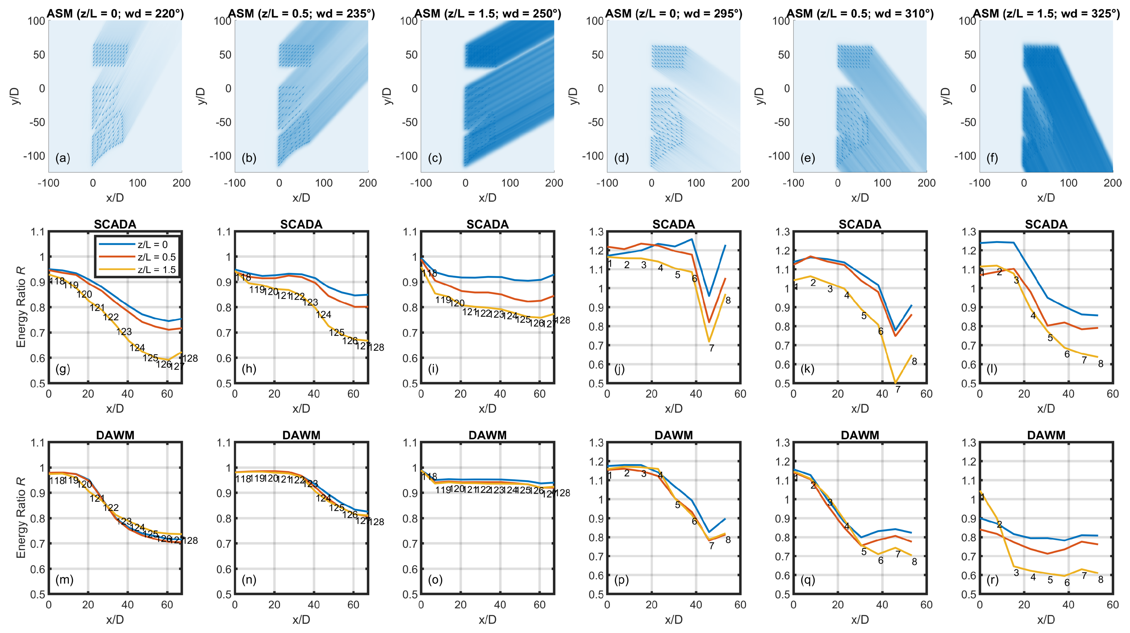
Figure 5a–f presents two-dimensional representations of the flow through the N-4 cluster at a freestream wind speed of 8 m/s according to the ASM approach for the wind directions of (a) 220, (b) 235, (c) 250, (d) 295, (e) 310, and (f) 325 for (a, d) neutral (), (b, e) stable (), and (c, f) strongly stable () conditions. The different wind directions illustrate the wake impacting the southern row of the ABW wind farm (a–c, turbines 118 to 128) and the northern row of the NSO wind farm (d–f, turbines 1 to 8). The different stability classes illustrate the increasing wind speed deficit with increasing stability according to the ASM approach. With increasing atmospheric stability, internal wakes tend to blend into the integrated wind farm flow as evident in the disappearance of lighter shades (freestream wind speed) within the wind farms for and 1.5. Figure 5a,d show that the neutral flow simulated by standard wind turbine wake models [in this case the eddy viscosity model] [17] would almost ignore the effect of the wake on the downstream wind farm, particularly in stable conditions. Figure 5g–l show the SCADA energy ratios at the southern ABW row (g–i) and northern NSO row (j–l) for , 0.5, and 1.5 at the wind directions 220, 235, 250, 295, 310, and 325, respectively. The numbers represent the positions of the turbines according to their labels shown below in Figure 6 and Figure 7. We will explain these figures before returning to the energy ratios shown in Figure 5.

Figure 5.
(a–f) Wind speeds according to the ASM approach for the wind directions (stability) 220 (), 235 (), 250 (), 295 (), 310 (), and 325 () for a freestream wind speed of 8 m/s. Corresponding normalized energy ratios R for these wind directions and stabilty classes according to the SCADA (g–l) and DAWM (m–r) approach. The numbers of the individual turbines correspond with the turbine numbers in Figure 6 and Figure 7 and represent their positions at along the curve . The left-hand three panels show the southern row of ABW and the right-hand three panels show the northern row of NSO.
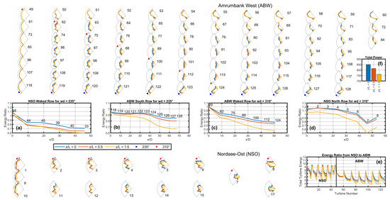
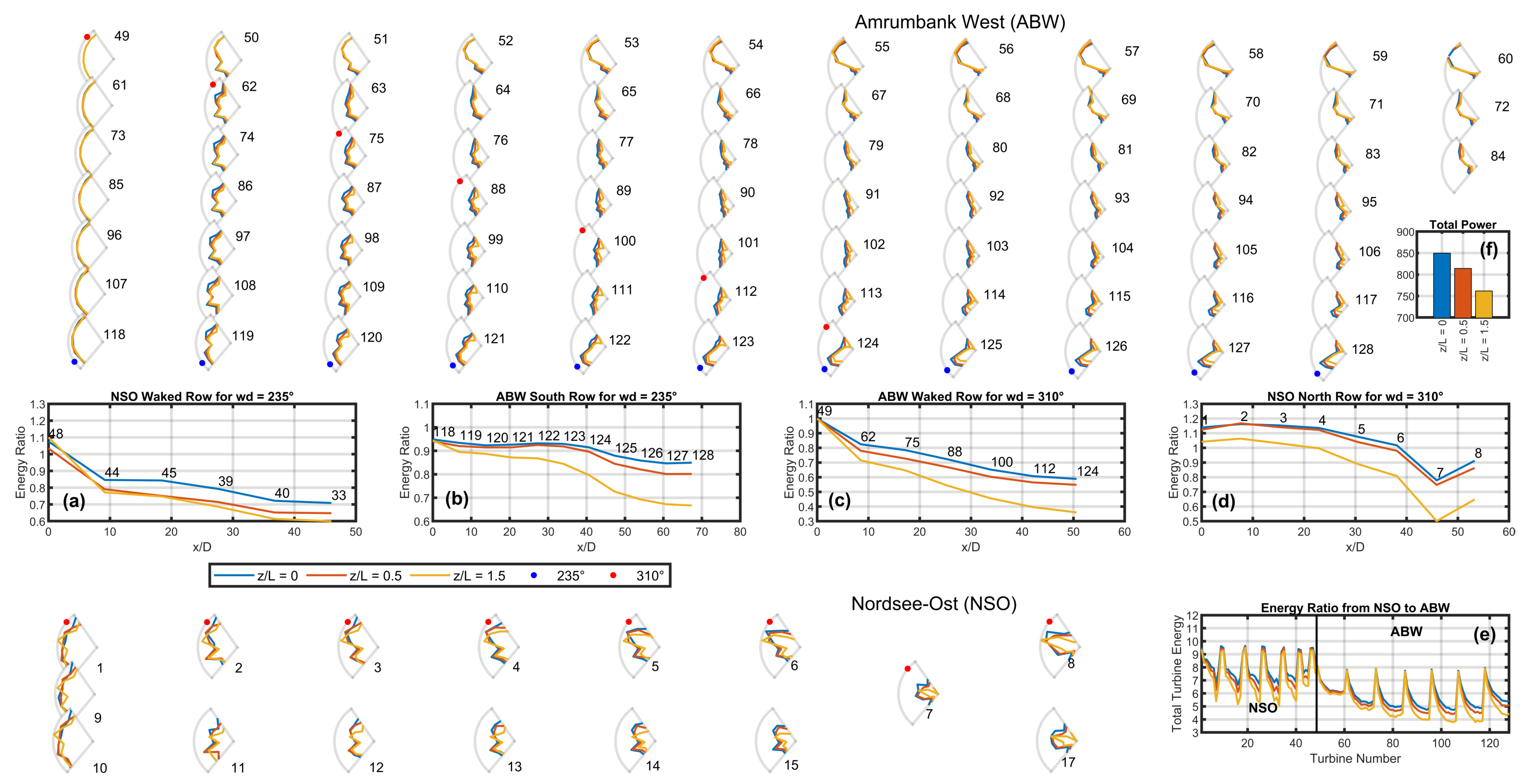
Figure 6.
Partial polar plots (220–325) of normalized SCADA energy ratio (with respect to turbine 49 located at the north-west of ABW) for wind turbines of the NSO and ABW wind farms for Monin–Obukhov stability parameters of 0 (blue), 0.5 (red), and 1.5 (yellow). Two particular wind directions involved in the subplots (blue: 235; red: 310) are highlighted as points on the corresponding polar plots. The polar plots are arranged at the relative positions of the wind turbines (their numbers indicated) within the ABW and NSO wind farms. Note only the first northernmost rows for the NSO farm are shown because of space constraints. Subplots show the energy ratio as a function of downstream distance (normalized to the corresponding first turbine in the series) for (a) the southernmost NSO row for a wind direction of 235 (to see this aligned row, refer to Figure 2b above), (b) the southernmost ABW row for a wind direction of 235 (blue points), (c) an internal ABW wake for a wind direction of 310 (red points in ABW), and (d) the northernmost NSO row for a wind direction of 310 (red points in NSO). The numbers within these subplots indicate the turbine positions along . The summed energy ratios (e) are shown for all turbines of the NSO and ABW wind farms, and the summed total energy (f) of the cluster (only ABW and NSO) for each stability class.
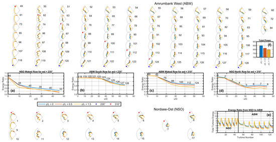
Figure 7.
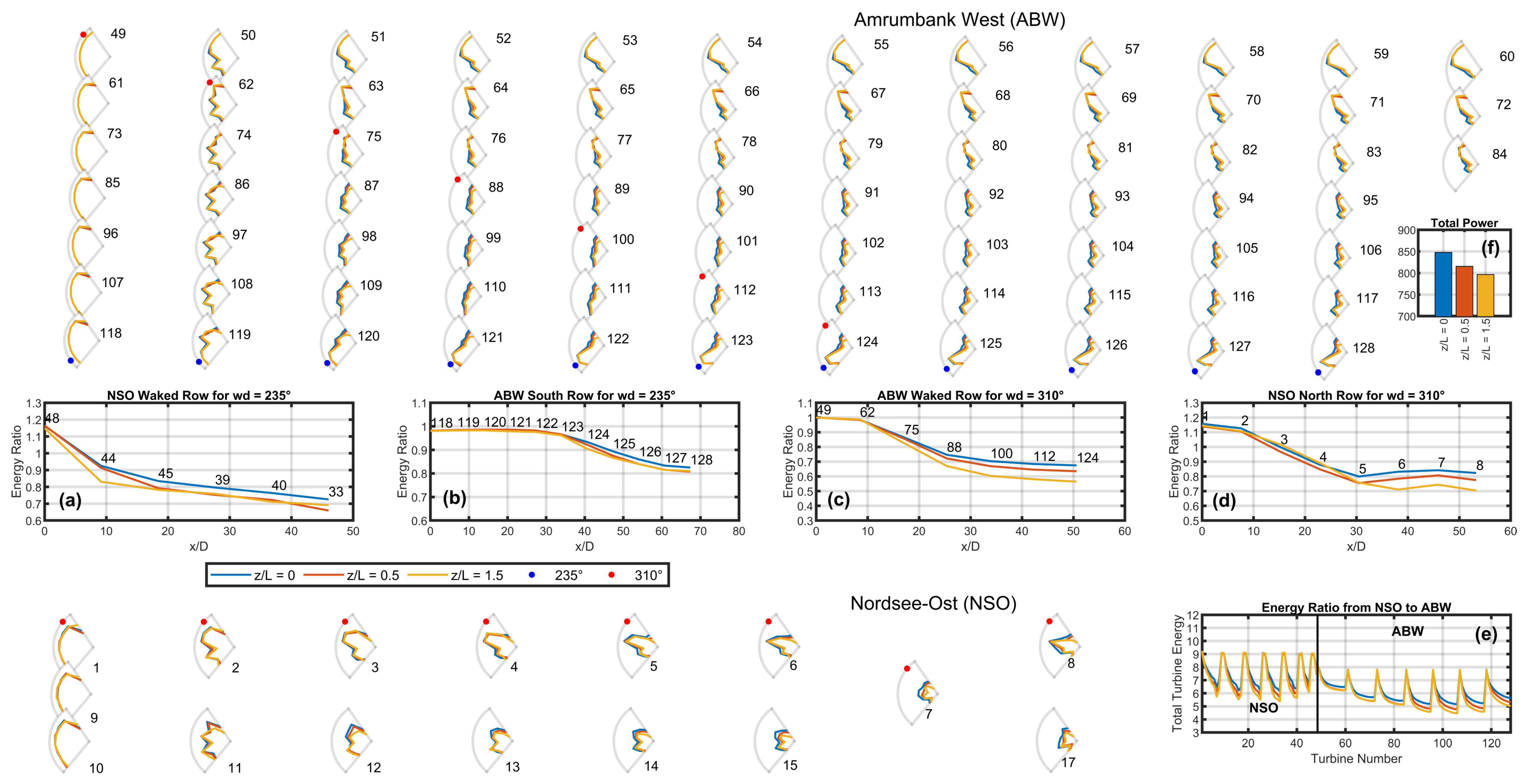
As Figure 6 but for the DAWM calculated energy ratios.
Figure 6 and Figure 7 present, respectively, SCADA and Openwind (DAWM) energy ratios R according to Equation (1) in the form of partial polar plots at the relative positions of the wind turbines for wind directions 220–340 for data grouped in 15 bin widths. Hence, seven points are presented in each polar plot for Monin–Obukhov stability parameters of (neutral, blue), 0.5 (stable, red), and 1.5 (strongly stable, yellow). All polar plots are normalized with respect to turbine 49, which is located at the north-west corner of the ABW farm, and thus the plot for turbine 49 is simply the arc of a unit circle from 220 to 340. Summing over all points of the polar plot of turbine 49 equates to a value of 7 (because it is normalized with itself), but for the waked turbines within the ABW farm and downstream from the freestream turbines, the summed energy ratio is less than 7. Along the top row of ABW turbines (see the plots labelled 49–60), there is an increasing distortion of the polar plots in the south-western direction further into the wind farm. Heading south within the ABW farm beginning at turbine 59 (along turbines 71, 83, 95, 106, 117, 128), there is an increasing distortion of the energy ratio deeper into the wind farm but then a slight recovery along the southern ABW row in the south-western direction, corresponding to the Kaskasi Gap separating the ABW and NSO farms.
The panels positioned between the ABW and NSO wind farms give more detailed snapshots of the energy ratio for selected rows (a–d) or the overall wind farm (e, f). For example, panel e shows the summed values of all turbines from 1 to 128, with turbine 49 at the vertical line separating the two farms giving a summed energy ratio . To the right of the vertical black line in (e) lie the ABW turbines (from 49 to 128), with the periodic peaks representing the westernmost column (turbines 61, 73, 85, 96, 107, 118) of the ABW farm in presumably freestream conditions for the westerly flows considered here. (Actually, there is a slight upstream blockage effect detected in this group of turbines). On the left side of panel e are turbines 1 to 48 representing the summed energy ratios for the NSO wind farm. Note that only polar plots for the first few northern rows of the NSO farm are displayed due to spatial constraints. The NSO peaks in panel e also represent the western row of the NSO farm in freestream conditions but reach higher values (=9.5), probably because of the more powerful NSO wind turbines (see the rated powers in Table 1) with respect to the ABW turbines.
Panels a–d in Figure 6 and Figure 7 present the energy ratio for selected series or rows of turbines as a function of the normalized downstream distance in that particular wind direction as indicated in the title of each panel and highlighted previously in the turbine layouts in Figure 2. The positions of the turbines along for each plot are indicated by the numbers next to the neutral curve (in blue). Panel a presents the southernmost NSO internal wake row for a wind direction of 235, panel b the ABW near-farm-wake southern row for a wind direction of 235, panel c the internal ABW wake for a wind direction of 310, and panel d the near-wake northern NSO row for a wind direction of 310.
Figure 6a and Figure 7a present the internal wake of the southern row of NSO for (blue, neutral), (red, stable), and (yellow, strongly stable) for a flow from the south-west. This internal wake is from the NSO wind farm’s southernmost aligned row (oriented south-west–north-east) for this wind direction as depicted above in Figure 5b. The NSO wind farm wake resulting from the cumulative effect of all internal wakes can be seen to partially impinge on the southern ABW row for a wind direction of 235. The energy ratios of the southern ABW row are displayed in Figure 6b and Figure 7b for the SCADA results and DAWM set-up, respectively. An atmospheric stability dependence is evident in the internal wakes, which show the rapid reduction in energy from the first turbine, and decreasing toward 0.6 for at turbines 127 and 128 on the eastern side of this row. The DAWM approach captures the overall internal wake effect, tending to about 0.6, with a stability dependence similar to the SCADA data detected.
A few kilometres downstream of the NSO wind farm is the waked ABW southern row (turbines 118 to 128). The neutral case in Figure 6b reveals a reduction in energy beginning at turbine 124 as expected for a partially waked row for this wind direction direction. Because of the short distance downstream, an energy deficit is detected even in the neutral case whose wake length may extend from a few kilometres to approximately 15 km downstream (see also, e.g., [35,47]). However, the energy deficit increases with increasing stability, reaching for . Figure 7b reveals that there is a weaker stability dependence in the waked ABW row according to the DAWM approach with respect to the SCADA results. Because the internal wakes seem to be reasonably well captured by DAWM as seen from Figure 7a, as well as in the summer NSO energy ratios in Figure 7e (see to the left of the black vertical line), we infer that the stability-dependent wind-farm near-wake capability of this approach is limited.
Switching orientation from the south-west (NSO–> ABW) and focusing on a flow from the north-west (ABW–> NSO) allows consideration for the wake of the ABW on the NSO farm as depicted above in Figure 5e for a wind direction of 310. The energy ratio of the selected internal wake row depicted above in Figure 2 cutting through the ABW farm for this wind direction is presented in Figure 6c and Figure 7c (see the ABW polar plots with the red dots) for the SCADA and ASM approach, respectively. Through the wind farm, there is an accumulated energy deficit of up to 65% () in the case of the SCADA data for , and this has been underestimated by the DAWM approach, which gives for the case . We have mentioned above with respect to Equation (4) that we currently expect wakes in very stable conditions to be underestimated by the DAWM set-up.
The energy ratio of the northern, partially waked NSO row due the ABW farm shown in Figure 6d according to the SCADA results reveals slightly excess energy at the first few turbines (turbines 1, 2, 3, 4, 5, 6) of the NSO north row above the expected value of about 1.15 according to the DAWM in Figure 7d (see turbine 1), but a clear energy deficit (<1) in the waked part of the row (turbines 7 & 8).
That the DAWM approach gives an increasing energy deficit with stability for almost the entire northern NSO row (turbines 2 to 8 in Figure 7d) is suggestive of the SCADA data revealing wind speed-up around the ABW wind farm resulting in an enhanced energy ratio at the first western few wind turbines of the northern NSO row. The energy-ratio ‘dip’ at turbine 7, which is also partially waked by turbine 6, in the SCADA data on panel d is not captured by the DAWM approach.
When considering the overall stability dependence for the entire cluster (except the MSO farm), Figure 6f and Figure 7f show a reduction in total power with increasing stability for both the SCADA data and the DAWM approach. The total power here is the summation of all power in Figure 6e and Figure 7e for each stability class, which also show a stability dependence. However, it can be seen that the power reduction from (red) to (yellow) is probably underestimated by the DAWM approach, illustrating once more a constraint of that model for strongly stable conditions.
Returning now to the energy ratios presented originally in Figure 5g–r, we can reveal a clear stability dependence downstream of both N-4 wind farms considered here. The energy ratio according to the SCADA data for a wind direction of 220 (g) indicates that the western edge of the row is largely unaffected by the NSO wake at turbines 118 and 119. These energy ratios at turbines 118 and 119 are, however, less than 1 (=0.9), which suggests perhaps there is an induction effect not accounted for in the model which depicts energy ratios of approximately 1 for those turbines. There is a drop-off in energy ratio along turbines 120–125 in the expected wake region (compare the image in panel a with the plot in panel g) before a flattening in the energy ratio in the middle of NSO’s wake at turbines 126–128. In contrast, the DAWM results at 220 reveal a monotonic reduction in energy ratio for increasing and independent of stability. The image in panel a depicts an instantaneous snapshot of the flow from a precise wind direction of 220 according to the ASM results, although the SCADA and DAWM lines have been drawn from data of bin width 15. The 235 results are repeated in Figure 6b and Figure 7b and are represented in Figure 5 to show the evolution of the near-wake with wind direction. For example, the ABW south row should be almost fully waked by NSO at 220, only partially waked by 235, and not waked at 250. At 250 we see the internal wakes of DAWM having the predominant effect, with turbine 118 acting as the upstream wind turbine giving a freestream energy ratio of 1. As the wake progresses westward along the NSO north row for increasingly northern wind directions of 295, 310, and 325, there are unwaked turbines to the west, a drop in energy ratio, and a flattening in the middle of the wake. The DAWM approach seems to do a better job here compared with the south-western flow of capturing the qualitative wake shape evident in the SCADA data, including the stability dependence. The SCADA data are suggestive of flow speed-up in the western turbines. That there is speed-up around the ABW farm evident in the “freestream” turbines and not the NSO farm may be a consequence of the greater turbine spatial density in ABW. A flow speed-up in stable conditions at the border of the ABW farm was particularly evident in the large-eddy simulations (LESs) of Cañadillas et al. [37] at the N-4 cluster. Hence, an LES model for different wind directions would be required to investigate speed-up more fully.
4.2. N-5 Cluster Wakes for Flow from the West
The SCADA results for the N-4 cluster suggest a clear stability-dependent near-wind-farm wake region that is also evident in the stability-dependent wakes produced by the Openwind results. The N-5 cluster, consisting of the SAB and DAT wind farms, the latter in the wake of the former for flow from the west, is ideal for extending this investigation for far wakes of length of up to 30 km depending on the wind direction. To what extent the far-wake stability dependence is evident in the N-5 SCADA data is addressed here.
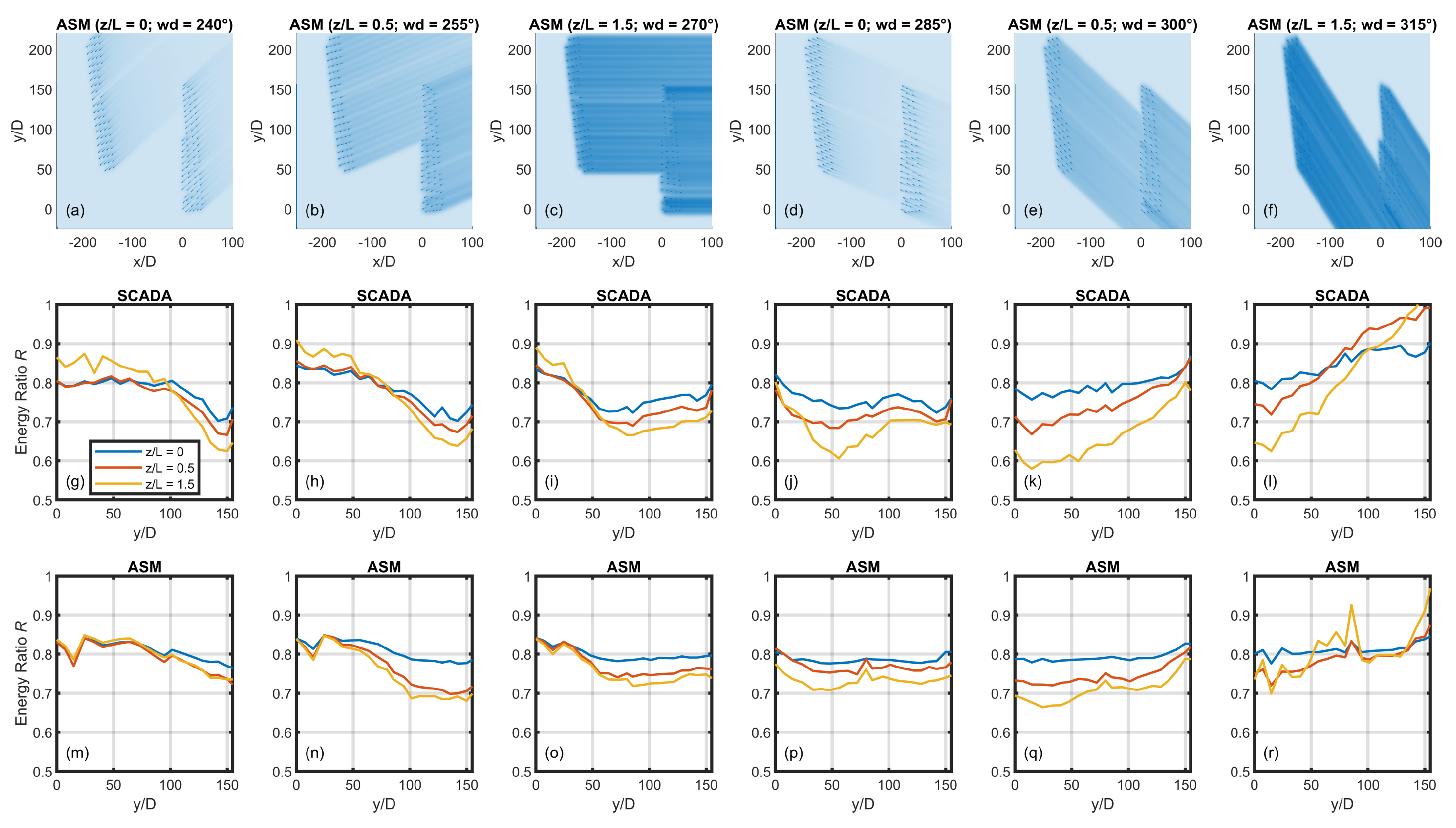
Figure 8a–f present ASM modelled two-dimensional wind speeds of the flow through the SAB wind farm whose wakes impact the DAT wind farm for a freestream wind speed of 8 m/s and Monin–Obukhov stability parameters of (a, d), (b, e), and (c, f). Figure 8a (f) illustrates that the far wake of Sandbank for a wind direction of 240 (315) impacts the northern (southern) part of DanTysk, with the southern (northern) part in theoretically freestream conditions (assuming a homogeneous flow field). The wind direction wake of 285 in Figure 8d in neutral conditions illustrates practically no effect on the downstream DAT wind farm consistent with our understanding that wind-farm far-wake lengths in neutral conditions amount to 15 km [35]. If correct, energy capture models can neglect wind farms further than 15 km away if only neutral conditions are to be considered. We discuss the panels g–f once more further below after presenting Figure 9 and Figure 10.
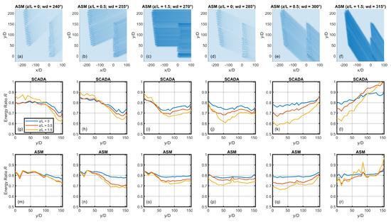
Figure 8.
The western north–south row of DanTysk for wind directions of 15 in increments from 240 to 315 from left to right, showing (a–f) two-dimensional ASM wind speeds for a freestream wind speed of 8 m/s, (g–l) the SCADA data, and (m–r) the ASM results. The lines show different Monin–Obukov stability parameters (blue), (red), and = 1.5 (yellow).
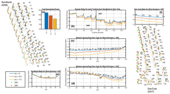
Figure 9.
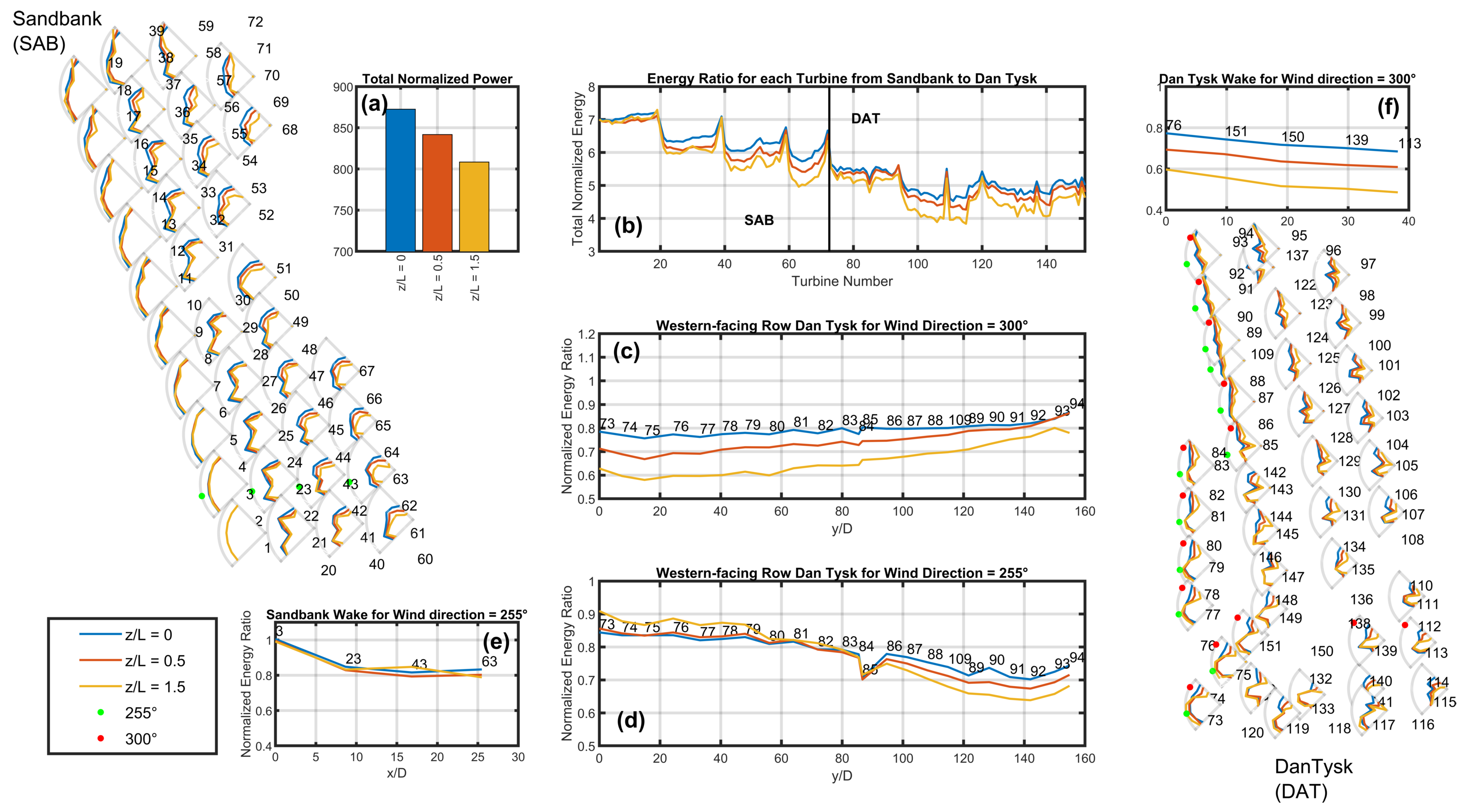
Partial polar plots (225–315) of normalized SCADA energy ratio (with respect to turbine 1 located at the south-west of Sandbank) for wind turbines of the SAB and DAT wind farms for Monin–Obukhov stability parameters of 0 (blue), 0.5 (red), and 1.5 (yellow). The polar plots are positioned at the relative positions of the wind turbines (numbers indicated) within the SAB and DAT wind farms. Note that only polar plots are shown for every second wind turbine due to space considerations. A bar chart of the summed energy ratios (a) is shown for all turbines of the SAB and DAT wind farms for each wind direction for a variation in stability. Presented in (b) are the summed energy ratios for each wind turbine (horizontal axis) of Sandbank (turbines 1 to 72) and DanTysk (turbines 73 to 152). The reference wind turbine number 1 gives a value of seven (it is the sum of an arc of a unit circle consisting of seven directions). The panels (c) and (d) show the energy ratio of the western row of DanTysk for wind directions of 300 and 255, respectively. Panels (e) and (f) are selected wake rows for those wind directions in the SAB and DAT wind farms, respectively. Green and red points on the polar plots highlight wind directions of 255 and 300 as plotted in panels (e,d) and (c,d), respectively.
Figure 10.
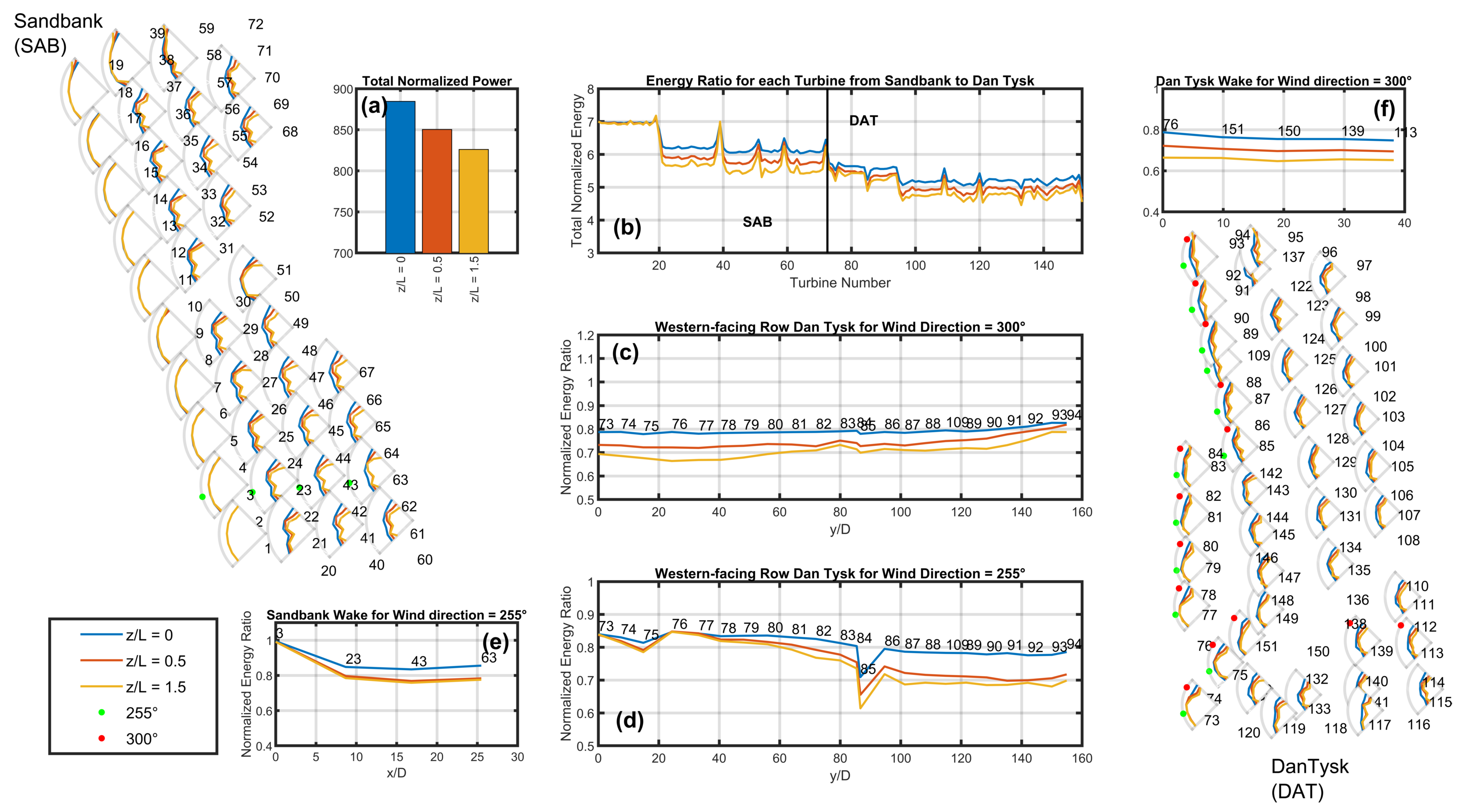
As Figure 9 but for the ASM results.
Figure 9 presents a similar representation of cluster N-5 to that presented in Figure 6 for cluster N-4 where partial polar plots of the energy ratio are placed in the layout of the farms. The energy ratios R in all polar plots are normalized by the energy ratio of turbine number 1 located to the south-west of Sandbank, with this plot giving the arc of a unit circle for seven wind directions in 15 increments from 225 to 315. Deviations from a unit arc are indicative of flow modifications due to wakes, upstream induction, or flow inhomogeneities. For example, the western row of Sandbank (turbines 1 to 19) are approximations to unit arcs assuming they see the freestream conditions in this wind direction sector equivalent to the flow seen by turbine number 1. In all plots, three curves are plotted to correspond to neutral (blue; = 0), stable (red; = 0.5), and strongly stable (yellow; = 1.5) conditions. From the polar plots in both wind farms, the effect of waking with increasing stability is seen as one progresses deeper west–east into the wind farm with energy ratio deficits favouring particular wind directions aligned with the positions of the upstream wind turbines. One of those directions is the wind direction 255 (marked by the green circles on the corresponding polar plots) for Sandbank for which the energy ratios of a selected row are presented in Figure 9e showing a reduction in power by 20% () after the front row for all stability classes. The ASM energy ratio in Figure 10e is a similar value ().
The partially waked western “front row” of DanTysk for this wind direction is presented in Figure 9d for neutral (blue), stable (red), and strongly stable (yellow) conditions with the turbine numbers of the row indicated at the positions of the turbines near the neutral blue curve. The spatial coordinates are normalized with respect to the southernmost turbine 73 in this row (see the polar plots). For this wind direction a wake represented by an energy deficit should be evident if one progresses from south () to north beginning at about turbine 84 () according to the modelled wind speeds shown previously (Figure 8b). Note that the value of the freestream energy ratio for the southern turbines is not unity because the DanTysk energy ratios are normalized with respect to turbine 1 located at Sandbank, which contains more powerful rated turbines (4 MW versus 3.6 MW; see Table 1). Therefore, we seek energy deficits as increases below an energy ratio of about 0.8–0.9, which is approximately DanTysk’s normalized freestream energy ratio with respect to Sandbank. Figure 9d shows a stability dependence, with the neutral case remaining at roughly the expected freestream value along the entire row, while the energy ratio of the strongly stable case reduces to about 0.6 for . The SCADA suggest a speed-up for the strongly stable case (yellow in panel d). Note that for this wind direction, turbine 85 is slightly waked by 84, which is responsible for the sharp dip in the curve seen at ( (for more northerly wind directions, turbine 85 is unwaked).
The second wind direction considered in more detail is 300 which should give the northern part of DanTysk in freestream conditions. Figure 9c shows that the northernmost turbines in the front row of DanTysk for 300 are approximately of the magnitude of the freestream energy ratios of 0.8. Further to the south (), the curves are quite ordered in a way suggestive of an increased effect of the Sandbank wake on DanTysk for increasing stability. The energy ratio for tends to be about 0.7 at and about 0.6 at for . Consequently, as parts of DanTysk’s front row suffer from an energy deficit due to the wake of Sandbank, and that deficit seems to propagate through the wind farm. For example, Figure 9f shows a selected row through the Dan Tysk wind farm beginning at turbine 76. Here, the strengths of the internal wakes appear independent of stability because the curves have similar slopes, but the initial energy in the front row results in an overall energy deficit that increases with stability within the DanTysk wind farm. This may also be evident from the front-row energy deficits for north-westerly wind directions in stable conditions seen in the DanTysk polar plots.
The summed energy for each wind turbine is presented in Figure 9b beginning at turbine 1 in Sandbank to the left of that panel with a value of seven (the number of wind directions considered) and continuing to turbine 151 within DanTysk. Figure 9b shows a consistent ordering with stability throughout the farms with more energy in neutral conditions, and energy decreasing for increasing stability. The total normalized energy shown in Figure 9a representing all turbine energy ratios summed for all wind directions and both farms shown here, gives a reduction in overall power by about 5% and 10% for stable and strongly stable conditions, respectively, compared with the neutral case.
Figure 10 presents the ASM results as polar plots in the same form as the SCADA results in Figure 9. Figure 10a reveals a similar reduction in power along the aligned Sandbank wake row at the wind direction of 255. Here, energy is reduced by about 20% of the freestream value for each stability, with the model giving a slight stability dependence. Figure 10b presents the summed energy ratio for each turbine in the cluster. The apparent north-west–south-east energy bias evident in the SCADA data is absent in the ASM results as expected for a homogenous inflow (see the constant power along the western rows of Sandbank (e.g., turbines 1 to 19). As the domain area of any model increases, we expect non-homogeneity of the freestream conditions to introduce a more significant error than far wakes in energy assessments. The peaks seen in Figure 10b (left of the vertical black line) are the turbines of Sandbank’s northern row (turbines 19, 39, 59, 72) and are less waked than the turbines further south and into the wind farm. Figure 10c presents the energy ratio of the western Sandbank row for a 300 flow, where there is a weaker negative south–north gradient evident in the modelling results compared with the energy ratios calculated from the SCADA data in Figure 9c. For a westerly flow, the SAB–DAT wind farm separation is about 20 km, whereas the north-west–south-east separation (between turbines 72 (SAB) and 73 (DAT) for example) extends to 30 km. The underestimated wake strength for the longer wake suggests the model could be improved. For and a wind direction of 300, the SCADA data tell us that the wake strength 30 km downstream from Sandbank is roughly 0.5/0.8 ≈ 63% (Figure 9c) of the expected freestream wake strength, with 63% being conveniently the e-folding distance assuming an exponential downstream wind speed recovery: the wake will recover to 95% of the freestream value at a factor of three times the e-folding distance, giving a wake length of roughly 90 km, which is possibly longer than anything measured to date.
On the other hand, for the westerly flow (255) in Figure 10d, the ASM approach gives a stability dependence broadly consistent with the SCADA data. For example, the SCADA data for in Figure 9d give energy ratios approaching 0.65 for but the ASM results proved energy ratios of about 0.7. Assuming freestream values are about 0.8, then we are detecting wake lengths in this direction in strongly stable conditions of about a length of 40 km assuming a full wind speed recovery to 95% of the freestream value. The weaker stability dependence is also evident in the modelled DAT wake results of Figure 10f, showing a weaker separation of the stability lines compared with the SCADA data shown in Figure 9f.
Returning to Figure 8, western-row DAT energy ratios are presented in panels g–l (SCADA) and panels m–r (ASM) corresponding to the wind directions shown in panels a–f. Here the progression of the far-wake effect at the DAT front row from north at 240 to south at 315 is evident: first the northern part of DanTysk is waked for south-westerlies and then the southern part for north-westerlies. In all wind directions, the ASM tends to capture the qualitative shape of the energy ratio in the waked region, but the dependence on stability is quantitatively weaker than suggested by the SCADA data. For example, for the wind direction of 270, there is a clear energy ratio deficit for about as we see from the wind speeds in (c), although the ASM energy ratios have a weaker stability dependence than that of the SCADA data. Speed-up is once more possibly evident in strongly stable conditions for (yellow curve). This is the consistent result of Figure 8 which shows a qualitatively similar wake effect between the SCADA and ASM, corresponding to the wind speeds in panels a–f, but the stability effect has been underestimated, particularly for the wind direction of 315.
5. Discussion
The presentation of SCADA data from four North Sea wind farms for different flow orientations has introduced the detection of, first, stability-dependent internal wakes and then stability-dependent wind-farm wakes in a sequential manner. Within the wind farm, wind turbine wakes produce a clear energy ratio deficit that increases with stability in the downstream-affected turbines. The NSO waked row in Figure 6a and Figure 7a gives a classical waked-row signature of maximum energy at the unwaked, upstream turbine and then a slightly reduced power with increasing distance downstream. In contrast, the ABW waked row in the denser wind farm (Figure 6c) gives a continually decreasing energy with increasing downstream distance from a maximum energy at the first unwaked wind turbine. The SCADA data supported by modelling results suggest an increasing energy deficit for increasing stability throughout the wind farm. Expectantly, the wind farm wakes propagate downstream as evident in the corresponding SCADA data of the neighboring wind farm: the NSO wind farm in the case of a north-westerly flow, and the ABW wind farm in the case of a south-westerly flow. That the wind-farm wake strength directly behind the farm increases with increasing stability from the SCADA results is expected from theoretical investigations of hypothetical large wind farms [26,27], and thus it follows that a clear wake signal for such a short (<5 km) distance would be evident, even for neutral conditions.
Application of the methodology used for analysis of the N-4 cluster to the N-5 cluster consisting of two wind farms separated by 20 km reveals wind farm wakes persisting for more than 20 km, and this is particularly evident in stable conditions. The length of such wakes in stable conditions is consistent with the stable wake lengths detected in flight measurements shown in Cañadillas et al. [35], even out to roughly 60 km, but here demonstrated directly from the wind turbine power measurements. The qualitative shape of the wakes is supported by the ASM described in Cañadillas et al. [37], but our initial prescription of that model based on slightly stable () LES results is likely underestimating the strength of such wakes when comparing the model with the SCADA power.
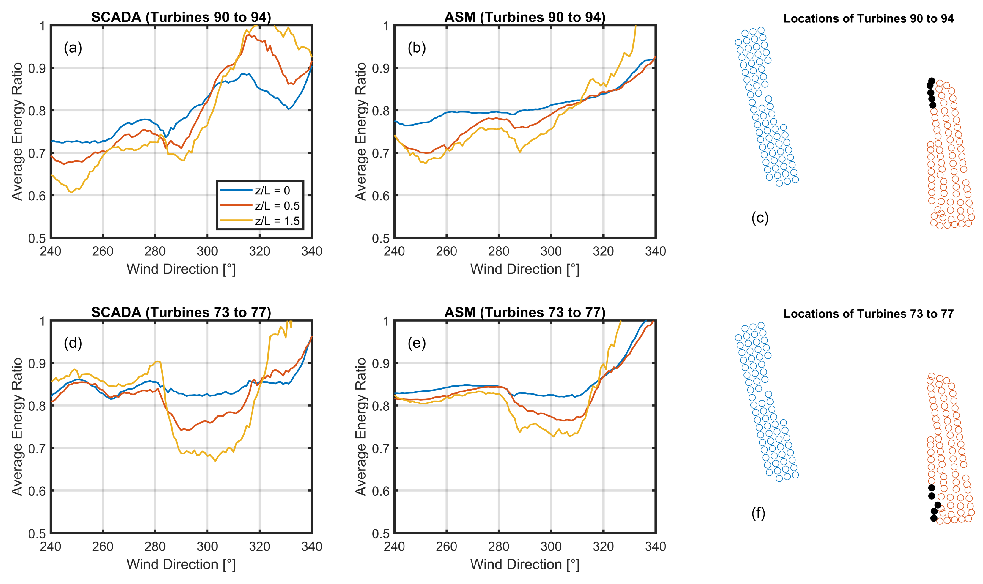
The stability-dependent far-wake effects can be viewed in the way shown in Figure 11, which presents the average energy ratio from five northern (top row) and southern (bottom row) turbines from the western row of DanTysk for freestream wind directions ranging from 240 to 340. Figure 11a,d and Figure 11b,e show the SCADA and ASM derived energy ratios, respectively, which have both been normalized with respect to turbine 1 at Sandbank as above (see Figure 9). For south-westerly winds (240–300), there is an increasing energy deficit seen in both SCADA and ASM results with stability in the northern wind turbines, which we interpret as wake effects as discussed above. A similar phenomenon is seen in the southern turbines for more northerly wind directions but for a narrower range (280–310) due to the upstream Sandbank layout. With the help of a simple engineering model, we are able to separate wake model effects from mere flow inhomogeneity which we see, for example, in Figure 11a beginning for wind directions of 300. The ASM results suggest a slowly increasing energy ratio with increasingly northern flow, whereas the SCADA results are suggestive of some type of flow speed-up just outside the wake region for a wind direction of approximately 310.
Figure 11.
Average energy ratios according to the SCADA (a,d) and ASM (b,e) results for five northern (c) and southern (f) turbines from DanTysk’s western row (black points) for wind directions 240–340. The energy ratios are normalized with respect to turbine 1 (SAB, see also Figure 6). Sandbank (blue) and DanTysk (red) are shown in (c,f).
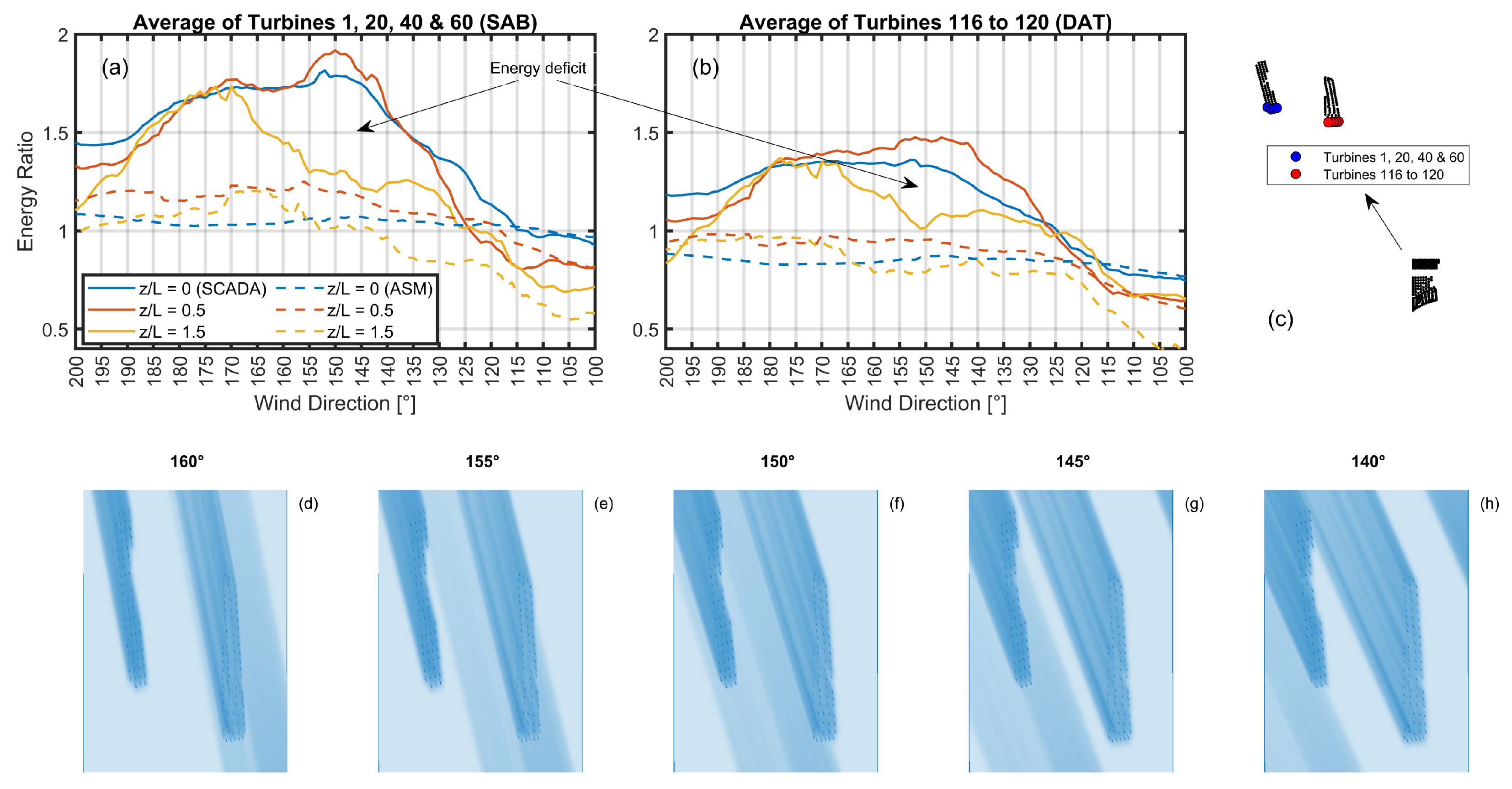
Extending this analysis even further for very long wakes between the N-4 and N-5 clusters as illustrated in the layouts of Figure 1 to detect any evidence of long wakes in the SCADA data there, we arrive at Figure 12. Figure 12a,b show the average turbine power for the southern rows of turbines in cluster N-5 as depicted in Figure 12c for flow from the south. The solid lines are SCADA results and the dashed the ASM results for neutral, stable and strongly stable conditions for wind directions between 100 and 200. Figure 12d to h show wind speeds at the N-5 cluster for a freestream wind speed of 8 m/s for the wind directions 160, 155, 150, 145, and 140 where we would expect any wake effects to be evident in the data if we neglect the Coriolis force. Here the reference wind direction is at the N-4 cluster, so the Coriolis force (flow turning to the right) would make it seem the wake effects are evident for wind directions more to the east. Figure 12a,b tentatively suggest a deficit in the SCADA results for at about the wind direction range expected. The ASM results (dashed lines) seem to have very tentatively captured the wake effect as evident from the line (yellow) but this is quite speculative at this stage. The ASM energy ratios are lower than the SCADA energy ratios because we know there is wind speed from the coast of up to 35% as documented previously [36,48]. Hence, when modelling such large-scale coastal areas, long-range wakes are probably of lesser significance with accounting for the correct flow inhomogeneity [31], which is why these speculative results are included here in the discussion. Further data analysis combined with more sophisticated modelling efforts (e.g., with LES or the mesoscale WRF model) may help to elucidate the combined far-wake and non-homogeneous aspects more clearly in SCADA results in the future.
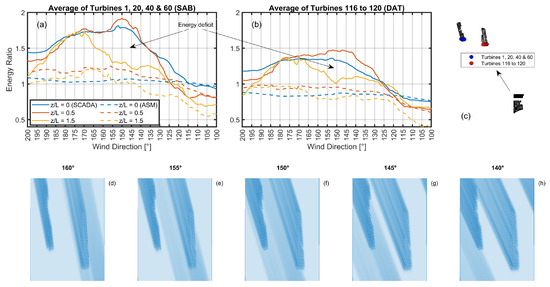
Figure 12.
Average energy ratios of the southern row turbines (a) 1, 20, 40, and 60 (SAB) and (b) 116 to 120 (DAT) for the SCADA data (solid lines) and ASM results (dashed lines) for flow from the N-4 cluster as indicated in panel (c), which shows the relative positions of the turbines with respect to N-4. The ASM wind speeds for from the N-4 cluster to N-5 according to the ASM approach is shown in panels (d–h) for the wind directions where wakes from N-4 are expected to affect N-5.
Since the ASM results produce quantitatively weaker wake effects compared with the SCADA results, we suppose this is because the model was inspired by LES results in only weakly stable conditions [37]. Hence, for practical applications, the ASM approach could (and probably should) be optimized to reproduce the stability-dependent internal and far wakes demonstrated here and other places for the purposes of accounting for stability in the energy yield forecasting of large wind farms. The specific application for such a model would be in future scenarios in which a prospective wind farm becomes increasingly affected by yet-to-built neighbouring wind farms, such as that which will occur in the crowded North Sea area.
6. Conclusions
Wind power measurements according to real SCADA data from a number of wind farms in the North Sea were cleaned, processed and analysed in order to detect the presence and atmospheric stability dependence of near (<5 km), far (≈20 km), and very far (∼60 km) wakes in downstream, neighboring offshore wind farms. Whereas similar atmospheric stability analyses have focused principally on the wind speed itself, here we are privileged to have had access to raw SCADA wind power data that reveal a consistent far-wake stability-dependent phenomena previously suggested by measurements of the wind speed via flight, satellite, or lidar measurement techniques or even modelling studies. Near wakes analysed at the offshore N-4 cluster in the North Sea containing an approximately 5 km-wide gap between the Amrumbank West and Nordsee Ost wind farms reveal a clear stability-dependent wake in the front-row downstream turbines. More interestingly, for far wakes we detect a reduction in power in the waked front-row part of the downstream wind farm by up to 25% in strongly stable () conditions, where the downstream wind farm in this case (DanTysk) is 20 km from the upstream wind farm (Sandbank) in the North Sea. In neutral conditions, the energy reduction is limited to at most 10% at the front row. With the use of Openwind, the recently developed ASM approach, which is far-wake engineering model for taking stability in the sense of Monin–Obukhov theory into account, is able to largely capture the qualitative aspects of far wakes but probably underestimates their stability dependence. Underestimated very far wakes by the ASM approach are possibly also found, since we detect a wake signal in the wind power data of the N-5 cluster (Sandbank and DanTysk) for flow from the more southern N-4 cluster (Amrumbank, Nordsee Ost, and Meerwind Sued|Ost). However, it appears that at this scale, nonhomogeneity of both speed and direction, including speed-up with increasing distance from the coast, is probably a more pressing issue for long-range engineering-based wake modelling. Our purposes here were to use the model for wake-recognition purposes in order to gauge the significance of stability-dependent wakes in operational conditions. We suggest the model is a useful first estimate for assessment of stability-dependent far-wake effects up to 30 km in length in crowded offshore wind farm areas but further optimization of the ASM approach could be conducted for real energy capture investigations.
Author Contributions
Both R.J.F. and B.C. and wrote the manuscript and evaluated and prepared the figures. N.R. performed the simulations in Openwind. All authors contributed intensively to an internal review. All authors have read and agreed to the published version of the manuscript.
Funding
This research has been supported by the X-Wakes project, funded by the Federal Ministry for Economic Affairs and Climate Action (BMWK) (grant no. FKZ 03EE3008 (A-G)).
Data Availability Statement
The data are not publicly available due to non-disclosure agreements.
Acknowledgments
The contribution of RWE and Vattenfall in providing the SCADA measurement data for the purposes of this research project is also gratefully acknowledged. At RWE’s and Vattenfall’s request, all power measurement data presented in this study have been normalised. The WRF results were made available by IWES as project partners in the X-Wakes project.
Conflicts of Interest
Authors Richard J. Foreman and Nick Robinson were employed by UL International. The remaining author declares that the research was conducted in the absence of any commercial or financial relationships that could be construed as a potential conflict of interest.
References
- Westerhellweg, A.; Cañadillas, B.; Kinder, F.; Neumann, T. Wake measurements at alpha ventus–dependency on stability and turbulence intensity. J. Phys. Conf. Ser. 2014, 555, 12106. [Google Scholar] [CrossRef]
- van der Laan, M.P.; García-Santiago, O.; Kelly, M.; Meyer Forsting, A.; Dubreuil-Boisclair, C.; Seim, K.S.; Imberger, M.; Peña, A.; Sørensen, N.N.; Réthoré, P.E. A new RANS-based wind farm parametrization and inflow model for wind farm cluster modeling. Wind Energy Sci. Discuss. 2022, 2022, 1–38. [Google Scholar]
- Porté-Agel, F.; Bastankhah, M.; Shamsoddin, S. Wind-Turbine and Wind-Farm Flows: A Review. Bound.-Layer Meteorol. 2020, 174, 1–59. [Google Scholar] [CrossRef] [PubMed]
- Lundquist, J.K.; DuVivier, K.K.; Kaffine, D.; Tomaszewski, J.M. Costs and consequences of wind turbine wake effects arising from uncoordinated wind energy development. Nat. Energy 2019, 4, 26–34. [Google Scholar] [CrossRef]
- Wu, Y.T.; Porté-Agel, F. Atmospheric turbulence effects on wind-turbine wakes: An LES study. Energies 2012, 5, 5340–5362. [Google Scholar] [CrossRef]
- Medici, D.; Ivanell, S.; Dahlberg, J.; Alfredsson, P.H. The upstream flow of a wind turbine: Blockage effect. Wind Energy 2011, 14, 691–697. [Google Scholar] [CrossRef]
- Vermeer, L.; Sørensen, J.; Crespo, A. Wind turbine wake aerodynamics. Prog. Aerosp. Sci. 2003, 39, 467–510. [Google Scholar] [CrossRef]
- Wu, K.L.; Porté-Agel, F. Flow adjustment inside and around large finite-size wind farms. Energies 2017, 10, 2164. [Google Scholar] [CrossRef]
- Christiansen, M.B.; Hasager, C.B. Wake effects of large offshore wind farms identified from satellite SAR. Remote Sens. Environ. 2005, 98, 251–268. [Google Scholar] [CrossRef]
- Cañadillas, B.; Beckenbauer, M.; Trujillo, J.J.; Dörenkämper, M.; Foreman, R.; Neumann, T.; Lampert, A. Offshore wind farm cluster wakes as observed by long-range-scanning wind lidar measurements and mesoscale modeling. Wind Energy Sci. 2022, 7, 1241–1262. [Google Scholar] [CrossRef]
- Fischereit, J.; Brown, R.; Larsén, X.G.; Badger, J.; Hawkes, G. Review of mesoscale wind-farm parametrizations and their applications. Bound.-Layer Meteorol. 2022, 182, 175–224. [Google Scholar] [CrossRef]
- Openwind|Wind Farm Modeling and Layout Design Software. Available online: https://www.ul.com/software/openwind-wind-farm-modeling-and-layout-design-software (accessed on 15 November 2023).
- Wind Farm Design and Analysis Software, Windfarmer. Available online: https://www.dnv.com/software/services/windfarmer/index.html (accessed on 15 November 2023).
- The World of WAsP by DTU Wind and Energy Systems. Available online: https://www.wasp.dk/ (accessed on 16 November 2023).
- AWS Truepower. Openwind Theoretical Basis and Validation; Technical Report; AWS Truepower: Albany, NY, USA, 2010. [Google Scholar]
- Jensen, N. A Note on Wind Generator Interaction; Risø National Laboratory: Roskilde, Denmark, 1983. [Google Scholar]
- Ainslie, J. Calculating the flowfield in the wake of wind turbines. J. Wind. Eng. Ind. Aerodyn. 1988, 27, 213–224. [Google Scholar] [CrossRef]
- Bastankhah, M.; Porté-Agel, F. A new analytical model for wind-turbine wakes. Renew. Energy 2014, 70, 116–123. [Google Scholar] [CrossRef]
- Pedersen, J.; Svensson, E.; Poulsen, L.; Nygaard, N. Turbulence Optimized Park model with Gaussian wake profile. J. Phys. Conf. Ser. 2022, 2265, 22063. [Google Scholar] [CrossRef]
- Frandsen, S. On the wind speed reduction in the center of large clusters of wind turbines. J. Wind. Eng. Ind. Aerodyn. 1992, 39, 251–265. [Google Scholar] [CrossRef]
- Emeis, S.; Frandsen, S. Reduction of horizontal wind speed in a boundary layer with obstacles. Bound.-Layer Meteorol. 1993, 64, 297–305. [Google Scholar] [CrossRef]
- Frandsen, S.; Barthelmie, R.; Pryor, S.; Rathmann, O.; Larsen, S.; Højstrup, J.; Thøgersen, M. Analytical modelling of wind speed deficit in large offshore wind farms. Wind Energy 2006, 9, 39–53. [Google Scholar] [CrossRef]
- Frandsen, S.T.; Jørgensen, H.E.; Barthelmie, R.; Rathmann, O.; Badger, J.; Hansen, K.; Ott, S.; Rethore, P.E.; Larsen, S.E.; Jensen, L.E. The making of a second-generation wind farm efficiency model complex. Wind Energy 2009, 12, 445–458. [Google Scholar] [CrossRef]
- Brower, M.; Robinson, N. The OpenWind Deep-Array Wake Model: Development and Validation; Technical Report; AWS Truepower: Albany, NY, USA, 2012. [Google Scholar]
- Gunn, K. Improvements to the Eddy Viscosity Wind Turbine Wake Model. J. Phys. Conf. Ser. 2019, 1222, 12003. [Google Scholar] [CrossRef]
- Emeis, S. A simple analytical wind park model considering atmospheric stability. Wind Energy 2010, 13, 459–469. [Google Scholar] [CrossRef]
- Peña, A.; Rathmann, O. Atmospheric stability-dependent infinite wind-farm models and the wake-decay coefficient. Wind Energy 2014, 17, 1269–1285. [Google Scholar] [CrossRef]
- Emeis, S. Current issues in wind energy meteorology. Meteorol. Appl. 2014, 21, 803–819. [Google Scholar] [CrossRef]
- Foreman, R.J.; Emeis, S.; Canadillas, B. Half-order stable boundary-layer parametrization without the eddy viscosity approach for use in numerical weather prediction. Bound.-Layer Meteorol. 2015, 154, 207–228. [Google Scholar] [CrossRef]
- Emeis, S.; Siedersleben, S.; Lampert, A.; Platis, A.; Bange, J.; Djath, B.; Schulz-Stellenfleth, J.; Neumann, T. Exploring the wakes of large offshore wind farms. J. Phys. Conf. Ser. 2016, 753, 092014. [Google Scholar] [CrossRef]
- Emeis, S. Analysis of Some Major Limitations of Analytical Top-Down Wind-Farm Models. Bound.-Layer Meteorol. 2023, 187, 423–435. [Google Scholar] [CrossRef]
- Fitch, A.C.; Olson, J.B.; Lundquist, J.K.; Dudhia, J.; Gupta, A.K.; Michalakes, J.; Barstad, I. Local and mesoscale impacts of wind farms as parameterized in a mesoscale NWP model. Mon. Weather. Rev. 2012, 140, 3017–3038. [Google Scholar] [CrossRef]
- Nygaard, N.G.; Steen, S.T.; Poulsen, L.; Pedersen, J.G. Modelling cluster wakes and wind farm blockage. J. Phys. Conf. Ser. 2020, 1618, 62072. [Google Scholar] [CrossRef]
- Siedersleben, S.K.; Platis, A.; Lundquist, J.K.; Lampert, A.; Bärfuss, K.; Cañadillas, B.; Djath, B.; Schulz-Stellenfleth, J.; Bange, J.; Neumann, T.; et al. Evaluation of a Wind Farm Parametrization for Mesoscale Atmospheric Flow Models with Aircraft Measurements. Meteorol. Z. 2018, 27, 401–415. [Google Scholar] [CrossRef]
- Cañadillas, B.; Foreman, R.; Barth, V.; Siedersleben, S.; Lampert, A.; Platis, A.; Djath, B.; Schulz-Stellenfleth, J.; Bange, J.; Emeis, S.; et al. Offshore wind farm wake recovery: Airborne measurements and its representation in engineering models. Wind Energy 2020, 23, 1249–1265. [Google Scholar] [CrossRef]
- Djath, B.; Schulz-Stellenfleth, J.; Cañadillas, B. Study of Coastal Effects Relevant for Offshore Wind Energy Using Spaceborne Synthetic Aperture Radar (SAR). Remote Sens. 2022, 14, 1688. [Google Scholar] [CrossRef]
- Cañadillas, B.; Foreman, R.; Steinfeld, G.; Robinson, N. Cumulative interactions between the global blockage and wake effects as observed by an engineering model and large-eddy simulations. Energies 2023, 16, 2949. [Google Scholar] [CrossRef]
- Forschungsplattformen in Nord- und Ostsee Nr. 1,2,3. Available online: https://www.fino-offshore.de/de/index.html (accessed on 21 November 2023).
- Doekemeijer, B.M.; Simley, E.; Fleming, P. Comparison of the Gaussian wind farm model with historical data of three offshore wind farms. Energies 2022, 15, 1964. [Google Scholar] [CrossRef]
- Rodrigo, J.S.; Cantero, E.; García, B.; Borbón, F.; Irigoyen, U.; Lozano, S.; Fernande, P.; Chávez, R. Atmospheric stability assessment for the characterization of offshore wind conditions. J. Phys. Conf. Ser. 2015, 625, 12044. [Google Scholar] [CrossRef]
- von Brandis, A.; Centurelli, G.; Schmidt, J.; Vollmer, L.; Djath, B.; Dörenkämper, M. An investigation of spatial wind direction variability and its consideration in engineering models. Wind Energy Sci. 2023, 8, 589–606. [Google Scholar] [CrossRef]
- Branlard, E.; Gaunaa, M. Cylindrical vortex wake model: Right cylinder. Wind Energy 2015, 18, 1973–1987. [Google Scholar] [CrossRef]
- Troldborg, N.; Meyer Forsting, A. A simple model of the wind turbine induction zone derived from numerical simulations. Wind Energy 2017, 20, 2011–2020. [Google Scholar] [CrossRef]
- Gribben, B.J.; Hawkes, G.S. A Potential Flow Model for Wind Turbine Induction and Wind Farm Blockage; Technical Report; Frazer-Nash Consultancy: Leatherhead, UK, 2019. [Google Scholar]
- Stull, R.B. An Introduction to Boundary Layer Meteorology; Springer: Berlin/Heidelberg, Germany, 1988. [Google Scholar]
- Emeis, S. Wind Energy Meteorology: Atmospheric Physics for Wind Power Generation; Springer: Berlin/Heidelberg, Germany, 2018. [Google Scholar]
- Nygaard, N.G.; Hansen, S.D. Wake effects between two neighbouring wind farms. J. Phys. Conf. Ser. 2016, 753, 32020. [Google Scholar] [CrossRef]
- Cañadillas, B.; Wang, S.; Ahlert, Y.; Djath, B.; Barekzai, M.; Foreman, R.; Lampert, A. Coastal horizontal wind speed gradients in the North Sea based on observations and ERA5 reanalysis data. Meteorol. Z. 2023, 32, 207–228. [Google Scholar] [CrossRef]

Disclaimer/Publisher’s Note: The statements, opinions and data contained in all publications are solely those of the individual author(s) and contributor(s) and not of MDPI and/or the editor(s). MDPI and/or the editor(s) disclaim responsibility for any injury to people or property resulting from any ideas, methods, instructions or products referred to in the content. |
© 2024 by the authors. Licensee MDPI, Basel, Switzerland. This article is an open access article distributed under the terms and conditions of the Creative Commons Attribution (CC BY) license (https://creativecommons.org/licenses/by/4.0/).