Low-Carbon Optimization Scheduling of Integrated Energy Systems Based on Bilateral Demand Response and Two-Level Stackelberg Game

Abstract

In the context of low-carbon energy transformation, fully utilizing the integrated demand response (IDR) resources on the load side can improve the operational flexibility and economy of the integrated energy system (IES). However, establishing a reasonable trading mechanism to enhance users’ participation in IDR has become a key issue that IES urgently needs to solve. To this end, this paper first establishes an IES model that includes electricity, heat, and gas. To reduce carbon emissions, a ladder-type carbon trading mechanism is introduced while adding low-carbon technologies such as carbon capture devices and power-to-gas conversion. Secondly, a bilateral IDR mechanism centered on the load aggregator (LA) is proposed, and a multi-agent operation model including IES, LA, and users is established. The IDR subsidy price is dynamically determined through a two-level Stackelberg game model involving IES, LA, and users. Then, through KKT conditions and the Big M method, the two-level game model is turned into an IES-LA game model, which is solved using a combination of the White Shark Optimization method and the Gurobi solver. The final simulation results show that the scheduling model can fully reflect the time value of IDR resources, and the IES cost is decreased by USD 152.22, while LA and user benefits are increased by USD 54.61 and USD 31.85. Meanwhile, the ladder-type carbon trading mechanism and low-carbon technology have effectively achieved low-carbon operation of the system.

1. Introduction

Recently, the clean, efficient, and sustainable energy exploitation and utilization model has become an important development direction for the future energy field [1]. In terms of carbon peaking and carbon neutrality, integrated energy systems (IESs) can fully leverage the comprehensive advantages of various complementary energy sources, which is an effective way to achieve the transition from traditional power grids to smart grids. With the widespread integration of diverse loads, how to unleash the flexibility of demand-side resources and promote source-load friendly interaction is an important issue that IES needs to consider [2]. At present, integrated demand response (IDR) is one of the most effective methods [3], and the literature [4,5] shows that IDR guides users to use energy scientifically and reasonably through economic subsidies, playing an important role in balancing supply and demand. However, when users directly trade with IES, they will incur greater risks due to insufficient load balancing capacity, while IES needs to monitor a large number of users in real time, and the scheduling process is highly time-sensitive, which is difficult to solve by conventional techniques [6].

With the gradual maturity of the electricity market, most small- and medium-sized users trade IDR resources with IES through load aggregators (LA) [7]. As a bridge between users and IES, LA achieves cross-system scheduling of IDR resources through a bilateral IDR mechanism, which involves developing an IDR mechanism to aggregate users’ IDR resources and participating in IES’s IDR plan [8]. Literature [9] established a two-level optimization model between the distribution system operator (DSO) and LA, and the results showed that the two-level optimization scheduling model can fully exploit the regulation potential of LA and improve the revenue of both DSO and LA. Literature [10] proposed a hierarchical load scheduling framework that aggregates uninterrupted time shifting loads to optimize the operating costs of LA and DSO. Literature [11] considered community users as user aggregators (UAs) and investigated the energy interaction between community-integrated energy service providers and UA. Literature [12] proposed an optimization scheduling model for IES considering DR, with the objectives of maximizing the profits for both IES and LA. The above research achieved energy interaction between LA and IES but ignored the research of users’ interests. Literature [13] proposed an LA optimization model with the goal of maximizing users’ satisfaction and also established a pricing strategy model for IES with the goal of maximizing profits. Literature [14] developed an optimization scheduling model between the DSO, EV aggregator, and EV users and analyzed the impact of the EV aggregator’s operation mechanism on the interests of the three parties. The above research achieved the interaction of energy and benefits among energy suppliers, LA, and users through a bilateral IDR mechanism. However, the subsidy price of IDR is fixed, which cannot reflect the time value of IDR resources and cannot fully mobilize the enthusiasm of users.

In recent years, game theoretical methods have been more widely applied in IES energy price decision making and multi-subject interaction. Literature [15] established a trading strategy model between IES, LA, and users based on the master–slave game, which achieves the efficient use of DR resources by gaming the DR subsidy price. In order to achieve the balance of interests among IES operators, LA, and users, literature [16] established a hierarchical Stackelberg game model based on the consideration of users’ psychology. Reference [17] proposed a three-level framework for auxiliary service market operators, aggregators, and users and utilized the Stackelberg game model to achieve optimization scheduling of various auxiliary services, including demand response. The above studies have employed game theory methods to dynamically determine DR subsidy prices, reflecting the time value of DR resources. However, these studies only considered electricity DR resources and ignored the effective interaction between other DR resources such as heat and natural gas.

In addition, with the increasing severity of global warming, increasing the use of clean energy to reduce carbon emissions is a key issue for IES. The current research mainly focused on two aspects: innovative system architecture and the introduction of carbon trading mechanisms. In terms of IES system architecture, existing studies tend to introduce multiple low-carbon technologies to reduce system carbon emissions through multi-energy complementary and gradient utilization. Literature [18,19,20] showed that carbon capture systems (CCSs) and power to gas (P2G), as the most promising decarbonization technologies, can effectively reduce carbon emissions in the energy sector. Literature [21] added P2G and CCS to combined heat and power (CHP) and established an IES low-carbon optimization scheduling model. The simulation results showed that the carbon transaction cost of the system was reduced by 61.34%, the carbon emission was reduced by 3.94%, and the operating cost was reduced by 50.49%. In terms of the carbon trading mechanism, literature [22] developed an energy interaction and carbon trading mechanism between community IES, which reduced the overall operating costs and carbon emission costs. Literature [23] proposed a low-carbon economic operation strategy for IES based on a ladder-type carbon trading mechanism and carbon cycle, which realized the low-carbon use of energy. The above studies have effectively controlled the carbon emissions of IES in different ways, but there are fewer studies that combine multiple low-carbon technologies with carbon trading mechanisms in IES to achieve a reduction in systematic carbon emissions.

Additionally, there are many uncertainties in the operation of IES, such as the output of PV and WT. Existing research typically employs scenario analysis, stochastic programming, and robust optimization methods to simulate the effects of uncertain factors. Literature [24] used the Monte Carlo method to generate typical scenarios of PV in high-speed railway stations. Literature [25] considered the uncertainty of renewable energy output and used Latin hypercube sampling for simulation. However, the scheduling scheme obtained using the scenario analysis method cannot meet the optimal scheduling scheme for all scenarios. Literature [26] used a two-stage stochastic programming method to address the uncertainty of renewable energy output. However, both stochastic programming and scenario analysis methods require deterministic probability curves to generate scenarios, which may result in models that are not accurate enough to reflect actual situations. The robust optimization method replaces the exact probability distribution of random variables with uncertain sets and obtains the scheduling scheme of the system in the “worst-case” scenario through optimization methods, which is more in line with the needs of practical engineering. Literature [27] used robust optimization to describe the uncertainty of renewable energy output and promoted flexibility in the planning of the system. Literature [28] introduced robust optimization methods to handle electricity price uncertainty, which can maintain the conservatism of the optimization results at a relatively low level. It can be seen that robust optimization methods have broad application prospects in the scheduling decision-making problem of power systems because they do not require precise probability distribution information of uncertain parameters and can calculate quickly.

In summary, the existing research has the following shortcomings: (1) There is little study on the dynamic decision making of IDR subsidy prices in the multi-agent interaction model involving IES, LA, and users. (2) There is relatively little research on the integration of carbon trading mechanisms and various low-carbon technologies within IES to reduce system carbon emissions, and the carbon reduction capacity of IES needs further exploration. In response to the above issues, this paper proposes an integrated energy system low-carbon optimization scheduling model based on a bilateral demand response and two-level Stackelberg game. Therefore, the main contributions of this paper are as follows:

(1) By combining a ladder-type carbon trading mechanism with low-carbon technologies such as P2G and CCS, the low-carbon operation of IES can be promoted.

(2) A bilateral IDR incentive mechanism centered on LA is proposed, establishing a two-level Stackelberg game model that includes IES, LA, and users to dynamically determine IDR subsidy prices. Additionally, robust optimization method is utilized to address the uncertainty of wind turbine (WT) output within IES.

(3) By using the Karush–Kuhn–Tucke (KKT) condition and the Big M method, the two-level game model that includes IES, LA, and users is transformed into a game model between IES and LA. The White Shark Optimization (WSO) algorithm is combined with the Gurobi solver to solve the problem.

This paper consists of six parts. The energy flow structure and equipment model will be explained in Section 2. Section 3 introduces the bilateral IDR trading mechanism and establishes a multi-agent optimization model. Section 4 analyzes the two-level Stackelberg game formed between IES, LA, and users, Section 5 introduces the solution of the game model, and Section 6 conducts case analysis. Finally, the conclusion is drawn in Section 7.

2. Energy Flow and Device Model

2.1. IES Energy Flow

The energy flow inside IES is shown in Figure 1, and the main equipment includes renewable energy, CHP units for natural gas sources, gas boilers (GBs), a garbage incineration device, demand response, and energy storage systems (ESSs). Among them, CHP is composed of a gas turbine (GT) and a waste heat boiler (WHB) internally. To reduce carbon emissions, CCS and P2G devices have been added to the CHP unit. Specifically, the CCS unit captures the carbon dioxide generated during the combustion of the CHP unit and provides it to the P2G device to generate natural gas. The garbage incineration device is an ecologically beneficial controlled power generating unit that has the properties of reduction, harmless treatment, and resource utilization [22]. However, the large amount of harmful gas generated during the incineration process needs to be treated with flue gas before it can be discharged. This paper adds gas storage devices to achieve decoupling between the output of the garbage incineration device and flue gas treatment. At the same time, the distribution network and natural gas network provide electricity and natural gas to IES to ensure the normal operation of the system.

2.2. Device Model

2.2.1. CCS-P2G-CHP Model

(1) CHP model

In CHP units, GT burns natural gas to provide electricity and heat to various components of the system [29]. The relationship between its power generation and natural gas consumption is as follows:

$$P_{e,t}^{GT}=P_{g,t}^{GT}{\eta }_{GT}{Q}_{C{H}_4}$$

(1)

$$P_{\min }^{GT}\le P_{e,t}^{GT}\le P_{\max }^{GT}$$

(2)

where $P_{e,t}^{GT}$ is the electrical energy generated by the GT, $P_{g,t}^{GT}$ is the consumption of natural gas, ${\eta }_{CHP}$ is the power generation efficiency, and $Q_{C{H}_4}$ is the combustion heat value of natural gas. $P_{\max }^{GT}$ and $P_{\min }^{GT}$ are the upper and lower limits of GT power generation, respectively. Considering the cogeneration power of the CHP has the constraint of “determining electricity based on heat”, the heat power $P_{h,t}^{GT}$ of the GT can be expressed as follows:

$$\max \{P_{\min }-h_1{P}_{h,t}^{GT},h_m(P_{h,t}^{GT}-P_{h,o}^{GT})\}\le P_{e,t}^{GT}\le P_{\max }-h_2{P}_{h,t}^{GT}$$

(3)

where $P_{h,t}^{GT}$ is the heat generation power of the GT, $h_1$ and $h_2$ are the thermoelectric conversion coefficients corresponding to the minimum output power $P_{\min }$ and the maximum output power $P_{\max }$, and $h_m$ is the linear supply slope of the CHP thermoelectric power. $P_{h,o}^{GT}$ is the thermoelectric power corresponding to the lowest generation power of the GT.

The heat generation power of GB is the following:

$$P_{h,t}^{GB}=P_{g,t}^{GB}{\eta }_{GB}{Q}_{C{H}_4}$$

(4)

where $P_{g,t}^{GB}$ is the natural gas consumption, and ${\eta }_{GB}$ is the heat production efficiency.

(2) CCS-P2G model

This paper uses CCS to capture carbon dioxide generated during the production process of CHP units and transfers it to P2G devices. The electrical power $P_t^{CCS}$ consumed by CCS is directly proportional to the amount of carbon dioxide captured, and the expression is as follows:

$$P_t^{CCS}=\gamma W_t^{P2G}$$

(5)

$$W_t^{P2G}={\alpha }_{c{o}_2}{\eta }_{P2G}{P}_t^{P2G}$$

(6)

$$P_{\min }^{CCS}<P_t^{CCS}<P_{\max }^{CCS}$$

(7)

$$P_{\min }^{P2G}<P_t^{P2G}<P_{\max }^{P2G}$$

(8)

where $\gamma$ is the conversion coefficient of the electrical energy consumed to capture carbon dioxide, $W_{i,t}^{P2G}$ is the amount of carbon dioxide required for P2G, ${\alpha }_{c{o}_2}$ represents the amount of carbon dioxide required to generate unit power of natural gas, ${\eta }_{P2G}$ represents the conversion efficiency of P2G equipment, and $P_t^{P2G}$ represents the energy consumption of P2G equipment; $P_{\min }^{CCS}$ and $P_{\max }^{CCS}$ are the lower and upper limits of CCS power consumption, respectively. $P_{\min }^{P2G}$ and $P_{\max }^{P2G}$ are the lower and upper limits of the power consumption of P2G, respectively. $P_{g,t}^{P2G}$ is the amount of natural gas generated by the P2G device, expressed as follows:

$$P_{g,t}^{P2G}={\displaystyle \frac{3.6{\eta }^{P2G}{P}_t^{P2G}}{H^g}}$$

(9)

where $H^g$ is the calorific value of natural gas.

2.2.2. IDR Model

The multiple loads studied in this paper are electricity, heat, and gas. IDR resources include transferable loads and substitutable loads, and substitutable loads represent the ability of different types of energy to replace each other [30]. Any load within IES consists of three parts: fixed load, translatable load, and alternative load, which can be expressed as follows:

$$P_{j,t}^{load}=P_{j,t}^f+P_{j,t}^m+P_{j,t}^s$$

(10)

where $j$ represents the type of load, and $j\in \{e,h,g\}$, $e,h,g$ represent electricity, heat, and gas, respectively. $P_{j,t}^{load}$ represents the amount of class $j$ load. $P_{j,t}^f$ represents the fixed load, $P_{j,t}^m$ represents the translatable load, and $P_{j,t}^s$ represents the alternative load.

2.2.3. Garbage Incineration Device Model

In the flue gas treatment system of the garbage incineration device, the reaction tower processes the flue gas that enters through the smoke exhaust pipe and gas storage device, ensuring that pollutant gases in the flue gas are removed before emission. The ratio of the amount of flue gas entering the reaction tower to the amount of flue gas produced is the flue gas separation ratio ${\lambda }_t$ [31]. The amount of flue gas flowing into the gas storage tank can be adjusted by adjusting ${\lambda }_t$, as shown below:

$${\alpha }_t=P_t^{WI}{e}_{\alpha }={\alpha }_t^1+{\alpha }_t^2$$

(11)

$$P_t^{\alpha }=w^{\alpha }({\alpha }_t^1+{\alpha }_t^2)$$

(12)

$${\lambda }_t={\alpha }_t^1/{\alpha }_t$$

(13)

where ${\alpha }_t$ represents the amount of flue gas generated during incineration. ${\alpha }_t^1$ and ${\alpha }_t^2$ represent the amount of flue gas flowing into the reaction tower and storage tank, respectively. $P_t^{WI}$ is the output of the garbage incineration device, and $e_{\alpha }$ is the amount of flue gas generated per unit of electrical energy. $P_t^{\alpha }$ is the energy consumption of the flue gas treatment system, and $w^{\alpha }$ is the unit processing energy consumption coefficient of the flue gas treatment system.

2.2.4. ESS

The power expression for electric and heat energy storage is as follows:

$$E_{j,t}^{ES}=(1-{\eta }_{j,loss})E_{j,t-1}^{ES}+(\eta P_{j,t}^{cha}-{\displaystyle \frac{1}{\eta }}{P}_{j,t}^{dis})\Delta t$$

(14)

$$E_{j,\min }^e\le E_{j,t}^{ES}\le E_{j,\max }^e$$

(15)

$$0\le P_{j,t}^{cha}\le U_{j,t}^{es}{P}_{j,\max }^{cha}$$

(16)

$$0\le P_{j,t}^{dis}\le (1-U_{j,t}^{es})P_{j,\max }^{dis}$$

(17)

where $j$ represents the type of energy storage, and $j\in \{e,h\}$, $e,h$ represent electrical energy and heat energy, respectively. $E_{j,t}^e$ is the stored energy, ${\eta }_{j,loss}$ is the energy loss coefficient, and $\eta$ is the efficiency of charging and discharging energy. $P_{j,t}^{cha}$ and $P_{j,t}^{dis}$ are the power of charging and discharging energy, respectively. $E_{j,\min }^e$ and $E_{j,\max }^e$ are the minimum/maximum remaining capacity allowed during the scheduling process. $P_{j,\max }^{cha}$ and $P_{j,\max }^{dis}$ represent the upper limit of energy power for charging and discharging, and $U_{j,t}^{es}$ represents the state of charging and discharging, with a charging value of 1 and a discharging value of 0.

3. A Multi-Agent Optimization Model Considering Bilateral IDR Trading Mechanism

3.1. Bilateral IDR Trading Mechanism

This paper establishes a bilateral IDR trading mechanism, as shown in Figure 2, involving three types of stakeholders: IES, LA, and users. IES has established incentive mechanisms to provide LA with subsidy prices for IDR resources. As the integrator of load response resources, LA maximizes its own interests through a bilateral IDR mechanism. On the one hand, it signs contracts with IES to integrate IDR resources; on the other hand, it signs contracts with users to aggregate their load response by providing IDR subsidies. Users are the ultimate participants in IDR, and they gain economic benefits from the IDR platform provided by LA by adjusting the usage time of the load.

3.2. IES Model

3.2.1. IES Objective Function

$$\min C^{IES}={\displaystyle \sum _{t=1}^T{C}_t^{CHP}+}{C}_t^{utility}+C_t^{C{0}_2}+C_t^{IDR}$$

(18)

(1)

The operating cost of CCS-P2G-CHP unit $C_t^{CHP}$

$$C_t^{CHP}=a{P}_{e,t}^{GT}+b{(P_{e,t}^{GT})}^2+m_1{P}_t^{P2G}+m_2{P}_t^{CCS}+c$$

(19)

where $a,b,c$ are the operating cost coefficient of the CCS-P2G-CHP coupling system, and $m_1$ and $m_2$ are the operating and maintenance cost coefficients of P2G and CCS [32], respectively.

(2)

External interaction costs $C_i^{utility}$

External interaction cost includes natural gas purchase cost and electricity purchase cost:

$$C_i^{utility}={\displaystyle \sum _{t=1}^T{\lambda }_{g,t}^{buy}{P}_{g,t}^{buy}+{\lambda }_{e,t}^{buy}{P}_{e,t}^{buy}}$$

(20)

where ${\lambda }_{g,t}^{buy}$ and $P_{g,t}^{buy}$ are the purchase price and amount of natural gas; ${\lambda }_{e,t}^{buy}$ and $P_{e,t}^{buy}$ represent the purchase price and amount of electricity.

(3)

Ladder-type carbon trading cost $C_t^{C{O}_2}$

The carbon emission quota $W_t^0$ of IES is calculated by the following formula:

$$W_t^0=D(P_{e,t}^{GT}+P_{h,t}^{GT}+P_{h,t}^{GB}+P_t^{WI}+P_t^{WT})$$

(21)

where $D$ is the carbon emission quota for unit electricity and heat energy production; $P_t^{WT}$ is the power generated by WT.

IES carbon dioxide emissions $W_t^{c{o}_2,a}$ are modeled as follows:

$$W_t^{c{o}_2,a}=a_{c{o}_2}(P_{e,t}^{GT}+h_1{P}_{h,t}^{GT})+b_{c{o}_2}{P}_{h,t}^{GB}+c_{c{o}_2}{P}_t^{WI}-W_t^{P2G}$$

(22)

where $a_{c{o}_2}$, $b_{c{o}_2}$, and $c_{c{o}_2}$ are the carbon dioxide emission coefficients of CHP units, GB, and garbage incineration devices [33,34].

In summary, the carbon trading amount of IES is the following:

$$W_t^{c{o}_2}=W_t^{c{o}_2,a}-W_t^0$$

(23)

The ladder-type carbon trading mechanism divides multiple carbon emission right purchase intervals, and as IES needs to purchase more carbon emission right quotas, the purchase price of the corresponding interval will be higher. The ladder-type carbon trading model is the following:

$$C_t^{C{O}_2}=\left\{\begin{array}{l}\lambda W_t^{C{O}_2},W_t^{C{O}_2}\le l\\ \lambda (1+\alpha )(W_t^{C{O}_2}-l)+\lambda l,l<W_t^{C{O}_2}<2l\\ \lambda (1+2\alpha )(W_t^{C{O}_2}-2l)+(2+\alpha )\lambda l,2l<W_t^{C{O}_2}<3l\\ \lambda (1+3\alpha )(W_t^{C{O}_2}-3l)+(3+3\alpha )\lambda l,3l<W_t^{C{O}_2}<4l\\ \lambda (1+4\alpha )(W_t^{C{O}_2}-4l)+(4+6\alpha )\lambda l,4l<W_t^{C{O}_2}\end{array}\right.$$

(24)

where $\lambda$ is the carbon trading base price, $l$ is the interval length of carbon emissions, and $\alpha$ is the price increase rate.

(4)

IDR cost $C_t^{IDR}$

$$C_t^{IDR}=c_{e,t}^{IES}{P}_{e,t}^{LA}+c_{h,t}^{IES}{P}_{h,t}^{LA}+c_{g,t}^{IES}{P}_{g,t}^{LA}$$

(25)

Here, $c_{e,t}^{IES},c_{h,t}^{IES}$, and $c_{g,t}^{IES}$ are the unit electricity DR, heat energy DR, and natural gas DR subsidy price provided by IES to LA, while $P_{e,t}^{LA},P_{h,t}^{LA}$, and $P_{g,t}^{LA}$ are the electricity DR, heat DR, and natural gas DR aggregated by LA.

3.2.2. IES Constraint Condition

(1) IDR constraints

$$0\le P_{j,t}^{LA}\le P_{j,max}^{LA}$$

(26)

$$c_{j,\min }^{IES}\le c_{j,t}^{IES}\le c_{j,\max }^{IES}$$

(27)

Here, $j\in \{e,h,g\}$ represents the type of DR resources; $e,h$ and $g$ represent electricity, heat, and natural gas, respectively. $P_{j,max}^{LA}$ is the upper limits of the load response aggregated by LA, and $c_{j,\min }^{IES}$ and $c_{j,\max }^{IES}$ represent the minimum and maximum subsidy prices provided by IES.

(2) Electric power balance constraint

$$P_{e,t}^{load}=P_{e,t}^{buy}+P_{e,t}^{GT}+P_t^{WI}+P_t^{WT}+P_{e,t}^{LA}+P_{e,t}^{dis}-P_{e,t}^{cha}-P_t^{\alpha }-P_t^{P2G}-P_t^{CCS}$$

(28)

(3) Heat power balance constraint

$$P_{h,t}^{load}=P_{h,t}^{GT}+P_{h,t}^{GB}+P_{h,t}^{cha}+P_{h,t}^{LA}+P_{h,t}^{dis}$$

(29)

(4) Natural gas balance constraint

$$P_{g,t}^{load}=P_{g,t}^{buy}+P_{g,t}^{P2G}+P_{g,t}^{LA}-P_{g,t}^{GT}-P_{g,t}^{GB}$$

(30)

3.2.3. Uncertainty Model of WT Output

In practical operation, renewable energy connected to IES has uncertainty. Due to the many factors that affect uncertainty, it is easier to obtain uncertainty intervals in practical engineering. Therefore, this paper uses robust intervals to describe the uncertainty range of renewable energy output, as follows:

$$P_{WT}(t)=[{\overline{P}}_{WT}(t)-P_{WT}^{ld},{\overline{P}}_{WT}(t)+P_{WT}^{ud}]$$

(31)

where $P_{WT}(t)$ is the actual output of WT, ${\overline{P}}_{WT}(t)$ is the predicted value of WT, and $P_{WT}^{ld}$ and $P_{WT}^{ud}$, respectively, represent the maximum allowable deviation of WT. Due to the inability to directly find the expression of the worst case corresponding to the power balance constraint (28), an analytical expression for the worst-case power balance constraint is constructed based on the robust optimization method proposed in reference [35], as follows:

$$\begin{array}{cc}{P}_{e,t}^{load}\hfill & =P_{e,t}^{buy}+P_{e,t}^{GT}+P_t^{WI}+\max P_t^{WT}+P_{e,t}^{LA}+P_{e,t}^{dis}-P_{e,t}^{cha}-P_t^{\alpha }-P_t^{P2G}-P_t^{CCS}\hfill \\ & =P_{e,t}^{buy}+P_{e,t}^{GT}+P_t^{WI}+\max \{{\eta }_{WT}^{ld}{P}_{WT}^{ld}+{\eta }_{WT}^{ud}{P}_{WT}^{ud}\}+P_{e,t}^{LA}+P_{e,t}^{dis}-P_{e,t}^{cha}-P_t^{\alpha }-P_t^{P2G}-P_t^{CCS}\hfill \end{array}$$

(32)

$${\eta }_{WT}^{ld}+{\eta }_{WT}^{ud}\le {\mathrm{\Gamma }}_t$$

(33)

$$0\le {\eta }_{WT}^{ld},{\eta }_{WT}^{ud}\le 1$$

(34)

where ${\eta }_{WT}^{ld}$ and ${\eta }_{WT}^{ud}$ represent the proportional deviation of WT output relative to its fluctuation range, and ${\mathrm{\Gamma }}_t$ represents the uncertainty of the model. When ${\mathrm{\Gamma }}_t=0$, the uncertainty set is empty, and the model degenerates into a deterministic model. At this time, WT output is the predicted value. As the uncertainty of the system increases, the fluctuation range of WT continues to increase, and the robustness of the system gradually improves.

In order to obtain a manageable form of the above problem, a dual variable ${\lambda }_{WT}^t,{\pi }_{WT}^{t+},{\pi }_{WT}^{t-}$ is introduced, and the worst-case scenario of WT output can be equivalent to a solvable dual problem, as shown in Equations (35)–(37):

$$\min {\lambda }_{WT}^t{\mathrm{\Gamma }}_{WT}^t+{\pi }_{WT}^{t+}+{\pi }_{WT}^{t+}$$

(35)

$${\lambda }_{WT}^t+{\pi }_{WT}^{t+}\ge P_{WT}^{ud}$$

(36)

$${\lambda }_{WT}^t+{\pi }_{WT}^{t-}\ge P_{WT}^{ld}$$

(37)

In summary, the IES model can be expressed by Equations (1)–(30) and (35)–(37).

3.3. LA Model

3.3.1. LA Objective Function

$$\max F_{LA}={\displaystyle \sum _{t=1}^T{C}_t^{IDR}}-C_t^{LA}$$

(38)

Here, $F_{LA}$ is the utility function of LA, $C_t^{IDR}$ is the IDR subsidy cost provided by IES to LA, and the expression is the same as Equation (25). The IDR subsidy fee $C_t^{LA}$ provided by LA to users is expressed as follows:

$$C_t^{LA}={\displaystyle \sum _{k=1}^K{c}_{j,t}^{LA}{P}_{j,k,t}^{RU}}$$

(39)

where $j\in \{e,h,g\}$ represents the type of IDR resources, and $e,h$ and $g$ represent electricity, heat, and natural gas, respectively. $c_{j,t}^{LA}$ represents the unit subsidy prices provided by LA to users for participating in IDR; $P_{j,k,t}^{RU}$ represents the IDR response amount of the user.

3.3.2. LA Constraint Condition

(1) Load response constraint

$${\displaystyle \sum _{k=1}^K{P}_{j,k,t}^{RU}=P_{j,t}^{LA}}$$

(40)

Equation (40) indicates that the load response provided by LA is the sum of all users’ response amounts signed with it.

3.4. User Model

3.4.1. User Objective Function

For users, the goal is to maximize the utility obtained by participating in IDR, expressed as follows:

$$\max F_{RU}={\displaystyle \sum _{t=1}^T{\displaystyle \sum _{k=1}^K{C}_t^{LA}-{\mu }_k\phi (P_{j,k,t}^{RU})}}$$

(41)

$$\phi (P_{j,k,t}^{RU})={\displaystyle \frac{{\theta }_k}{2}}{(P_{j,k,t}^{RU})}^2+{\nu }_k{P}_{j,k,t}^{RU}$$

(42)

$$0\le {\mu }_k\le 1$$

(43)

where $C_t^{LA}$ is the subsidy fee paid by LA, expressed the same as in Equation (39), $\phi (P_{j,k,t}^{RU})$ is the discomfort cost incurred by the user for participating in IDR, ${\mu }_k$ is the weight factor relative to $\phi (P_{j,k,t}^{RU})$, and ${\theta }_k$ and ${\nu }_k$ are parameters related to the user, reflecting the user’s attitude towards responding to the load [36].

3.4.2. User Constraint Conditions

$$0\le P_{j,k,t}^{RU}\le P_{j,\max }^{RU}$$

(44)

$$P_{j,k,t}^{RU}=P_{j,k,t}^m+P_{j,k,t}^s$$

(45)

Equation (45) indicates that the load response provided by the user includes transferable loads and substitutable loads.

4. A Two-Level Stackelberg Game Model

A Two-Level Stackelberg Game

In the IDR resource trading process, the subsidy prices published by IES will affect the load response amount of LA aggregation, and the subsidy prices provided by LA will also affect the load response amount of users. At the same time, the load response amount of users will affect the formulation of LA subsidy prices, thereby affecting the cost of IES and, in turn, the formulation of subsidy prices. IES, LA, and users coordinate their respective interests and constrain each other’s feedback by continuously adjusting their strategies, forming a Stackelberg game model with a leader–follower hierarchical structure. Therefore, this paper proposes a two-level Stackelberg game model to analyze the decision-making process, as shown in Figure 3. The proof of the existence of equilibrium solutions in the game is shown in Appendix A.

Between IES and LA, IES serves as the leader of the game and LA as the follower. IES provides IDR subsidy prices to LA, which adjusts the aggregated response amount and uploads it to IES. IES determines the output of each unit in the system based on the aggregated response amount of LA, which is consistent with the basic characteristics of the Stackelberg game model. Between LA and users, LA serves as the leader of the game, while users serve as followers. LA provides users with subsidy prices for participating in IDR, and users adjust the load response amount based on the subsidy price and upload it to LA. This process is in line with the basic characteristics of the Stackelberg game model.

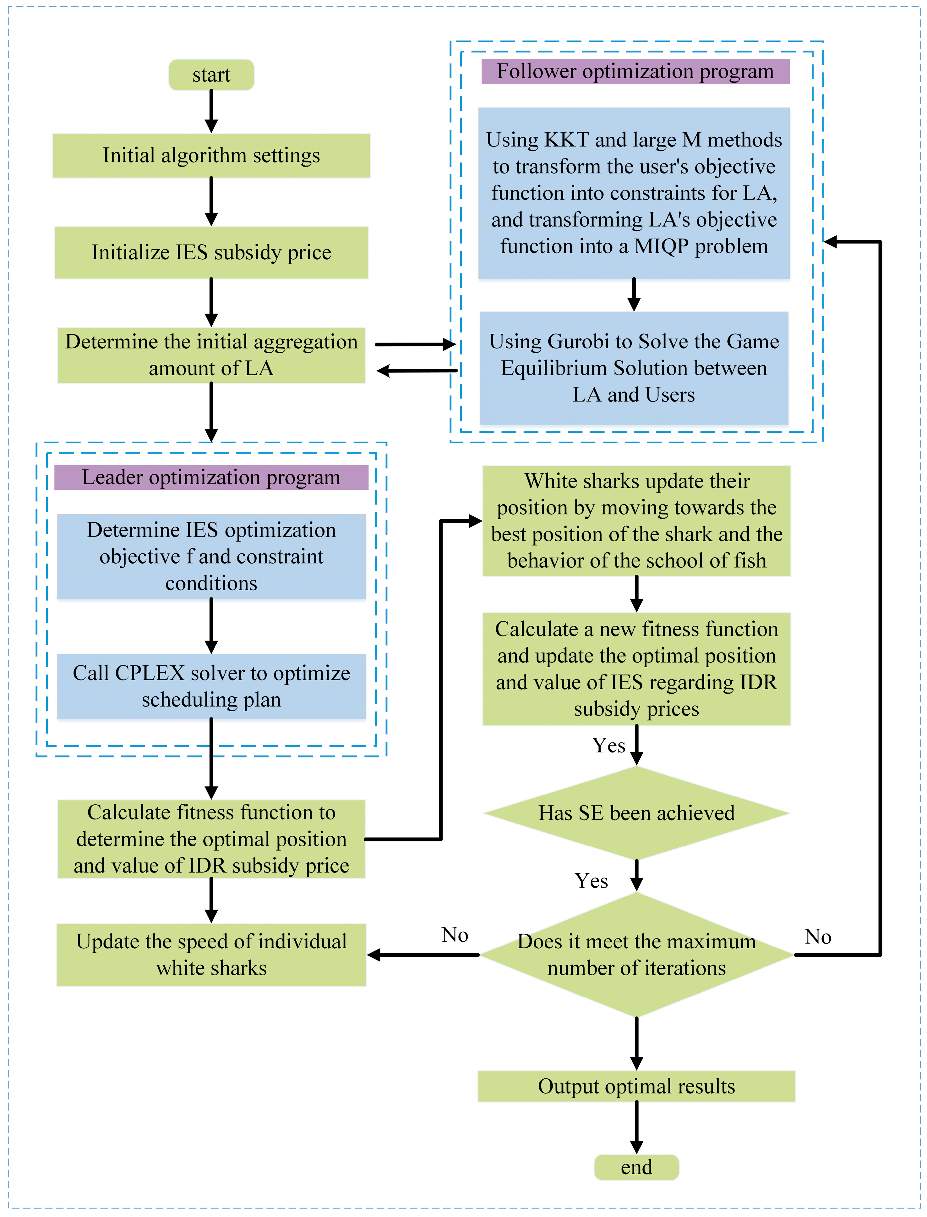
5. Solving Game Models

There are two common methods for solving traditional dual agent optimization problems: (1) using KKT transformation to transform the dual agent optimization problem into a single agent optimization problem [37] and (2) directly solving based on a distributed iterative algorithm [38]. This paper refers to the solution of the dual agent optimization problem. Firstly, the KKT condition and the Big M method are used to transform the user’s objective function into a constraint condition of LA, that is, the multi-agent two-level game model is transformed into a game problem between IES and LA. Secondly, the WSO algorithm and Gurobi solver are combined to solve the game equilibrium solution.

5.1. KKT Conversion

Using KKT conditions to transform the user’s objective function into the constraint conditions of LA, the Lagrangian function of LA is obtained:

$$L_k^{RU}=\left(k_1\rho +k_2\alpha \right)P_{j,k,t}^{RU}-{\displaystyle \frac{1}{2}}{\mu }_k{\theta }_k{P_{j,k,t}^{RU}}^2-{\mu }_k{v}_k{P}_{j,k,t}^{RU}+({\lambda }_{lb}(t)-{\lambda }_{ub}(t))P_{j,k,t}^{RU}$$

(46)

$${\displaystyle \frac{\partial L_{j,k}^{RU}}{P_{j,k,t}^{RU}}}=k_1\rho +k_2\alpha -{\mu }_k{\theta }_k{P}_{j,k,t}^{RU}-{\mu }_k{v}_k+{\lambda }_{j,lb}(t)-{\lambda }_{j,ub}(t)=0$$

(47)

$$0\le P_{j,k,t}^{RU}\perp {\lambda }_{j,lb}(t)\ge 0$$

(48)

$$0\le (P_{j,\max }^{RU}-P_{j,k,t}^{RU})\perp {\lambda }_{j,ub}(t)\ge 0$$

(49)

where $j\in \{e,h,g\}$ represents the type of load, and $e,h$ and $g$ represent electricity, heat, and gas, respectively. $L_{j,k}^{RU}$ is the Lagrangian function of the $k-th$ user. Equation (47) sets its first-order derivative with respect to $P_{j,k,t}^{RU}$ to 0, where ${\lambda }_{j,lb}(t),{\lambda }_{j,ub}(t)$ are bivariate. Equations (48) and (49) represent the KKT transformation of Equation (44).

5.2. Linear Transformation

Due to the complementary constraints of Equations (48) and (49) being nonlinear and the objective function in LA containing a bilinear term $c_{j,t}^{LA}{P}_{j,k,t}^{RU}$, it is difficult to solve the problem directly. Therefore, by using the Big M method, Equations (48) and (49) are transformed into the following mixed integer linear constraints:

$$0\le P_{j,k,t}^{RU}\le {\pi }_{j,t}^{lb}M$$

(50)

$$0\le {\lambda }_{j,t}^{\mathrm{l}b}\le (1-{\pi }_{j,t}^{lb})M$$

(51)

$$0\le P_{j,\max }^{RU}-P_{j,k,t}^{RU}\le {\pi }_{j,t}^{ub}M$$

(52)

$$0\le {\lambda }_{j,t}^{ub}\le (1-{\lambda }_{j,t}^{ub})M$$

(53)

where ${\pi }_{j,t}^{lb},{\pi }_{j,t}^{ub}$ is a 0–1 variable, and M is a sufficiently large positive number. Equations (50)–(53) are equivalent to Equations (48) and (49). In addition, using the dual variable in the KKT optimal condition in Equation (47), $c_{j,t}^{LA}{P}_{j,k,t}^{RU}$ will be transformed into a quadratic term, represented as follows:

$$c_{j,t}^{LA}{P}_{j,k,t}^{RU}={\mu }_k{\theta }_k{(P_{j,k,t}^{RU})}^2+({\lambda }_{j,ub}(t)-{\lambda }_{j,lb}(t)+{\mu }_k{v}_k)P_{j,k,t}^{RU}$$

(54)

where the objective function of LA can be expressed as a mixed integer quadratic programming (MIQP) problem, as shown in Equation (55):

$$\max F_{LA}={\displaystyle \sum _{t=1}^T{c}_{j,t}^{IES}{P}_{j,t}^{LA}}-{\displaystyle \sum _{t=1}^T{\displaystyle \sum _{k=1}^K{c}_{j,t}^{LA}{P}_{j,k,t}^{RU}}}={\displaystyle \sum _{t=1}^T{\displaystyle \sum _{k=1}^K{c}_{e,t}^{IES}}}{P}_{j,k,t}^{RU}-{\mu }_k{\theta }_k{(P_{j,k,t}^{RU})}^2-({\lambda }_{e,ub}(t)-{\lambda }_{e,lb}(t)+{\mu }_k{v}_k)P_{j,k,t}^{RU}$$

(55)

5.3. Solving Process

The fundamental idea behind WSO, which was first put up by Malik Braik et al. in 2022, was inspired by the way great white sharks hunt and track prey as well as their keen senses of smell, hearing, and fish behavior. The principle and solution process of WSO are detailed in reference [39] and will not be elaborated on in this paper. Due to the strong optimization ability and fast convergence speed of WSO, this paper uses WSO combined with the Gurobi solver to solve the game model. First, the subsidy price $c_{j,t}^{IES}$ of IES is randomly initialized and passed to LA, and then the Gurobi solver is called to solve the Stackelberg game between LA and users, that is, the MIQP problem shown in Equation (55), and the optimal load response $P_{j,k,t}^{RU}$ is determined. Next, the load response $P_{j,t}^{LA}$ aggregated by LA is returned to the upper fitness function, and the optimal subsidy price $c_{j,t}^{IES}$ is solved using the WSO algorithm. At the same time, the CPLEX solver is embedded to calculate the optimal output of each unit of IES. Due to the fact that the solution of the Stackelberg game model can be transformed into the solution of optimization problems [40], using Gurobi to solve the MIQP problem, the optimal solution obtained is the equilibrium solution of the game between LA and the user. When the optimal subsidy price $c_{j,t}^{IES}$ found by the upper layer WSO algorithm in adjacent generations is the same, it can be considered that the Stackelberg game between IES and LA has reached equilibrium. The algorithm flowchart can be seen in Appendix A Figure A1.

6. Example Analysis

6.1. Parameter Settings

This paper takes an IES in northern China as an example for numerical analysis. The operating parameters of the system are shown in Appendix A 

Table A1. System operating parameters.

Parameter	Value	Parameter	Value
${\eta }_{GT}$	0.35	$D(\mathrm{kg/kW})$	0.425
$Q_{CH4}(\mathrm{MJ}/{\mathrm{m}}^3)$	35	$a_{c{o}_2}$	0.55
$P_{\min }^{GT}/\mathrm{kW}$	50	$b_{c{o}_2}$	0.65
$P_{\min }^{GT}/\mathrm{kW}$	500	$c_{c{o}_2}$	18.20
$h_1$	0.15	$\lambda$	0.25
$h_2$	0.2	$l$	5
$h_m$	0.85	$\alpha$	0.25
${\eta }_{GB}$	0.9	$a(\mathrm{\$}/\mathrm{k}\mathrm{W})$	0.013
$\gamma$	0.55	$b(\mathrm{\$}/\mathrm{k}\mathrm{W})$	0.004
${\alpha }_{C02}(T/(\mathrm{M}\mathrm{W}\cdot \mathrm{h}))$	0.2	$c(\mathrm{\$}/\mathrm{k}\mathrm{W})$	0.039
${\eta }_{P2G}$	0.6	$z_1$	0.15
$e_{\alpha }$	0.96	$z_2$	0.2
$w_{\alpha }$	0.513	$m_1(\mathrm{\$}/\mathrm{k}\mathrm{W})$	0.15
${\eta }_{e,loss}$	0.02	$m_2(\mathrm{\$}/\mathrm{k}\mathrm{W})$	0.2
${\eta }_{h,loss}$	0.02	$k_t^C(\mathrm{\$}/\mathrm{t})$	9.8
$\eta$	0.95	$r^C(\mathrm{t}/(\mathrm{M}\mathrm{W}\cdot \mathrm{h}))$	0.76
$E_{e,\min }^{ES}/\mathrm{kW}$	50	${\mu }_k$	0.3
$E_{e,\max }^{ES}/\mathrm{kW}$	500	${\theta }_k$	0.02
$P_{e,\max }^{cha}/\mathrm{kW}$	100	${\nu }_k$	0.9
$P_{e,\max }^{dis}/\mathrm{kW}$	100	$P_{h,\max }^{cha}/\mathrm{kW}$	100
$E_{h,\min }^e/\mathrm{kW}$	50	$P_{h,\max }^{dis}/\mathrm{kW}$	100
$E_{h,\max }^{ES}/\mathrm{kW}$	500	$P_{\max }^{RU}$	150
$H^g(\mathrm{MJ}/{\mathrm{m}}^3)$	39

[23,34,41]. This paper considers that the fluctuation deviation of WT output is 10% of the predicted value, and the WT output curve is shown in Appendix A Figure A2 [42]. Reference [42] was used for purchase and sale electricity prices and natural gas prices in external markets. The subsidy price range for participating in IDR set by IES is [0.0983, 0.1683] USD/kWh, the subsidy price range for IDR set by LA is [0.0561, 0.0983] USD/kWh. The upper bound of the response of LA aggregated users is 10% of the benchmark load. The user baseline load curve is shown in Figure A2 [42], with attitudes ${\theta }_k$ and ${\nu }_k$ towards participating in demand response have values of 0.02 and 0.9, and the weight of discomfort cost ${\mu }_k$ is 0.4 [42]. In the WSO algorithm, the population size is set to 100, and the maximum number of iterations is 500. The simulation is modeled in the MATLAB R2018a compilation environment using the Cplex 12.10 optimization tool and solved based on the Gurobi solver.

6.2. Comparative Analysis of Economic and Environmental Benefits

To analyze the impact of IDR, ladder-type carbon trading mechanisms, and low-carbon technologies such as P2G and CCS on IES optimization scheduling, the following four scenarios are set up. In this section, the robustness coefficient of WT output is taken as an example in ${\mathrm{\Gamma }}_{WT}=6$. The cost of IES and the benefits of LA and users in different scenarios are shown in

Table 1. Comparison of IES costs and LA and user benefits in different scenarios.

Scenario	Total Cost/USD	CHP Cost/USD	Electricity Purchase Cost/USD	Gas Purchase Cost/USD	Carbon Trading Cost/USD	Carbon Emissions/kg	IDR Cost/USD	LA Benefits/USD	User Benefits/USD
1	4118.91	28.17	500.58	1863.28	1278.30	20,558.56	448.57	219.99	82.45
2	4174.54	66.26	274.75	1910.74	-	21,171.95	424.10	204.25	77.32
3	3950.52	21.87	541.11	1861.64	1087.11	17,857.54	438.78	168.74	59.50
4	3798.30	22.70	488.27	1768.65	1043.01	17,826.22	475.68	223.35	91.35

. Scenario 4 is the model established in this paper.

Scenario 1: without considering P2G and CCS devices, using the Stackelberg game to dynamically determine IDR subsidy prices.

Scenario 2: considering P2G and CCS devices, the objective function of IES does not include carbon trading costs and uses the Stackelberg game to dynamically determine IDR subsidy prices.

Scenario 3: considering P2G and CCS devices, a fixed IDR subsidy price is adopted, while the IES benchmark subsidy price is 0.8 CNY/kWh and the LA benchmark subsidy price is 0.55 CNY/kWh.

Scenario 4: considering P2G and CCS devices, the objective function of IES includes carbon trading costs and uses the Stackelberg game to dynamically determine IDR subsidy prices.

Compared with Scenario 1, the carbon emissions of the system in Scenario 4 decreased by 2732.34 kg, and the carbon trading cost decreased by USD 235.29. It can be seen that the introduction of P2G and CCS technology can achieve low-carbon operation of the system. At the same time, combined with Figure 4 and Figure 5, it can be seen that CCS technology can capture the carbon emissions of the system and react with P2G to synthesize natural gas, reducing the purchase cost of natural gas by USD 94.63. In addition, after the introduction of P2G and CCS technologies, the system needs to use more electricity to supply P2G and CCS devices, which increases the demand for demand response resources in the system. This leads to an increase of USD 3.36 and USD 8.90 in revenue for LA and users in Scenario 4, respectively, but the increase in revenue is relatively small.

Compared with Scenario 2, the carbon emissions in Scenario 4 decreased by 3345.73 kg, indicating that the ladder-type carbon trading mechanism can effectively reduce carbon dioxide emissions. Combining Figure 4 and Figure 5, it can be concluded that without considering the cost of ladder-type carbon trading, the amount of natural gas purchased in Scenario 2 is significantly higher than in Scenario 4 and burning a large amount of natural gas will lead to a significant increase in carbon emissions. In addition, when the energy supply of the system is mainly provided by CHP units and carbon emission costs are not considered, the demand for demand response resources in the system will decrease, leading to a decrease in the subsidy prices provided by IES, further reducing the user response amount of LA aggregation, resulting in a decrease of USD 19.10 and USD 14.02 in revenue for LA and users in Scenario 2, respectively.

Compared with Scenario 3, IES has the lowest total cost in Scenario 4. It can be seen that compared to a fixed IDR subsidy price, the dynamic game IDR price can better improve the profits of IES, LA, and users. Specifically, although the IDR subsidy cost increased by USD 36.90 after using the Stackelberg game to decide the subsidy price, combined with Figure 4 and Figure 5, it can be seen that the system’s electricity purchase cost, gas purchase cost, and carbon trading cost decreased by USD 52.85, USD 93.00, and USD 44.10, respectively, for a total cost reduction of USD 152.22. At the same time, the benefits for LA and users were also the highest, increasing by USD 54.61 and USD 31.85, respectively. This is because the subsidy price set by IES reflects the time value of DR resources. When the unit subsidy price obtained by LA increases, it can further incentivize LA to aggregate user response, and users can also receive higher subsidy prices, which increases the benefits for LA and users.

In summary, by comparing the total cost of IES and the benefits of LA and users in four scenarios, this paper introduces a ladder-type carbon trading mechanism and low-carbon technologies such as P2G and CCS to effectively reduce the total cost and carbon emissions of IES while using Stackelberg game decision making to subsidize IDR prices. At the same time, it improves the benefits of LA and users, demonstrating the effectiveness of the proposed solution.

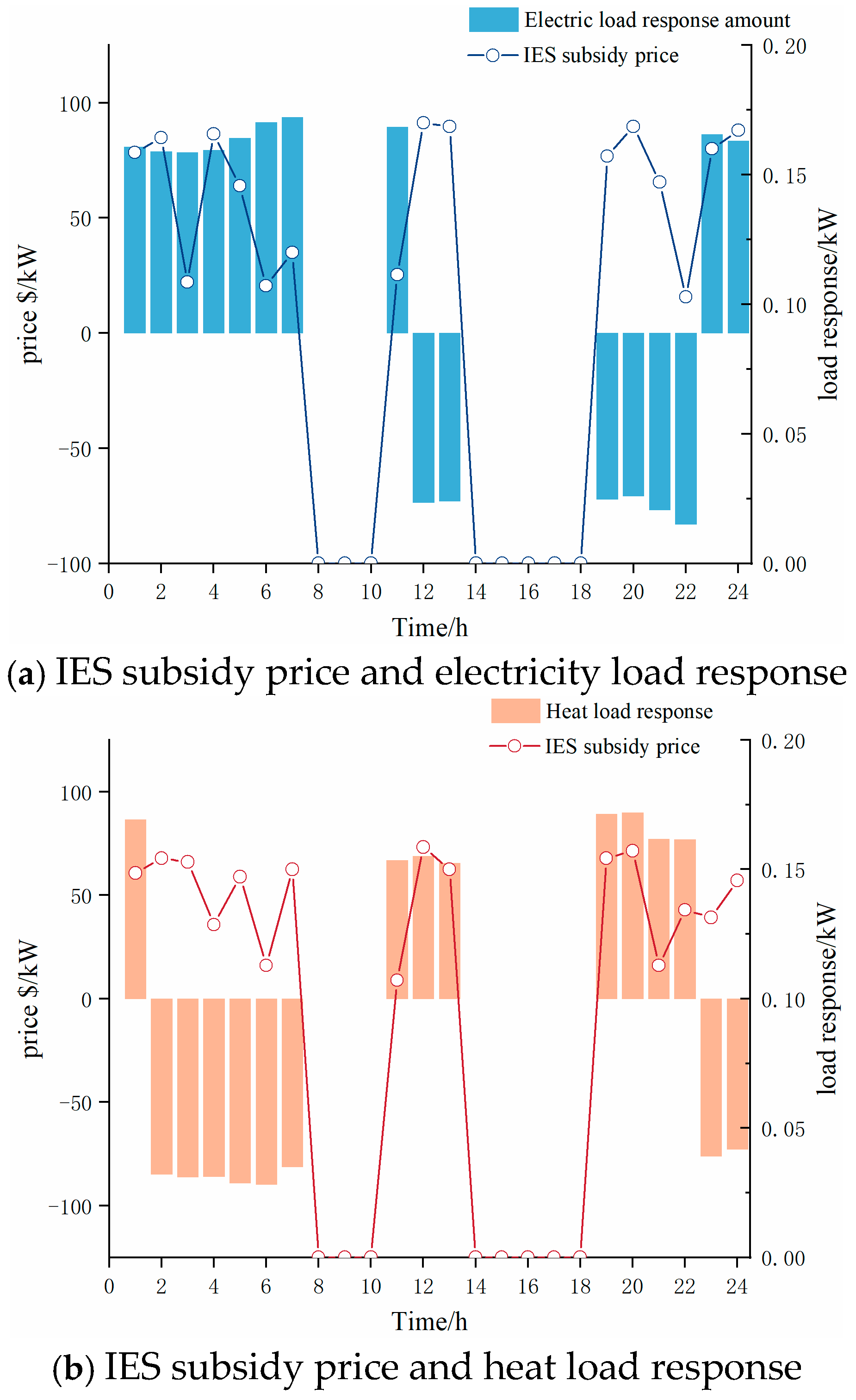
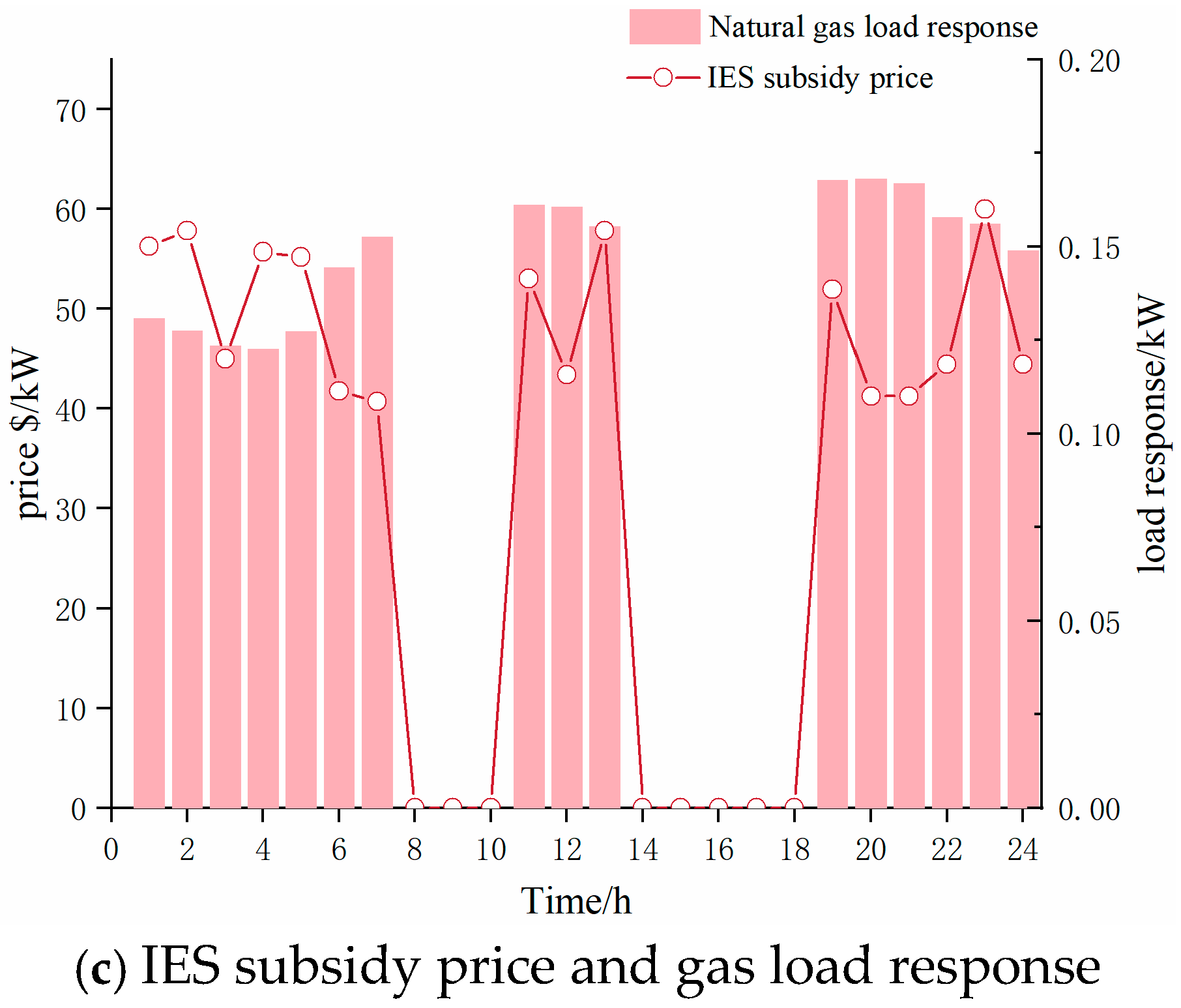
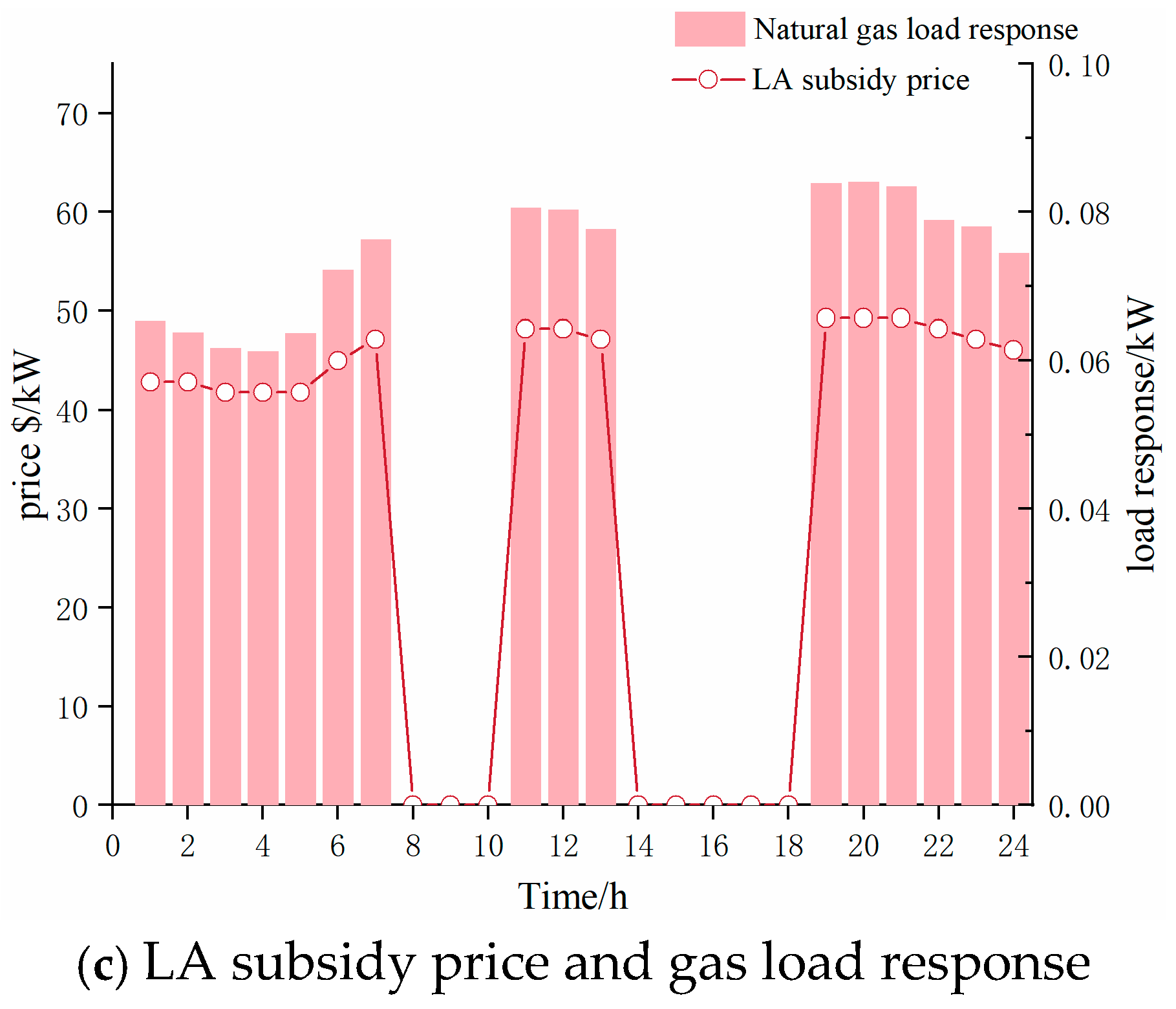
6.3. IDR Subsidy Prices and Response Amount

Based on the analysis of Scenario 4 in Section 6.2, in the game between IES and LA, the IDR subsidy prices provided by IES and the aggregated load response of LA are shown in Figure 6. It can be seen that IES incentivizes LA to aggregate load response during peak and low periods by dynamically adjusting subsidy prices. Specifically, the average subsidy prices for electric energy DR, heat energy DR, and natural gas DR during peak hours of 11–13 h and 19–23 h are 1.06 CNY/kWh, 1.01 CNY/kWh, and 0.87 CNY/kWh, respectively. The average subsidy prices for electric energy DR, heat energy DR, and natural gas DR during the low period of 1–7 h and 24 h are 1.01 CNY/kWh, 0.99 CNY/kWh, and 0.95 CNY/kWh, respectively.

In the game between LA and users, LA provides subsidy prices and user response quantities for users to participate in IDR, as shown in Figure 7. Taking electricity as an example, the load reduction provided by users during 6–7 h and 23–24 h is relatively large, and the average subsidy price obtained during this period is USD 0.082. Between 19–21 h, the amount of load transfer provided by users is relatively small, and the average subsidy price obtained during this period is USD 0.072. The subsidy price provided by LA to users for participating in IDR increases with the increase in user response amount.

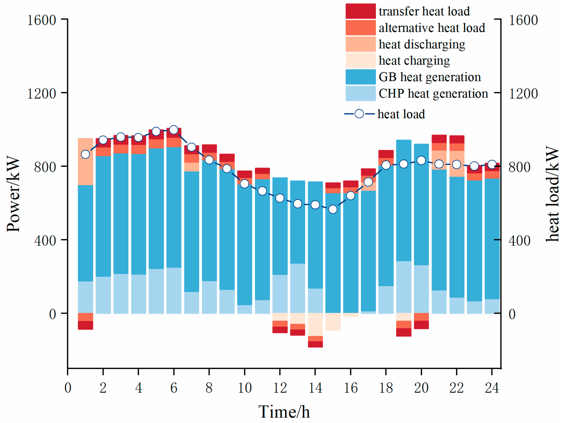
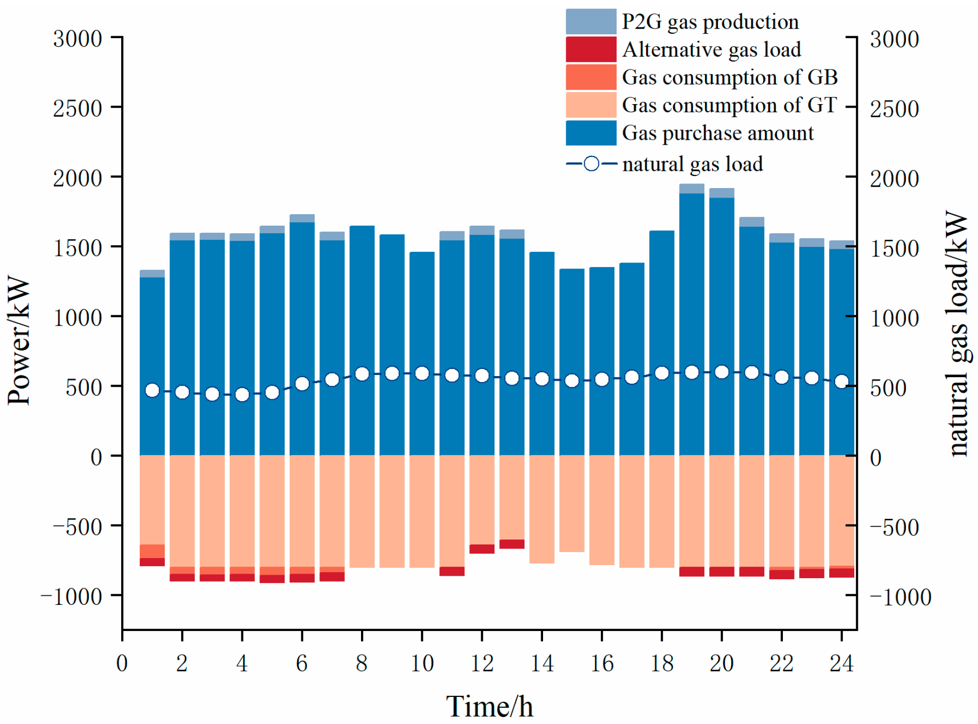
6.4. Scheduling Results

Based on the analysis of Scenario 4 in Section 6.2, the results of power scheduling optimization are shown in Figure 8. WT, CHP, garbage incineration devices, and electricity purchases are the main energy inputs. In order to absorb WT as much as possible on site, a portion of the daytime electricity demand is transferred to the nighttime. The results of heat energy scheduling optimization are shown in Figure 9, where the CHP unit provides a large amount of heat energy, and under the IDR mechanism, a portion of the heat load demand at night is transferred to the daytime period. In addition, due to the transfer of electricity load demand from daytime to nighttime, the output of CHP can be reduced, and the heat power demand can be supplied by a more efficient GB at this time. The results of natural gas scheduling optimization are shown in Figure 10. The system supplies GT and GB by burning natural gas, while P2G and CCS equipment can convert carbon dioxide into natural gas, reducing the purchase of natural gas in the system. In addition, during nighttime periods, the heat and gas loads of the system are replaced by electricity loads, making the electricity load demand curve as close as possible to the wind power curve. During the scheduling period, through the flexible cooperation of various internal equipment in the system, all wind power is consumed.

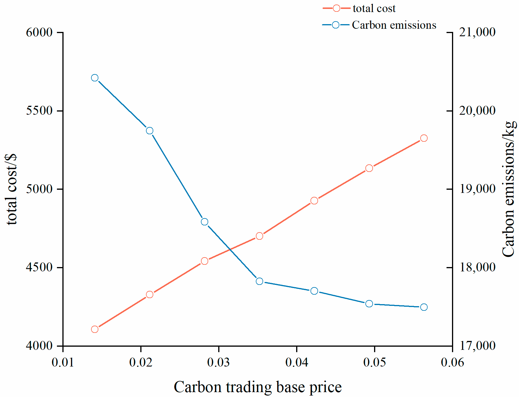
6.5. Sensitivity Analysis of Ladder-Type Carbon Trading Parameters

This section focuses on the impact of carbon trading base price and price growth rate on system operation. According to Appendix A 

Table A2. System costs under different carbon trading base prices.

Carbon Trading Base Price	IES Total Cost	Electricity Purchase Cost	Gas Purchase Cost	Carbon Trading Cost
0.1	3300.92	317.47	1897.33	503.47
0.15	3522.68	363.46	1881.43	726.78
0.2	3735.13	473.78	1846.14	903.66
0.25	3798.30	488.27	1768.65	1043.01
0.3	4119.60	557.69	1822.28	1281.18
0.35	4326.40	579.26	1817.22	1478.59
0.40	4517.19	584.36	1814.56	1685.03

and Figure 11, it can be seen that as the carbon trading base price increases, the cost of carbon trading gradually increases, leading to an increase in the total system cost. At this time, the system must reduce unit output to reduce its own carbon emissions. Therefore, the system’s electricity purchase cost gradually increases, while the gas purchase cost gradually decreases. When the carbon trading base price is greater than 0.035 USD/kg, the carbon emissions level of the system also tends to stabilize, basically maintaining around 17,000 kg. According to Appendix A 

Table A3. System costs under different carbon price growth rate.

Price Growth Rate	IES Total Cost	Electricity Purchase Cost	Gas Purchase Cost	Carbon Trading Cost
0.1	3705.63	393.83	1877.20	886.93
0.15	3791.90	474.07	1852.38	941.87
0.2	3873.94	523.42	1839.00	1002.64
0.25	3809.00	489.64	1773.63	1045.95
0.4	4159.84	583.29	1820.58	1322.42
0.6	4460.98	611.81	1813.47	1647.85
0.80	4775.20	659.72	1804.20	1945.57

and Figure 12, it can be seen that as the price growth rate increases, the carbon trading cost also increases. Therefore, the system reduces carbon emissions by increasing the purchase of electricity and IDR response while reducing the purchase of gas. When the price growth rate is greater than 0.4, the changes in equipment output and carbon emissions tend to stabilize, basically maintaining around 17,000 kg. In summary, reasonable adjustment of carbon trading base price and price growth rate can effectively control the total cost and carbon emissions of the system.

7. Conclusions

On the basis of the bilateral IDR trading mechanism, this paper establishes a multi-agent optimization scheduling model that includes IES, LA, and users. The model uses a two-level Stackelberg game to dynamically decide the IDR subsidy price. Meanwhile, a ladder-type carbon trading mechanism and low-carbon technologies such as P2G and CCS have been introduced within IES. The conclusions drawn from several case studies indicate the following:

(1) Compared with a fixed IDR subsidy price, this paper uses the Stackelberg game model to dynamically decide IDR subsidy prices, achieving significant economic benefits. Specifically, IES costs decreased by USD 152.22, while LA and user benefits increased by USD 54.61 and USD 31.85, respectively.

(2) The ladder-type carbon trading mechanism and low-carbon technology have effectively achieved low-carbon operation of the system. Specifically, after the introduction of a ladder-type carbon trading mechanism, IES carbon emissions decreased by 3345.73 kg. After adding CCS and P2G devices to conventional CHP units, carbon emissions decreased by 2732.34 kg and carbon trading costs decreased by USD 207.21.

(3) Considering the ladder-type carbon trading model, the total cost of IES increases with the increase in carbon trading base price and price growth rate, while the carbon emissions decrease with the increase in carbon trading base price and price growth rate and finally tend to a stable value. Under a certain carbon trading base price and price growth rate, a relative balance between carbon emission costs and maximum economic benefits can be achieved.

Overall, the scheduling strategy proposed in this paper can achieve higher economic benefits and provide some reference for the development of IES. This paper only considers trading between a single IES and LA. Further research can focus on energy trading between various IESs and LAs. Furthermore, this paper only considers the uncertainty of renewable energy output. In the future, load uncertainty can be included in research, and more applicable distributed robust optimization can be used to deal with uncertainty problems.

References

1. Liang, T.; Zhang, X.; Tan, J.; Jing, Y.; Lv, L. Deep reinforcement learning-based optimal scheduling of integrated energy systems for electricity, heat, and hydrogen storage. Electr. Power Syst. Res. 2024, 233, 110480. [Google Scholar] [CrossRef]
2. Wang, C.; Chen, S.; Zhao, J.; Zhou, Y.; Wei, Z.; Zheng, S. Coordinated scheduling of integrated electricity, heat, and hydrogen systems considering energy storage in heat and hydrogen pipelines. J. Energy Storage 2024, 85, 111034. [Google Scholar] [CrossRef]
3. Zhao, Z.; Liu, X. Flexible resource optimization allocation of park electric heating integrated energy system considering demand response. Mod. Electr. Power 2023, 1–11. [Google Scholar] [CrossRef]
4. Mo, J.; Yan, G.; Song, N.; Yuan, M. A review of research on optimization and scheduling of electric heating integrated energy systems based on demand response. Adv. Eng. Sci. 2023, 1–16. [Google Scholar] [CrossRef]
5. Nawaz, A.; Zhou, M.; Wu, J.; Long, C. A comprehensive review on energy management, demand response, and coordination schemes utilization in multi-microgrids network. Appl. Energy 2022, 323, 119596. [Google Scholar] [CrossRef]
6. Zhang, J.; Liu, Z. Low carbon economic scheduling model for a park integrated energy system considering integrated demand response, ladder-type carbon trading and fine utilization of hydrogen. Energy 2024, 290, 130311. [Google Scholar] [CrossRef]
7. Zhang, G.; Niu, Y.; Xie, T.; Zhang, K. Multi-level distributed demand response study for a multi-park integrated energy system. Energy Rep. 2023, 9, 2676–2689. [Google Scholar] [CrossRef]
8. Zhang, M.; Yang, J.; Yu, P.; Tinajero, G.D.; Guan, Y.; Yan, Q.; Zhang, X.; Guo, H. Dual-Stackelberg game-based trading in community integrated energy system considering uncertain demand response and carbon trading. Sustain. Cities Society 2024, 101, 105088. [Google Scholar] [CrossRef]
9. Tan, M.; Wang, L.; Jiang, C.; Liu, H.; Wu, L.; Tang, J. A Double Layer Optimization Model for Demand Response Considering the Adjustment Potential of Load Aggregators. Electr. Power 2022, 55, 32–44. [Google Scholar]
10. Jangid, B.; Mathuria, P.; Gupta, V. A hierarchical scheduling framework for DSO and shiftable load aggregator. Electr. Power Syst. Res. 2023, 225, 109861. [Google Scholar] [CrossRef]
11. Yan, H.; Hou, H.; Deng, M.; Si, L.; Wang, X.; Hu, E.; Zhou, R. Stackelberg game theory based model to guide users’ energy use behavior, with the consideration of flexible resources and consumer psychology, for an integrated energy system. Energy 2024, 288, 129806. [Google Scholar] [CrossRef]
12. Zhang, H.; Yang, Y.; Zhao, X.; Xu, N.; Li, C.; Xue, W. Dual layer optimization scheduling strategy for regional integrated energy systems considering demand response. Electr. Power 2021, 54, 141–150. [Google Scholar]
13. Li, Z.; Liu, Q.; Guo, W. Stackelberg Game Strategy Between Integrated Energy Microgrid Operators and Load Aggregators Considering Users Energy Consumption Behavior. South. Power Syst. Technol. 2022, 16, 35–46. [Google Scholar]
14. Najafi, A.; Jasiński, M.; Leonowicz, Z. A hybrid distributed framework for optimal coordination of electric vehicle aggregators problem. Energy 2022, 249, 123674. [Google Scholar] [CrossRef]
15. Wang, X.; Zhao, H.; Tan, Z. Optimization of dual layer master-slave game operation in comprehensive energy systems considering load aggregators. Renew. Energy Resour. 2023, 41, 1554–1562. [Google Scholar]
16. Li, S.; Zhang, L.; Nie, L.; Wang, J. Trading strategy and benefit optimization of load aggregators in integrated energy systems considering integrated demand response: A hierarchical Stackelberg game. Energy 2022, 249, 123678. [Google Scholar] [CrossRef]
17. Li, J.; Ai, Q.; Yin, S.; Hao, R. An aggregator-oriented hierarchical market mechanism for multi-type ancillary service provision based on the two-loop Stackelberg game. Appl. Energy 2022, 323, 119644. [Google Scholar] [CrossRef]
18. Soepyan, F.B.; Habib, M.; Zhang, Z.; Nemetz, L.R.; Haque, M.E.; Esquino, A.M.; Rivero, J.R.; Bhattacharyya, D.; Lipscomb, G.G.; Matuszewski, M.S.; et al. Optimization of a Natural Gas Power Plant with Membrane and Solid Sorbent Carbon Capture Systems. Carbon Capture Sci. Technol. 2024, 10, 100165. [Google Scholar] [CrossRef]
19. Park, J.; Kang, S.; Kim, S.; Kim, H.; Cho, H.S.; Lee, J.H. Enhancing the economic viability and reliability of renewables based electricity supply through Power-to-Gas-to-Power with green hydrogen. Energy Convers. Manag. 2024, 310, 118485. [Google Scholar] [CrossRef]
20. Chen, M.; Lu, H.; Chang, X.; Liao, H. An optimization on an integrated energy system of combined heat and power, carbon capture system and power to gas by considering flexible load. Energy 2023, 273, 127203. [Google Scholar] [CrossRef]
21. Liang, N.; He, X.; Tan, J.; Pan, Z.; Zheng, F. Stackelberg game-based optimal scheduling for multi-community integrated energy systems considering energy interaction and carbon trading. Int. J. Electr. Power Energy Syst. 2023, 153, 109360. [Google Scholar] [CrossRef]
22. Wang, L.; Zhang, Y.; Qu, Y. Optimization and scheduling of integrated energy systems for electricity to gas and carbon cycling based on a tiered carbon trading mechanism and refinement. Mod. Electr. Power 2023, 1–9, 335–343. [Google Scholar]
23. Chen, H.; Guo, S.; Song, X.; He, T. Design and evaluation of a municipal solid waste incineration power plant integrating with absorption heat pump. Energy 2024, 294, 131007. [Google Scholar] [CrossRef]
24. Chen, W.; Liu, Y.; Liu, W.; Zhang, X.; Wang, X. Two stage scheduling strategy for high-speed railway stations considering temperature control load in green electricity trading scenarios. Acta Energiae Solaris Sin. 2024, 1–10. [Google Scholar] [CrossRef]
25. Chen, Z.; Dong, Y.; Teng, M. Hybrid Generation of wind-solar-pumped storage thermal systems considering wind-solar uncertainties. China Rural Water Hydropower 2024, 08, 208–215. [Google Scholar]
26. Li, W.; Zou, Y.; Yang, H.; Fu, X.; Li, Z. Two stage stochastic Energy scheduling for multi energy rural microgrids with irrigation systems and biomass fermentation. IEEE Trans. Smart Grid, 2024; early access. [Google Scholar]
27. Dong, Y.; Zhang, H.; Ma, P.; Wang, C.; Zhou, X. A hybrid robust-interval optimization approach for integrated energy systems planning under uncertainties. Energy 2023, 274, 127267. [Google Scholar] [CrossRef]
28. Zhou, K.; Fei, Z.; Rong, H. Hybrid robust decentralized optimization of emission-aware multi-energy microgrids considering multiple uncertainties. Energy 2023, 265, 126405. [Google Scholar] [CrossRef]
29. Chen, Y.; Lu, X.; Zhang, H.; Zhao, C.; Xu, Y. Optimal configuration of integrated energy station using adaptive operation mode of combined heat and power units. Int. J. Electrical Power and Energy Systems 2023, 152, 109171. [Google Scholar] [CrossRef]
30. Ma, B.; Yang, L.; Chen, C.; Wang, Y.; Wang, B. Collaborative optimization strategy for integrated energy systems considering demand response. Renew. Energy Resour. 2023, 41, 676–684. [Google Scholar]
31. Wang, N.; Jin, Q.; Wang, S.; Gao, Y. A low-carbon co integration optimization model considering the combined operation of waste incineration power plants and electricity to gas conversion. Chin. J. Electr. Eng. 2023, 1–10. [Google Scholar]
32. Zheng, W.; Xu, Z.; Shao, Z.; Li, J.; Lei, K.; Li, J. Optimal dispatch of nearly-zero carbon integrated energy system considering waste incineration plant-carbon capture system and market mechanisms. Int. J. Hydrogen Energy 2023, 48, 27013–27031. [Google Scholar] [CrossRef]
33. Yan, N.; Li, X.; Wu, Z.; Shao, J.; Guerrero, J.M. Low-Carbon economic scheduling with Demand-Side response uncertainty in regional integrated energy system. Int. J. Electr. Power Energy Syst. 2024, 156, 109691. [Google Scholar] [CrossRef]
34. Luo, Z.; Wang, J.; Wang, H.; Zhao, W.; Yang, L. Optimization scheduling of integrated energy systems considering carbon capture and electricity to gas conversion. Electr. Power Autom. Equip. 2023, 43, 127–134. [Google Scholar]
35. Wu, Q.; Li, C. Economy-environment-energy benefit analysis for green hydrogen based integrated energy system operation under carbon trading with a robust optimization model. J. Energy Storage 2022, 55, 105560. [Google Scholar] [CrossRef]
36. Yu, M.; Hong, S.H. Incentive-based demand response considering hierarchical electricity market: A Stackelberg game approach. Appl. Energy 2017, 203, 267–279. [Google Scholar] [CrossRef]
37. Xu, Y.; Liu, H.; Sun, S.; Mi, L. Double layer optimization scheduling of multi microgrid systems considering demand response and shared energy storage. Electr. Power Autom. Equip. 2023, 43, 18–26. [Google Scholar]
38. Zhang, Y.; Zhao, H.; Li, B.; Wang, X. Research on dynamic pricing and operation optimization strategy of integrated energy system based on Stackelberg game. Int. J. Electr. Power Energy Syst. 2022, 143, 108446. [Google Scholar] [CrossRef]
39. Li, H.; Cui, S.; Fan, W. Low carbon economic scheduling of integrated energy systems based on improved white shark algorithm. Electr. Meas. Instrum. 2023, 6, 1–11. [Google Scholar]
40. Xie, C.; Wang, B.; Zhao, S.; Tan, J.; Huang, J.; Xie, Z. Solving Electricity Market Equilibrium Based on Double Layer Particle Swarm Optimization Algorithm. Power Syst. Technol. 2018, 42, 1170–1177. [Google Scholar]
41. Chen, J.; Hu, Z.; Chen, J.; Chen, Y.; Gao, M.; Lin, M. Optimization and scheduling of integrated energy systems considering stepped carbon trading and flexible supply-demand dual response. High Volt. Eng. 2021, 47, 3094–3106. [Google Scholar]
42. Liu, W.; Yao, Q.; Wang, Y.; Chen, L.; Lu, Y. A master-slave game power planning model based on a stepped demand response mechanism for supply and demand. Autom. Electr. Power Syst. 2022, 46, 54–63. [Google Scholar]
Figure 1. IES energy flow.
Energies 17 05491 g001
Figure 2. IES transaction architecture considering bilateral IDR.
Energies 17 05491 g002
Figure 3. Two-level Stackelberg game framework.
Energies 17 05491 g003
Figure 4. Electricity purchase curve under different scenarios.
Energies 17 05491 g004
Figure 5. Gas purchase curves under different scenarios.
Energies 17 05491 g005
Figure 6. IDR subsidy prices and load responses provided by IES.
Energies 17 05491 g006aEnergies 17 05491 g006b
Figure 7. IDR subsidy prices and load responses provided by LA.
Energies 17 05491 g007aEnergies 17 05491 g007b
Figure 8. Electricity scheduling result.
Energies 17 05491 g008
Figure 9. Heat scheduling result.
Energies 17 05491 g009
Figure 10. Natural gas scheduling result.
Energies 17 05491 g010
Figure 11. Analysis of carbon trading base price.
Energies 17 05491 g011
Figure 12. Analysis of price growth rate.
Energies 17 05491 g012