Abstract
This paper presents a proposal in which the maximum energy density criterion is used to evaluate the dynamic accuracy of LVDT (Linear variable differential transformer) sensors for applications in the energy industry. The solutions proposed in the paper are based on a mathematical model of the LVDT sensor, represented by its frequency response. The mathematical foundations required for the synthesis of such a model and the formulae and algorithm necessary to determine the maximum energy density for the integral-square error criterion are presented. Numerical and simulation calculations are performed using MathCad 15 and MATLAB R2014a programs. The solutions presented in this paper can constitute a basis for the selection of LVDT sensors for applications in the energy industry, with a view to achieving accurate diagnostic measurements.
1. Introduction
Linear variable differential transformer (LVDT) sensors are widely used in many branches of the energy industry, and particularly for measuring the linear motion and position of various types of elements (mainly actuators and valves) in power plants, for monitoring the condition of electrical machines and devices (for example, the condition of bearings and other moving elements), in industrial control and automation systems (automatic regulation systems), for optimizing energy processes and improving their reliability, and for diagnosing the position of energy elements in order to ensure operational safety and early detection of potential faults of energy machines and devices [1,2].
Compared to other sensors used for similar purposes (e.g., eddy current accelerometers), LVDT sensors are characterized by significant resistance to both mechanical and electromagnetic interference. They are therefore ideally suited for use in difficult environmental conditions, which undoubtedly occur in the energy industry. However, the measurement accuracy of these sensors is very important in many applications [2,3]. In engineering applications, this accuracy is assessed by calibration, which aims to determine the voltage sensitivity value and the relationship between the sensor output voltage and their core displacement [4]. Since these sensors process time-varying signals, their accuracy should be assessed on the basis of the relevant amplitude-frequency characteristics, which can be obtained by implementing frequency excitation in a practical measurement experiment and using appropriate control and measurement equipment (e.g., a function generator and oscilloscope or virtual measuring devices implemented in LabVIEW) [5]. Based on the measurement points of these characteristics, parametric identification of the sensor is performed, with the aim of determining the parameters of its mathematical model, represented by the relevant frequency response [6,7]. For this purpose, dedicated numerical methods such as the Monte Carlo method [8] or the Levenberg–Marquardt algorithm [9] should be used for regression of the measurement points of the amplitude-frequency characteristics. In this paper, we do not consider aspects related to the implementation of a practical measurement experiment aimed at determining the measurement points of the amplitude-frequency characteristics [10]. The frequency response is the basis for further numerical calculations aimed at determining the dynamic accuracy of LVDT sensors, as represented by the corresponding maximum energy density for the integral-square error criterion [11]. These calculations are based on the sensor’s impulse response, which is determined by the mathematical transformation of the frequency response [12]. It is also necessary to synthesize a mathematical model of the standard that is used as a reference for determining the energy density [11,13]. The energy density corresponds to the maximum value of the dynamic error and is determined based on the signal with two constraints, which is obtained by the method of simulation [13,14]. We consider three types of standards, represented by sixth-order low-pass analogue Butterworth, Bessel, and Chebyshev filters [15,16]. The choice of the type of standard is arbitrary, although it is important that the same standard is used for a given comparative series of sensors [13]. The results obtained for all three different types of standards were compared, and the most suitable standard for determining the maximum energy density was selected [11,14]. All calculations performed here based on the mathematical model of LVDT sensors constitute a new approach to assessing their dynamic accuracy. This assessment can be treated as an additional criterion in the selection of LVDT sensors for energy applications, especially those that require the highest degree of accuracy for performing diagnostic measurements [17]. In practical applications (in actual industry), LVDT sensors with lower dynamic error values should be considered more accurate (processing the dynamic signals more faithfully) than sensors with higher such error values.
Section 2 explains the mathematical basis for determining the frequency response for the LVDT sensors and gives the formulae underlying the determination of the maximum energy density for the integral-square error criterion. Section 3 presents the results of numerical and simulation calculations together with their analysis, while Section 4 summarizes the results.
2. Materials and Methods
Figure 1 shows the equivalent circuit for the LVDT sensor without inter-winding capacitance. This circuit consists of one primary winding, two secondary windings wound opposite to each other, and a ferromagnetic core that is movable in the direction [2].
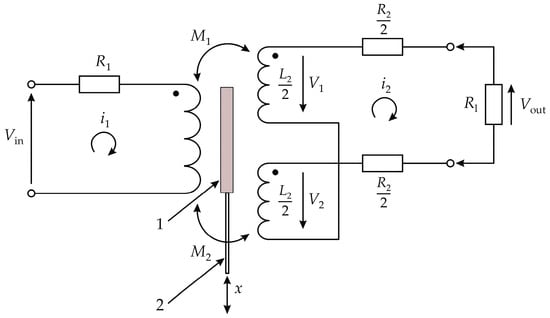
Figure 1.
Equivalent circuit for the LVDT sensor without inter-winding capacitance. —movable magnetic core, 2—core connecting rod, and —input and output voltages, and —voltages of the secondary circuits, and —mesh currents on the primary and secondary circuits, and —resistances of the primary and secondary circuits, —loaded resistance, and —self-inductances of the primary and secondary circuits, and —mutual inductances of the primary and secondary circuits.
The mathematical formulas for obtaining the frequency response of the LVDT sensor without inter-winding capacitance are derivated below.
The output voltage across the load resistor defined in the frequency domain is
where is the imaginary number and where denotes the frequency [Hz].
The secondary winding with no voltage source is defined by the following equation
where .
Deriving the current based on Equation (2) gives
An analysis of the primary circuit supplied with voltage gives
and then based on the transformation of formula Equation (4), we have
From a comparison of the right-hand sides of Equations (3) and (5), we have
where and , and is a constant value.
Substituting Equation (6) into Equation (1) gives
Dividing both sides of Equation (7) by we get
where denotes the frequency response of the LVDT sensor without inter-winding capacitance [2].
The integral-square error (ISE) is defined by the following equation:
where
and
while is is the translation parameter in the above convolution integral and denotes the time quantisation step.
The and in Equation (10) denote the impulse responses of the LVDT sensor and the corresponding reference, respectively [13,18,19,20].
Equation (11) defines the dynamic error as a function of time, while the integral-square error has the dimension of a numerical value, allowing for the comparison of dynamic errors of different types of sensors. The ISLE is the most popular quality factor used in broadly understood technology, hence it was used here as the evaluation index.
The impulse response is obtained by using the following transformation:
where denotes the inverse Fourier transformation [21].
The impulse response given in Equation (10) is calculated as follows:
where denotes the frequency response of the corresponding reference. The reference is selected in such a way that its frequency responses (amplitude and phase) meet the conditions of a non-distorting transformation [22,23]. According to the assumptions of this transformation, the amplitude response of the reference should have a constant value within the operating range of the LVDT sensor, while the phase response should have a linear shape within this range. These conditions can be met by analogue filters of the Butterworth, Bessel, or Chebyshev type [15,16].
The variable in Equation (9) denotes the input signal with two constraints, referring to the magnitude and the time of sensor testing. This signal is determined by simulation, in which the fixed-point algorithm [18,19] is implemented iteratively based on the initiating signal; this is determined on the basis of the transformation of the impulse response in Equation (10), as follows:
where denotes the signum function [24,25,26,27].
The maximum energy density is calculated with the following formula:
where is the complex conjugate of the wavelet used for the analysis, for which the wavelet is used, while and denote the scaling and translation factors, respectively [28,29].
The values of scaling and translation factors change during the subsequent steps of the wavelet transform, which allows determining the matching of the applied wavelet to the particular harmonics of the tested dynamic signal.
3. Results and Discussion
In actual industry, the accuracy of LVDT sensors is verified based on the calibration results of these sensors, performed using vibration calibrators, usually portable ones [30]. As a result of such calibration, the LVDT sensor gain factor is assessed based on the amplitude-frequency response. However, such an assessment does not reflect the dynamic error of such a sensor, which can only reliably reflect the dynamic accuracy of the considered sensor. Therefore, previously unpublished test results of the selected LVDT sensor are presented below.
The modeling results for an LVDT sensor of type DTA-10G8, represented by the values of the parameters of the frequency response given by Equation (8), are shown in Table 1. These are presented as a function of the core displacement x of the sensor. The sensor’s measurement range is 0–10 mm, the maximum linearity is equal to mm, the maximum repeatability of measurements is and its diameter is equal to 8 mm [31].

Table 1.
Parameters of the DTA-10G8 sensor.
The relationship of the gain factor to the core displacement over the range 0–10 mm was determined based on the modelling results presented in Table 1, where and denote the output and input voltages, respectively. This relationship was determined for a voltage of and an input voltage frequency of 1 kHz, and is presented in Figure 2. It should be noted that the central position of the sensor core is obtained for x = 0 mm.
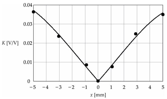
Figure 2.
Relationship between the gain factor and the core displacement.
Figure 2 confirms the linear relationship between the parameters and x for the DTA-10G8 sensor, over ranges from approximately −3 to 0 mm and from 0 to approximately 3 mm. Over the ranges from −5 mm to approximately −3 mm and from approximately 3 mm to 5 mm, this relationship is nonlinear.
Equation (16) shows the polynomial equation [32] that approximates the measurement points of the relationship shown in Figure 2 with minimum uncertainty in x and for the ranges (−5, 0) mm and (0, 5) mm.
where , and for the range (−5, 0) mm, and , and for the range (0, 5) mm. The approximation uncertainties are and for the two ranges, respectively. The uncertainties , and associated with the parameters , and are , , , for the range (−5, 0) mm, and , , , for the range (0, 5) mm, respectively.
Table 2.
Values of the parameter .
To determine the integral-square error given in Equation (9), it is necessary to determine the impulse responses and using Equations (11) and (12). The impulse response was determined for the parameters given in Table 1, while the impulse response was obtained based on the transfer functions for the Butterworth, Bessel, and Chebyshev filters, which are given by the following formulae:
and
where the filter ripple is equal to [15,16]. The parameter corresponds to the magnitude constraint on the input signal, which is obtained by simulation. For obvious reasons, the parameter has a value of , which is the value of the voltage . The parameter denotes the the filter cut-off frequency and corresponds to the frequency of the input voltage , which is equal to 1 kHz.
With considerable approximation, we can assume symmetry of the characteristic shown in Figure 2 with respect to the parameter x equal to 0 mm; hence, only the results in Table 1 were used for further calculations for x over the range (0, 5) mm.
Table 3 lists the calculation results for the ISE given by Equation (9) for four positions of the sensor core and for the three types of standard given in Equations (17)–(19).
Table 3.
Calculation results for the ISE.
The values of the cut-off frequency were determined based on 10% deviation of the amplitude-frequency response from the value corresponding to . An example of determining this deviation for x equal to 3 mm is shown in Figure 3.
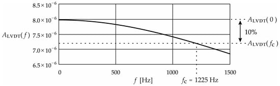
Figure 3.
Example illustrating the determination of the cut-off frequency .
The results in Table 3 indicate that the lowest values of the ISE were obtained when the Bessel filter was used as a reference, while the highest values were obtained for the Chebyshev filter. This means that the most accurate match between the impulse response of the considered LVDT sensor and the impulse response of the standard is obtained for the Bessel filter. The results therefore indicate that when carrying out accuracy tests of LVDT sensors, it is advisable to use the Bessel filters as a standard to determine the ISE. The lowest value of the ISE of the Bessel filter in Table 3 is probably due to the shape of the amplitude response obtained for this filter.
Figure 4 shows the impulse responses , and given in Equations (10)–(13) for the Bessel filter represented in Equation (19) for x = 3 mm, as an example.
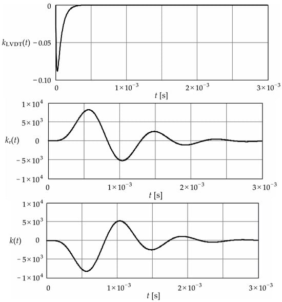
Figure 4.
Impulse responses and .
The impulse response has the property of a single-magnitude function with a negative value, and quickly converges (after about 0.2 ms) to zero. The impulse responses and were determined using Equations (12) and (10), respectively, and show that the signals have the property of changing slowly. The impulse is the basis for determining the ISE using Equation (9).
Figure 5 shows the shape of the signal obtained for the Bessel filter and for x = 3 mm based on Equation (14). This signal has a rectangular shape, with five switching events resulting from the zero crossing of the impulse response .
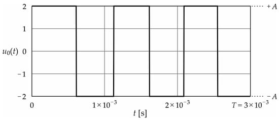
Figure 5.
Signal .
The signal shown in Figure 5 has the property that any other signal contained within its constraints can produce an ISE less than or at most equal to that signal [13]. The signal is therefore the worst case for the signal with two constraints, and , at the LVDT sensor input, in the sense that it gives the highest possible value of the ISE that can be obtained for this number of constraints and for the given numerical values.
Figure 6 shows the dynamic error , which enables the ISE to be calculated by using Equation (9). This error was obtained for the Bessel filter and x = 3 mm.
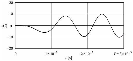
Figure 6.
Dynamic error .
The error exhibits the properties of a signal with gradually increasing oscillations and has four zero crossings.
The impulse responses , and shown in Figure 4, the signal presented in Figure 5, and the error shown in Figure 6 were generated using MathCad 15 program.
Figure 7 shows the energy density and normalized amplitude obtained for the signal presented in Figure 5, using MATLAB program. This energy density satisfies Equation (15) using the Morlet wavelet [33]. The signal is defined as ‘Analyzed Signal’ in this Figure 7. Below this signal, the relationship between Energy distribution and the frequency and time is given as a result of implementing the wavelet transform.
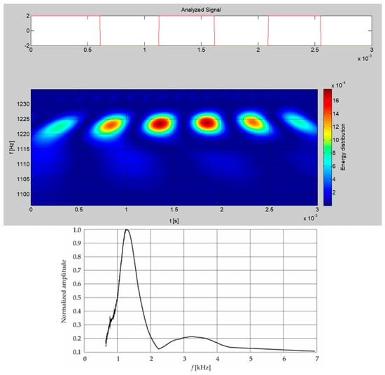
Figure 7.
Energy density of the signal .
The energy density and normalized amplitude shown in Figure 7 indicate that the strongly dominant frequency in the signal corresponds to the frequency response band of the LVDT sensor. Hence, to evaluate the accuracy of the LVDT sensor, modelled without inter-winding capacitance, an analysis of both the energy density and the normalized amplitude can be used. The signal that contains a dominant frequency component with a value close to the frequency range of the sensor can be considered to produce the maximum value of the ISE. Of course, the exact value of this error can be determined using Equation (9). The analysis presented in Figure 7 and the corresponding conclusions were confirmed for the remaining three core shifts and for the Butterworth and Chebyshev filters (according to the data in Table 3).
4. Conclusions
This paper has presented a method for assessing the accuracy of the LVDT sensors used in the power industry by determining the maximum value of the dynamic error according to the ISE criterion and by analyzing the energy density of the signal that produces this maximum error value. The results of the tests conducted here indicate that the best results were obtained for the Bessel filter, meaning that this type of filter is suitable for accuracy tests of LVDT sensors. The best match between the sensor impulse response and the standard impulse response is obtained with this filter. The ISE values obtained for the Butterworth and Chebyshev filters were 2.2 and 5.5 times higher, respectively, than for the Bessel filter. Using the research procedure described here, it is very important to use simulation to determine the worst-case scenario of the sensor input signal for which the highest value of the ISE and the corresponding energy density are obtained. The research methodology developed in this paper may be of great importance for both the selection and diagnostics of LVDT sensors for the energy industry, where the accuracy assessment of the sensors used is extremely important. It can also be used to study the optimization parameters of the mathematical standard for an LVDT sensor for the purpose of minimizing the value of the dynamic error resulting from the processing of dynamic signals by the sensor.
Author Contributions
Conceptualization, K.T.; methodology, K.T.; software, K.T.; validation, K.T., P.B. and K.O.; formal analysis, K.T., P.B. and K.O.; investigation, K.T.; resources, K.T.; data curation, K.T.; writing—original draft preparation, K.T.; writing—review and editing, K.T.; visualization, K.T.; supervision, K.T.; project administration, K.T.; funding acquisition, K.T. All authors have read and agreed to the published version of the manuscript.
Funding
This research was conducted at the Faculty of Electrical and Computer Engineering, Krakow University of Technology, and was financially supported by the Ministry of Science and Higher Education, Republic of Poland (grant no. E-1/2023).
Data Availability Statement
The original contributions presented in the study are included in the article, further inquiries can be directed to the corresponding author.
Conflicts of Interest
The authors declare no conflicts of interest.
References
- Jefriyanto, W.; Saka, B.G.M.; Pineng, M.; Djamal, M. Development of LVDT (Linear Variable Differential Transformer) sensor as land displacement sensor. J. Phys. Conf. Ser. 2020, 1528, 012041. [Google Scholar] [CrossRef]
- Tomczyk, K. Uncertainties in determining the upper bound of dynamic error for the LVDT sensor. Measurement 2024, 235, 114950. [Google Scholar] [CrossRef]
- Masi, A.; Danzeca, S.; Losito, R.; Peronnard, P.; Secondo, R.; Spiezia, G. A high precision radiation-tolerant LVDT conditioning module. Nucl. Instrum. Meth. A 2014, 745, 73–81. [Google Scholar] [CrossRef]
- Petchmaneelumka, W.; Songsuwankit, K.; Riewruja, V. Accurate LVDT signal converter. Int. J. Electr. Eng. 2016, 11, 340–347. [Google Scholar] [CrossRef]
- Wang, Y.; Egner, F.S.; Willems, T.; Naets, F.; Kirchner, M. Using multi-sine excitation and rigid body motion compensation in randomly sampled camera-based experimental modal analysis to improve SNR. Mech. Syst. Signal Process. 2023, 204, 110763. [Google Scholar] [CrossRef]
- Oliva-Gonzalez, L.J.; Martínez-Guerra, R. State estimation-based parameter identification for a class of nonlinear fractional-order systems. Nonlinear Dyn. 2024, 112, 6379–6402. [Google Scholar] [CrossRef]
- Xiao, F.; Zhu, W.; Meng, X.; Chen, G.S. Parameter Identification of Structures with Different Connections Using Static Responses. Appl. Sci. 2022, 12, 5896. [Google Scholar] [CrossRef]
- Kurtulbaş, E.; Ciğeroğlu, Z.; Şahin, S.; El Messaoudi, N.; Mehmeti, V. Monte Carlo, molecular dynamic, and experimental studies of the removal of malachite green using g-C3N4/ZnO/Chitosan nanocomposite in the presence of a deep eutectic solvent. Int. J. Biol. Macromol. 2024, 274, 133378. [Google Scholar] [CrossRef]
- Rubio, J.d.J. Stability Analysis of the Modified Levenberg–Marquardt Algorithm for the Artificial Neural Network Training. IEEE Trans. Neural Netw. Learn. Syst. 2020, 32, 3510–3524. [Google Scholar] [CrossRef]
- Božić, D.; Runje, B.; Razumić, A. Risk Assessment for Linear Regression Models in Metrology. Appl. Sci. 2024, 14, 2605. [Google Scholar] [CrossRef]
- Tomczyk, K.; Layer, E. Energy density for signals maximizing the integral-square error. Measurement 2016, 90, 224–232. [Google Scholar] [CrossRef]
- Yang, H.; Jing, X.; Yin, Z.; Chen, S.; Wang, C. A Method to Obtain the Transducers Impulse Response (TIR) in Photoacoustic Imaging. Appl. Sci. 2024, 14, 920. [Google Scholar] [CrossRef]
- Layer, E. Modelling of Simplified Dynamical Systems; Springer: Berlin/Heidelberg, Germany, 2002; ISBN 978-3-540-43762-8. [Google Scholar]
- Tomczyk, K. Monte Carlo-Based Procedure for Determining the Maximum Energy at the Output of Accelerometers. Energies 2020, 13, 1552. [Google Scholar] [CrossRef]
- Beşkirli, M.; Kiran, M.S. Optimization of Butterworth and Bessel Filter Parameters with Improved Tree-Seed Algorithm. Biomimetics 2023, 8, 540. [Google Scholar] [CrossRef] [PubMed]
- Mei, A. The Design and Simulation of a Fifth-order Chebyshev Low-Pass Filter. J. Phys. Conf. Ser. 2022, 2386, 012066. [Google Scholar] [CrossRef]
- Nikitin, Y.; Božek, P.; Peterka, J. Logical–Linguistic Model of Diagnostics of Electric Drives with Sensors Support. Sensors 2020, 20, 4429. [Google Scholar] [CrossRef]
- Honig, M.; Steiglitz, K. Maximizing the output energy of a linear channel with a time- and amplitude-limited input. IEEE Trans. Inf. Theory 1992, 38, 1041–1052. [Google Scholar] [CrossRef][Green Version]
- Elia, M.; Taricco, G.; Viterbo, E. Optimal energy transfer in band-limited communication channels. IEEE Trans. Inf. Theory 1999, 45, 2020–2029. [Google Scholar] [CrossRef][Green Version]
- Tomczyk, K.; Kowalczyk, M. Accuracy Assessment of Charge-Mode Accelerometers Using Multivariate Regression of the Upper Bound of the Dynamic Error. Energies 2023, 16, 7784. [Google Scholar] [CrossRef]
- Huang, J.; Glæsner, N.; Triolo, J.M.; Bekiaris, G.; Bruun, S.; Liu, F. Application of Fourier transform mid-infrared photoacoustic spectroscopy for rapid assessment of phosphorus availability in digestates and digestate-amended. Sci. Total Environ. 2022, 832, 155040. [Google Scholar] [CrossRef]
- Kumar, B.; Bag, S. Phase transformation effect in distortion and residual stress of thin-sheet laser welded Ti-alloy. Opt. Lasers Eng. 2019, 122, 209–224. [Google Scholar] [CrossRef]
- Wu, R.-C.; Huang, L.-J. Non-Distorted Optimization Spectrum Analysis. Energies 2018, 11, 1841. [Google Scholar] [CrossRef]
- Dichev, D.; Koev, H.; Bakalova, T.; Louda, P. A Model of the Dynamic Error as a Measurement Result of Instruments Defining the Parameters of Moving Objects. Meas. Sci. Rev. 2014, 14, 183–189. [Google Scholar] [CrossRef]
- Dichev, D.; Diakov, D.; Zhelezarov, I.; Valkov, S.; Ormanova, M.; Dicheva, R.; Kupriyanov, O. A Method for Correction of Dynamic Errors When Measuring Flat Surfaces. Sensors 2024, 24, 5154. [Google Scholar] [CrossRef] [PubMed]
- Tomczyk, K.; Beńko, P. Analysis of the Upper Bound of Dynamic Error Obtained during Temperature Measurements. Energies 2022, 15, 7300. [Google Scholar] [CrossRef]
- Dudzik, M.; Tomczyk, K.; Jagiello, A.S. Analysis of the error generated by the voltage output accelerometer using the optimal structure of an artificial neural network. In Proceedings of the 2018 19th International Conference on Research and Education in Mechatronics, REM 2018, Delft, The Netherlands, 7–8 June 2018. [Google Scholar] [CrossRef]
- Bialasiewicz, J.T. Wavelet-based approach to evaluation of signal integrity. IEEE Trans. Ind. Electron. 2013, 60, 4590–4598. [Google Scholar] [CrossRef]
- Huang, M.-C. Wave parameters and functions in wavelet analysis. Ocean Eng. 2004, 31, 111–125. [Google Scholar] [CrossRef]
- Datasheet for Portable Calibrator; 9110D Series; The Modal Shop: Cincinnati, OH, USA, 2023; Available online: https://www.modalshop.com/docs/themodalshoplibraries/datasheets/9110d-portable-vibration-calibrator-datasheet-ds-0103.pdf?sfvrsn=202f7b45_7 (accessed on 22 October 2024).
- Datasheet of the LVDT Sensor; DTA-xG8; Micro Epsilon: Birkenhead, UK; Available online: http://www.micro-epsilon.pl/download/indusensor-lvdt_dta_g8.pdf (accessed on 10 September 2024).
- Ostertagová, E. Modelling using Polynomial Regression. Procedia Eng. 2012, 48, 500–506. [Google Scholar] [CrossRef]
- Kumar, N.; Kumar, R. Wavelet transform-based multipitch estimation in polyphonic music. Heliyon 2020, 6, e03243. [Google Scholar] [CrossRef]


Disclaimer/Publisher’s Note: The statements, opinions and data contained in all publications are solely those of the individual author(s) and contributor(s) and not of MDPI and/or the editor(s). MDPI and/or the editor(s) disclaim responsibility for any injury to people or property resulting from any ideas, methods, instructions or products referred to in the content. |
© 2024 by the authors. Licensee MDPI, Basel, Switzerland. This article is an open access article distributed under the terms and conditions of the Creative Commons Attribution (CC BY) license (https://creativecommons.org/licenses/by/4.0/).