
An Open-Source Julia Package for RMS Time-Domain Simulations of Power Systems


Abstract
1. Introduction
- Simplification of the process of performing RMS simulations on power system models developed using the PowerModels.jl ecosystem;
- A flexible modeling framework that allows for the inclusion of a wide range of power system components and disturbances;
- Pre-constructed models of common power system components, such as synchronous generators, loads, and common generator control systems, that can be used to build models of power systems;
- A simple, easy-to-understand programming interface that is suitable for power system education.
2. RMSPowerSims.jl
2.1. High-Level Package Structure
| Algorithm 1 Power system equations. |
|
| Listing 1. Simulated dirtree within listing. | ||||
| 1 | PowerSystemSimulation | |||
| 2 | |-- | PowerSystemModel | ||
| 3 | | | |-- | Component List | |
| 4 | | | | | |-- | ComponentModel 1 & Pointers |
| 5 | | | | | |-- | ComponentModel 2 & Pointers |
| 6 | | | | | |-- | ... |
| 7 | | | | | ‘-- | ComponentModel n & Pointers |
| 8 | | | ‘-- | List of State & Algebraic Variables | |
| 9 | |-- | Initial Conditions | ||
| 10 | ‘-- | Disturbances | ||
| 11 | |-- | Disturbance 1 | ||
| 12 | |-- | Disturbance 2 | ||
| 13 | |-- | ... | ||
| 14 | ‘-- | Disturbance n | ||
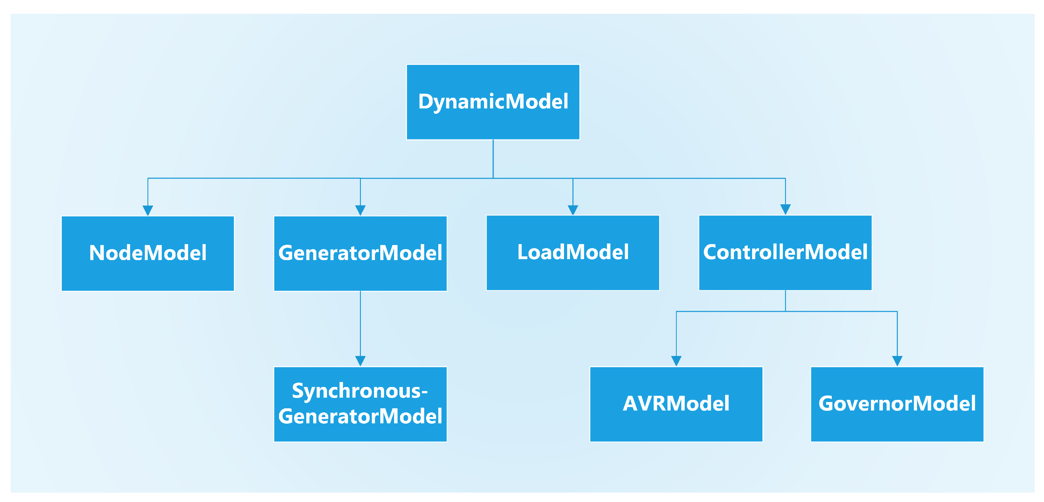
2.2. Component Models and Typing
- i is the index of the bus for which the power balance is being calculated;
- j is the index for generators connected to bus i;
- l is the index for loads connected to bus i;
- k is the index for summation over all buses in the network;
- is the set of generators connected to bus i;
- is the set of loads connected to bus i;
- is the set of buses in the network with branches connecting to bus i;
- are the voltage magnitudes at buses i and k, respectively;
- are the voltage phase angles at buses i and k, respectively;
- are the real and reactive power injections of generator j;
- are the real and reactive power demands of load l;
- is the magnitude of the admittance between buses i and k;
- is the phase angle of the admittance between buses i and k.
2.3. Implemented Component Models
2.4. Disturbances
- The values of state variables do not change from the time of the disturbance to the time immediately following the disturbance.
- The values of algebraic variables are allowed to change instantaneously.
- The values of the derivatives of the state variables are allowed to change instantaneously.
2.5. Package Functionality
- The package provides a modeling framework that extends the PowerModels.jl NDD format to incorporate additional parameters required for dynamic simulation.
- Hierarchical typing allows for the definition of custom models of power system components and their incorporation into the simulation.
- The package provides functionality to calculate the initial conditions for dynamic simulations.
- The package provides functionality to execute RMS time-domain simulations.
- The package provides the ability to recalculate the system state following a disturbance that causes a significant discontinuity in the system state variables. This is necessary for some disturbances which result in significant non-linearity in the system equations.
- The package provides functionality to visualize the results of simulations using the Plots.jl package.
3. Simulation Process
| Listing 2. Example of running a simulation using RMSPowerSims.jl. | |
| 1 | # Load network model |
| 2 | load_model("example_network") |
| 3 | |
| 4 | # Build PowerSystemSimulation object |
| 5 | power_system_simulation = prepare_simulation(net) |
| 6 | |
| 7 | # Set disturbances |
| 8 | faulted_bus_index = 3 |
| 9 | (t_fault, t_clear) = (0.5, 0.55) |
| 10 | power_system_simulation.disturbances = Disturbance[ |
| 11 | BusFault(faulted_bus_index, t_fault), |
| 12 | ClearBusFault(faulted_bus_index, t_clear, restart_simulation=true), |
| 13 | ] |
| 14 | |
| 15 | # Run simulation |
| 16 | tspan = (0.0, 10.0) |
| 17 | soln = run_RMS_simulation( |
| 18 | power_system_simulation, |
| 19 | tspan; |
| 20 | solver_settings=Dict( |
| 21 | "reltol" => 1e-9, |
| 22 | "abstol" => 1e-8, |
| 23 | "maxiters" => 10000, |
| 24 | "dtmax" => 0.01, |
| 25 | ) |
| 26 | ) |
| 27 | |
| 28 | # Add simulation results to network model |
| 29 | add_simulation_results!(net, soln) |
| 30 | |
| 31 | # Plot results |
| 32 | plot_res(net, "gen", 1, "Pg") |
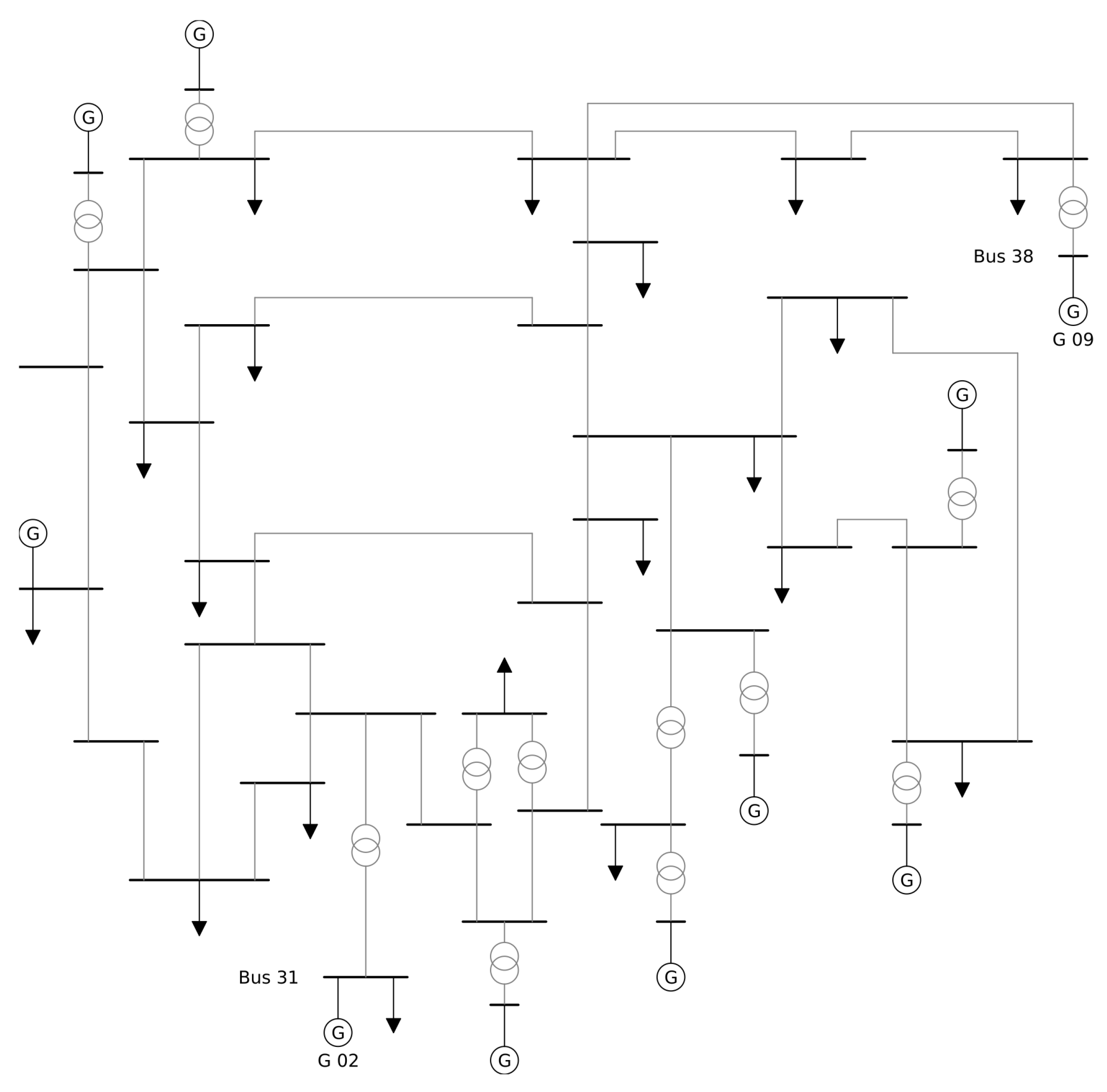
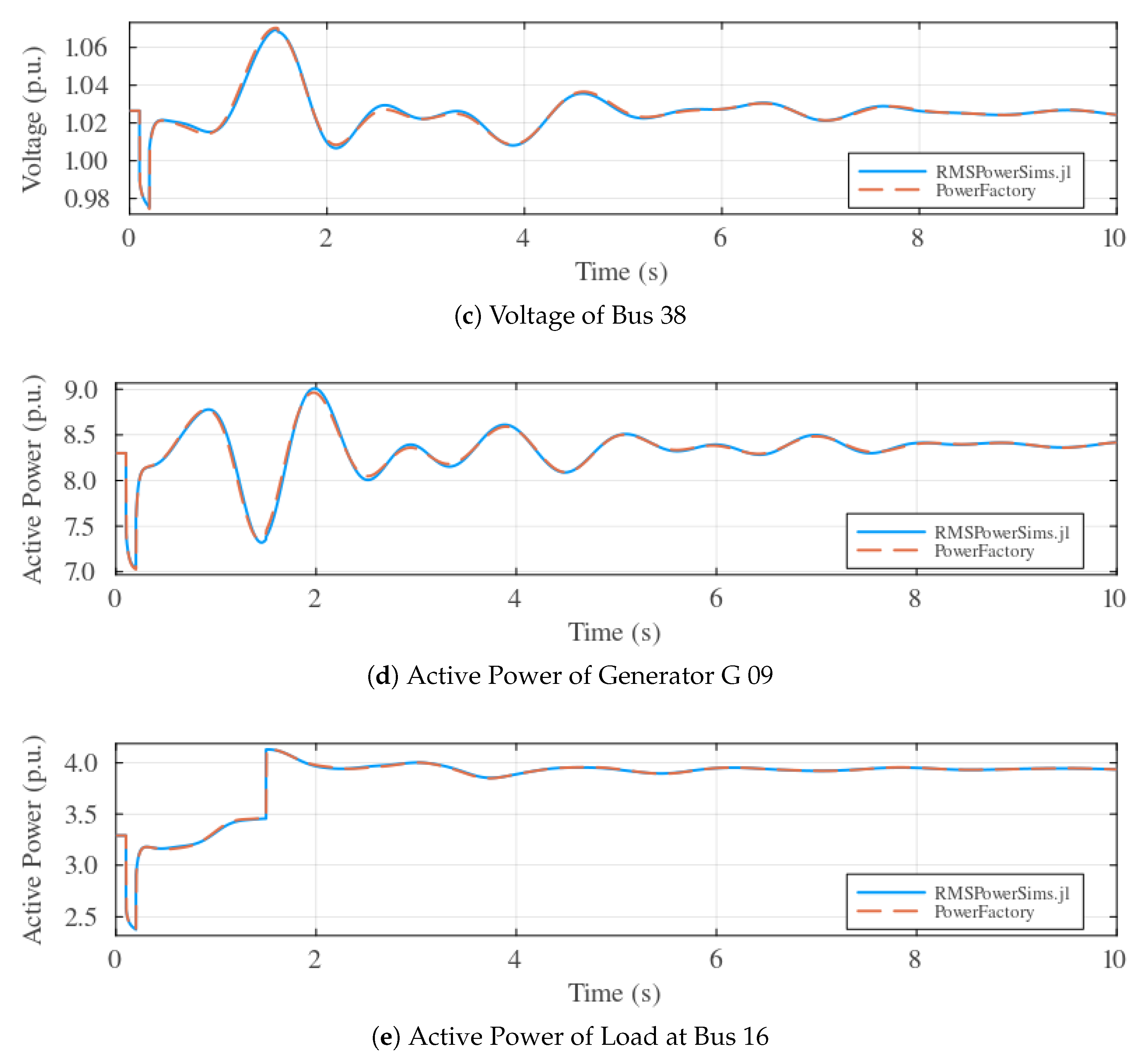
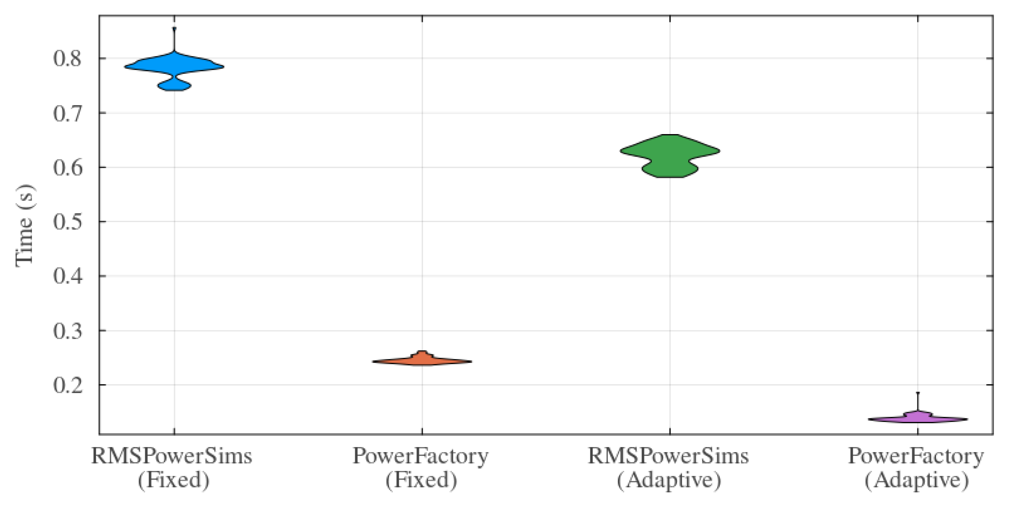
4. Verification
5. Conclusions
Author Contributions
Funding
Data Availability Statement
Conflicts of Interest
Abbreviations
| AC | Alternating Current |
| AVR | Automatic Voltage Regulator |
| DAE | Differential-Algebraic Equation |
| EMT | Electromagnetic Transient |
| IBG | Inverter-Based Generation |
| NDD | Network Data Dictionary |
| OPF | Optimal Power Flow |
| REG | Renewable Energy Generation |
| RMS | Root Mean Square |
Appendix A

| Name | Base Voltage (kV) | Bus Type | Voltage Magnitude (p.u.) | Voltage Angle (deg) |
|---|---|---|---|---|
| Bus 01 | 345.0 | PQ | 1.047 | −8.439 |
| Bus 02 | 345.0 | PQ | 1.049 | −5.754 |
| Bus 03 | 345.0 | PQ | 1.030 | −8.599 |
| Bus 04 | 345.0 | PQ | 1.004 | −9.607 |
| Bus 05 | 345.0 | PQ | 1.005 | −8.612 |
| Bus 06 | 345.0 | PQ | 1.008 | −7.950 |
| Bus 07 | 345.0 | PQ | 0.997 | −10.124 |
| Bus 08 | 345.0 | PQ | 0.996 | −10.615 |
| Bus 09 | 345.0 | PQ | 1.028 | −10.322 |
| Bus 10 | 345.0 | PQ | 1.017 | −5.427 |
| Bus 11 | 345.0 | PQ | 1.013 | −6.284 |
| Bus 12 | 138.0 | PQ | 1.000 | −6.244 |
| Bus 13 | 345.0 | PQ | 1.014 | −6.098 |
| Bus 14 | 345.0 | PQ | 1.012 | −7.656 |
| Bus 15 | 345.0 | PQ | 1.015 | −7.736 |
| Bus 16 | 345.0 | PQ | 1.032 | −6.188 |
| Bus 17 | 345.0 | PQ | 1.034 | −7.301 |
| Bus 18 | 345.0 | PQ | 1.031 | −8.224 |
| Bus 19 | 345.0 | PQ | 1.050 | −1.023 |
| Bus 20 | 230.0 | PQ | 0.991 | −2.015 |
| Bus 21 | 345.0 | PQ | 1.032 | −3.781 |
| Bus 22 | 345.0 | PQ | 1.050 | 0.668 |
| Bus 23 | 345.0 | PQ | 1.045 | 0.470 |
| Bus 24 | 345.0 | PQ | 1.037 | −6.068 |
| Bus 25 | 345.0 | PQ | 1.058 | −4.363 |
| Bus 26 | 345.0 | PQ | 1.052 | −5.527 |
| Bus 27 | 345.0 | PQ | 1.038 | −7.495 |
| Bus 28 | 345.0 | PQ | 1.050 | −2.015 |
| Bus 29 | 345.0 | PQ | 1.050 | 0.744 |
| Bus 30 | 16.5 | PV | 1.048 | −3.334 |
| Bus 31 | 16.5 | Slack | 0.982 | 0.000 |
| Bus 32 | 16.5 | PV | 0.983 | 2.569 |
| Bus 33 | 16.5 | PV | 0.997 | 4.195 |
| Bus 34 | 16.5 | PV | 1.012 | 3.175 |
| Bus 35 | 16.5 | PV | 1.049 | 5.630 |
| Bus 36 | 16.5 | PV | 1.064 | 8.323 |
| Bus 37 | 16.5 | PV | 1.028 | 2.421 |
| Bus 38 | 16.5 | PV | 1.026 | 7.808 |
| Bus 39 | 345.0 | PV | 1.030 | −10.053 |
| Name | Base Power (MVA) | Bus | Voltage (p.u.) | Active Power (MW) | Reactive Power (MVar) |
|---|---|---|---|---|---|
| G 01 | 10,000.0 | Bus 39 | 1.030 | 1000.0 | 88.28 |
| G 02 | 700.0 | Bus 31 | 0.982 | 520.8 | 198.25 |
| G 03 | 800.0 | Bus 32 | 0.983 | 650.0 | 205.14 |
| G 04 | 800.0 | Bus 33 | 0.997 | 632.0 | 109.91 |
| G 05 | 600.0 | Bus 34 | 1.012 | 508.0 | 165.76 |
| G 06 | 800.0 | Bus 35 | 1.049 | 650.0 | 212.41 |
| G 07 | 700.0 | Bus 36 | 1.064 | 560.0 | 101.18 |
| G 08 | 700.0 | Bus 37 | 1.028 | 540.0 | 0.44 |
| G 09 | 1000.0 | Bus 38 | 1.026 | 830.0 | 22.84 |
| G 10 | 1000.0 | Bus 30 | 1.048 | 250.0 | 146.16 |
| Name | Rs (p.u.) | Xl (p.u.) | Xd (p.u.) | Xq (p.u.) | (p.u.) | (p.u.) |
|---|---|---|---|---|---|---|
| G 01 | 0.0 | 0.300 | 2.000 | 1.900 | 0.600 | 0.800 |
| G 02 | 0.0 | 0.245 | 2.065 | 1.974 | 0.488 | 1.190 |
| G 03 | 0.0 | 0.243 | 1.996 | 1.896 | 0.425 | 0.701 |
| G 04 | 0.0 | 0.236 | 2.096 | 2.064 | 0.349 | 1.328 |
| G 05 | 0.0 | 0.162 | 2.010 | 1.860 | 0.396 | 0.498 |
| G 06 | 0.0 | 0.179 | 2.032 | 1.928 | 0.400 | 0.651 |
| G 07 | 0.0 | 0.225 | 2.065 | 2.044 | 0.343 | 1.302 |
| G 08 | 0.0 | 0.196 | 2.030 | 1.960 | 0.399 | 0.638 |
| G 09 | 0.0 | 0.298 | 2.106 | 2.050 | 0.570 | 0.587 |
| G 10 | 0.0 | 0.125 | 1.000 | 0.690 | 0.310 | 0.500 |
| Name | Xd″ = Xq″ (p.u.) | Td′ (s) | Tq′ (s) | Td″ (s) | Tq″ (s) | H (s) |
| G 01 | 0.400 | 7.000 | 0.700 | 0.050 | 0.035 | 5.000 |
| G 02 | 0.350 | 6.560 | 1.500 | 0.050 | 0.035 | 4.329 |
| G 03 | 0.360 | 5.700 | 1.500 | 0.050 | 0.035 | 4.475 |
| G 04 | 0.280 | 5.690 | 1.500 | 0.050 | 0.035 | 3.575 |
| G 05 | 0.267 | 5.400 | 0.440 | 0.050 | 0.035 | 4.333 |
| G 06 | 0.320 | 7.300 | 0.400 | 0.050 | 0.035 | 4.350 |
| G 07 | 0.308 | 5.660 | 1.500 | 0.050 | 0.035 | 3.771 |
| G 08 | 0.315 | 6.700 | 0.410 | 0.050 | 0.035 | 3.471 |
| G 09 | 0.450 | 4.790 | 1.960 | 0.050 | 0.035 | 3.450 |
| G 10 | 0.250 | 10.200 | 2.000 | 0.050 | 0.035 | 4.200 |
| Name | Ka | Ke | Kf | Ta | Te | Tf | Tr |
|---|---|---|---|---|---|---|---|
| G 02 | 6.2 | −0.633 | 0.057 | 0.050 | 0.405 | 0.500 | 0.010 |
| G 03 | 5.0 | −0.020 | 0.080 | 0.060 | 0.500 | 1.000 | 0.010 |
| G 04 | 5.0 | −0.052 | 0.080 | 0.060 | 0.500 | 1.000 | 0.010 |
| G 05 | 40.0 | 1.000 | 0.030 | 0.020 | 0.785 | 1.000 | 0.010 |
| G 06 | 5.0 | −0.042 | 0.075 | 0.020 | 0.471 | 1.246 | 0.010 |
| G 07 | 40.0 | 1.000 | 0.030 | 0.020 | 0.730 | 1.000 | 0.010 |
| G 08 | 5.0 | −0.047 | 0.085 | 0.020 | 0.528 | 1.260 | 0.010 |
| G 09 | 40.0 | 1.000 | 0.030 | 0.020 | 1.400 | 1.000 | 0.010 |
| G 10 | 5.0 | −0.048 | 0.040 | 0.060 | 0.250 | 1.000 | 0.010 |
| Name | E1 | E2 | Se1 | Se2 | Vrmin | Vrmax | Vref |
| G 02 | 3.036 | 4.049 | 0.660 | 0.880 | −1.000 | 1.000 | 0.928 |
| G 03 | 2.342 | 3.123 | 0.130 | 0.340 | −1.000 | 1.000 | 1.021 |
| G 04 | 2.868 | 3.824 | 0.080 | 0.314 | −1.000 | 1.000 | 0.975 |
| G 05 | 3.927 | 5.236 | 0.070 | 0.910 | −10.000 | 10.000 | 1.070 |
| G 06 | 3.587 | 4.782 | 0.064 | 0.251 | −1.000 | 1.000 | 1.031 |
| G 07 | 2.802 | 3.736 | 0.530 | 0.740 | −6.500 | 6.500 | 1.133 |
| G 08 | 3.191 | 4.255 | 0.072 | 0.282 | −1.000 | 1.000 | 1.011 |
| G 09 | 4.257 | 5.676 | 0.620 | 0.850 | −10.500 | 10.500 | 1.090 |
| G 10 | 3.546 | 4.728 | 0.080 | 0.260 | −1.000 | 1.000 | 1.036 |
| Name | T1 | T2 | T3 | Rd | Vmin | Vmax |
|---|---|---|---|---|---|---|
| G 02 | 0.5 | 2.1 | 7.2 | 0.05 | 0.0 | 1.0 |
| G 03 | 0.5 | 2.1 | 7.2 | 0.05 | 0.0 | 1.0 |
| G 04 | 0.5 | 2.1 | 7.2 | 0.05 | 0.0 | 1.0 |
| G 05 | 0.5 | 2.1 | 7.2 | 0.05 | 0.0 | 1.0 |
| G 06 | 0.5 | 2.1 | 7.2 | 0.05 | 0.0 | 1.0 |
| G 07 | 0.5 | 2.1 | 7.2 | 0.05 | 0.0 | 1.0 |
| G 08 | 0.5 | 2.1 | 7.2 | 0.05 | 0.0 | 1.0 |
| G 09 | 0.5 | 2.1 | 7.2 | 0.05 | 0.0 | 1.0 |
| G 10 | 0.5 | 2.1 | 7.2 | 0.05 | 0.0 | 1.0 |
| Name | From Bus | To Bus | Resistance (p.u.) | Reactance (p.u.) | Susceptance From Bus (p.u.) | Susceptance To Bus (p.u.) |
|---|---|---|---|---|---|---|
| Line 01–02 | Bus 01 | Bus 02 | 0.004 | 0.041 | 0.349 | 0.349 |
| Line 01–39 | Bus 01 | Bus 39 | 0.001 | 0.025 | 0.375 | 0.375 |
| Line 02–03 | Bus 02 | Bus 03 | 0.001 | 0.015 | 0.129 | 0.129 |
| Line 02–25 | Bus 02 | Bus 25 | 0.007 | 0.009 | 0.073 | 0.073 |
| Line 03–04 | Bus 03 | Bus 04 | 0.001 | 0.021 | 0.111 | 0.111 |
| Line 03–18 | Bus 03 | Bus 18 | 0.001 | 0.013 | 0.107 | 0.107 |
| Line 04–05 | Bus 04 | Bus 05 | 0.001 | 0.013 | 0.067 | 0.067 |
| Line 04–14 | Bus 04 | Bus 14 | 0.001 | 0.013 | 0.069 | 0.069 |
| Line 05–06 | Bus 05 | Bus 06 | 0.000 | 0.003 | 0.022 | 0.022 |
| Line 05–08 | Bus 05 | Bus 08 | 0.001 | 0.011 | 0.074 | 0.074 |
| Line 06–07 | Bus 06 | Bus 07 | 0.001 | 0.009 | 0.057 | 0.057 |
| Line 06–11 | Bus 06 | Bus 11 | 0.001 | 0.008 | 0.069 | 0.069 |
| Line 07–08 | Bus 07 | Bus 08 | 0.000 | 0.005 | 0.039 | 0.039 |
| Line 08–09 | Bus 08 | Bus 09 | 0.002 | 0.036 | 0.190 | 0.190 |
| Line 09–39 | Bus 09 | Bus 39 | 0.001 | 0.025 | 0.600 | 0.600 |
| Line 10–11 | Bus 10 | Bus 11 | 0.000 | 0.004 | 0.036 | 0.036 |
| Line 10–13 | Bus 10 | Bus 13 | 0.000 | 0.004 | 0.036 | 0.036 |
| Line 13–14 | Bus 13 | Bus 14 | 0.001 | 0.010 | 0.086 | 0.086 |
| Line 14–15 | Bus 14 | Bus 15 | 0.002 | 0.022 | 0.183 | 0.183 |
| Line 15–16 | Bus 15 | Bus 16 | 0.001 | 0.009 | 0.086 | 0.086 |
| Line 16–17 | Bus 16 | Bus 17 | 0.001 | 0.009 | 0.067 | 0.067 |
| Line 16–19 | Bus 16 | Bus 19 | 0.002 | 0.020 | 0.152 | 0.152 |
| Line 16–21 | Bus 16 | Bus 21 | 0.001 | 0.014 | 0.127 | 0.127 |
| Line 16–24 | Bus 16 | Bus 24 | 0.000 | 0.006 | 0.034 | 0.034 |
| Line 17–18 | Bus 17 | Bus 18 | 0.001 | 0.008 | 0.066 | 0.066 |
| Line 17–27 | Bus 17 | Bus 27 | 0.001 | 0.017 | 0.161 | 0.161 |
| Line 21–22 | Bus 21 | Bus 22 | 0.001 | 0.014 | 0.128 | 0.128 |
| Line 22–23 | Bus 22 | Bus 23 | 0.001 | 0.010 | 0.092 | 0.092 |
| Line 23–24 | Bus 23 | Bus 24 | 0.002 | 0.035 | 0.181 | 0.181 |
| Line 25–26 | Bus 25 | Bus 26 | 0.003 | 0.032 | 0.256 | 0.256 |
| Line 26–27 | Bus 26 | Bus 27 | 0.001 | 0.015 | 0.120 | 0.120 |
| Line 26–28 | Bus 26 | Bus 28 | 0.004 | 0.047 | 0.390 | 0.390 |
| Line 26–29 | Bus 26 | Bus 29 | 0.006 | 0.063 | 0.514 | 0.514 |
| Line 28–29 | Bus 28 | Bus 29 | 0.001 | 0.015 | 0.125 | 0.125 |
| Name | From Bus | To Bus | Resistance (p.u.) | Reactance (p.u.) | Tap Ratio |
|---|---|---|---|---|---|
| Trf 02–30 | Bus 02 | Bus 30 | 0.000 | 0.018 | 1.025 |
| Trf 06–31 | Bus 06 | Bus 31 | 0.000 | 0.025 | 1.070 |
| Trf 10–32 | Bus 10 | Bus 32 | 0.000 | 0.020 | 1.070 |
| Trf 11–12 | Bus 12 | Bus 11 | 0.002 | 0.043 | 1.006 |
| Trf 13–12 | Bus 12 | Bus 13 | 0.002 | 0.043 | 1.006 |
| Trf 19–20 | Bus 19 | Bus 20 | 0.001 | 0.014 | 1.060 |
| Trf 19–33 | Bus 19 | Bus 33 | 0.001 | 0.014 | 1.070 |
| Trf 20–34 | Bus 20 | Bus 34 | 0.001 | 0.018 | 1.009 |
| Trf 22–35 | Bus 22 | Bus 35 | 0.000 | 0.014 | 1.025 |
| Trf 23–36 | Bus 23 | Bus 36 | 0.000 | 0.027 | 1.000 |
| Trf 25–37 | Bus 25 | Bus 37 | 0.001 | 0.023 | 1.025 |
| Trf 29–38 | Bus 29 | Bus 38 | 0.001 | 0.016 | 1.025 |
| Name | Bus | Active Power (MW) | Reactive Power (MVar) |
|---|---|---|---|
| Load 03 | Bus 03 | 322.0 | 2.4 |
| Load 04 | Bus 04 | 500.0 | 184.0 |
| Load 07 | Bus 07 | 233.8 | 84.0 |
| Load 08 | Bus 08 | 522.0 | 176.0 |
| Load 12 | Bus 12 | 7.5 | 88.0 |
| Load 15 | Bus 15 | 320.0 | 153.0 |
| Load 16 | Bus 16 | 329.0 | 32.3 |
| Load 18 | Bus 18 | 158.0 | 30.0 |
| Load 20 | Bus 20 | 628.0 | 103.0 |
| Load 21 | Bus 21 | 274.0 | 115.0 |
| Load 23 | Bus 23 | 247.5 | 84.6 |
| Load 24 | Bus 24 | 308.6 | −92.2 |
| Load 25 | Bus 25 | 224.0 | 47.2 |
| Load 26 | Bus 26 | 139.0 | 17.0 |
| Load 27 | Bus 27 | 281.0 | 75.5 |
| Load 28 | Bus 28 | 206.0 | 27.6 |
| Load 29 | Bus 29 | 283.5 | 26.9 |
| Load 31 | Bus 31 | 9.2 | 4.6 |
| Load 39 | Bus 39 | 1104.0 | 250.0 |
Appendix B
- PowerModels.jl [13] provides the base data structure on which the power system models are built, and is used to solve the load flow problem required for initialization of the simulation. The package Ipopt.jl provides a wrapper for the interior-point solver, IPOPT [32], which is required for the solution of the power flow problem.
- DifferentialEquations.jl [19] is used to formulate the system of differential-algebraic equations that defines the dynamic behavior of the power system.
- NLsolve.jl [27] is used to solve the non-linear equations that arise when calculating the values of algebraic variables during a recalculation of the system state.
- Plots.jl [37] is used for visualization of the simulation results.
References
- Renewable Integration Study Stage 1 Report; Australian Energy Market Operator: Sydney, Australia, 2020; Available online: https://aemo.com.au/-/media/files/major-publications/ris/2020/renewable-integration-study-stage-1.pdf?la=en (accessed on 18 August 2024).
- Hatziargyriou, N.; Milanovic, J.; Rahmann, C.; Ajjarapu, V.; Canizares, C.; Erlich, I.; Hill, D.; Hiskens, I.; Kamwa, I.; Pal, B.; et al. Definition and Classification of Power System Stability–Revisited & Extended. IEEE Trans. Power Syst. 2021, 36, 3271–3281. [Google Scholar]
- Capitanescu, F. Critical review of recent advances and further developments needed in AC optimal power flow. Electr. Power Syst. Res. 2016, 136, 57–68. [Google Scholar] [CrossRef]
- Roald, L.; Andersson, G. Chance-Constrained AC Optimal Power Flow: Reformulations and Efficient Algorithms. IEEE Trans. Power Syst. 2018, 33, 2906–2918. [Google Scholar] [CrossRef]
- DIgSILENT PowerFactory Release 2022; DIgSILENT GmbH: Gomaringen, Germany. Available online: https://www.digsilent.de/en/powerfactory.html (accessed on 18 August 2024).
- PSS/E; Siemens: Munich, Germany. Available online: https://www.siemens.com/global/en/products/energy/grid-software/planning/pss-software/pss-e.html (accessed on 18 August 2024).
- PSCAD; Manitoba Hydro International Ltd.: Winnipeg, MB, Canada. Available online: https://www.pscad.com/ (accessed on 18 August 2024).
- Hay, S.; Ferguson, A. A Review of Power System Modelling Platforms and Capabilities; The Institution of Engineering and Technology: London, UK, 2015. [Google Scholar]
- Lara, J.D.; Barrows, C.; Thom, D.; Krishnamurthy, D.; Callaway, D. PowerSystems.jl —A power system data management package for large scale modeling. SoftwareX 2021, 15, 100747. [Google Scholar] [CrossRef]
- PowerSimulations.jl; National Renewable Energy Lab: Golden, CO, USA; Available online: https://github.com/NREL-Sienna/PowerSimulations.jl (accessed on 18 August 2024).
- Lara, J.D.; Henriquez-Auba, R.; Bossart, M.; Callaway, D.S.; Barrows, C. PowerSimulationsDynamics.jl—An Open Source Modeling Package for Modern Power Systems with Inverter-Based Resources. arXiv 2024, arXiv:2308.02921. [Google Scholar] [CrossRef]
- Plietzsch, A.; Kogler, R.; Auer, S.; Merino, J.; Gil-de Muro, A.; Liße, J.; Vogel, C.; Hellmann, F. PowerDynamics.jl—An experimentally validated open-source package for the dynamical analysis of power grids. SoftwareX 2022, 17, 100861. [Google Scholar] [CrossRef]
- Coffrin, C.; Russell, B.; Sundar, K.; Ng, Y.; Lubin, M. PowerModels.jl: An Open-Source Framework for Exploring Power Flow Formulations. arXiv 2018, arXiv:1711.01728. [Google Scholar] [CrossRef]
- Heidari, R.; Amos, M.; Geth, F. An Open Optimal Power Flow Model for the Australian National Electricity Market. In Proceedings of the 2023 IEEE PES Innovative Smart Grid Technologies—Asia (ISGT Asia), Auckland, New Zealand, 21–24 November 2023; pp. 1–5. [Google Scholar] [CrossRef]
- Philpott, T.; Agalgaonkar, A.P.; Muttaqi, K.M.; Brinsmead, T.; Ergun, H. Development of High Renewable Penetration Test Cases for Dynamic Network Simulations using a Synthetic Model of South-East Australia. In Proceedings of the 2023 IEEE International Conference on Energy Technologies for Future Grids (ETFG), Wollongong, Australia, 3–6 December 2023; pp. 1–6. [Google Scholar] [CrossRef]
- Zimmerman, R.D.; Murillo-Sánchez, C.E.; Thomas, R.J. MATPOWER: Steady-State Operations, Planning, and Analysis Tools for Power Systems Research and Education. IEEE Trans. Power Syst. 2011, 26, 12–19. [Google Scholar] [CrossRef]
- Athay, T.; Podmore, R.; Virmani, S. A Practical Method for the Direct Analysis of Transient Stability. IEEE Trans. Power Appar. Syst. 1979, PAS-98, 573–584. [Google Scholar] [CrossRef]
- RMSPowerSims.jl. Available online: https://github.com/tphilpott2/RMSPowerSims.jl (accessed on 18 August 2024).
- Christopher, R.; Qing, N. DifferentialEquations.jl—A Performant and Feature-Rich Ecosystem for Solving Differential Equations in Julia. J. Open Res. Softw. 2017, 5, 15. [Google Scholar] [CrossRef]
- Hindmarsh, A.C.; Serban, R.; Balos, C.J.; Gardner, D.J.; Reynolds, D.R.; Woodward, C.S. User Documentation for IDA. 2024. v7.1.1. Available online: https://sundials.readthedocs.io/en/latest/ida/index.html (accessed on 10 November 2024).
- Hindmarsh, A.C.; Brown, P.N.; Grant, K.E.; Lee, S.L.; Serban, R.; Shumaker, D.E.; Woodward, C.S. SUNDIALS: Suite of nonlinear and differential/algebraic equation solvers. ACM Trans. Math. Softw. (TOMS) 2005, 31, 363–396. [Google Scholar] [CrossRef]
- Julia Documentation. Available online: https://docs.julialang.org/en/v1/manual/methods/ (accessed on 18 August 2024).
- Sauer, P.W.; Pai, M.A. Power System Dynamics and Stability; Prentice Hall: Saddle River, NJ, USA, 1998. [Google Scholar]
- Exciter IEEET1. Available online: https://www.powerworld.com/WebHelp/Content/TransientModels_HTML/Exciter%20IEEET1.htm (accessed on 18 August 2024).
- Governor TGOV1 and TGOV1D. Available online: https://www.powerworld.com/WebHelp/Content/TransientModels_HTML/Governor%20TGOV1%20and%20TGOV1D.htm (accessed on 18 August 2024).
- IEEE Standard 1110-2002 (Revision of IEEE Std 1110-1992); IEEE Guide for Synchronous Generator Modeling Practices and Applications in Power System Stability Analyses. IEEE: Piscataway, NJ, USA, 2002.
- NLsolve.jl. Available online: https://github.com/JuliaNLSolvers/NLsolve.jl (accessed on 18 August 2024).
- Christ, S.; Schwabeneder, D.; Rackauckas, C.; Borregaard, M.K.; Breloff, T. Plots.jl—A user extendable plotting API for the julia programming language. J. Open Res. Softw. 2023, 11, 5. [Google Scholar] [CrossRef]
- 39 Bus New England System, DIgSILENT PowerFactory; DIgSILENT GmbH, Heinrich-Hertz-Straße 9: Gomaringen, Germany, 2020.
- PowerFactory 2022, Technical Reference, Synchronous Machine; DIgSILENT GmbH, Heinrich-Hertz-Straße 9: Gomaringen, Germany, 2022.
- Canay, I.M. Causes of Discrepancies on Calculation of Rotor Quantities and Exact Equivalent Diagrams of the Synchronous Machine. IEEE Trans. Power Appar. Syst. 1969, PAS-88, 1114–1120. [Google Scholar] [CrossRef]
- Wächter, A.; Biegler, L.T. On the Implementation of a Primal-Dual Interior Point Filter Line Search Algorithm for Large-Scale Nonlinear Programming. Math. Program. 2006, 106, 25–57. [Google Scholar] [CrossRef]
- Bouchet-Valat, M.; Kamiński, B. DataFrames.jl: Flexible and Fast Tabular Data in Julia. J. Stat. Softw. 2023, 107, 1–32. [Google Scholar] [CrossRef]
- OrderedCollections.jl. Available online: https://github.com/JuliaCollections/OrderedCollections.jl (accessed on 18 August 2024).
- CSV.jl. Available online: https://github.com/JuliaData/CSV.jl (accessed on 18 August 2024).
- JSON.jl. Available online: https://github.com/JuliaIO/JSON.jl (accessed on 18 August 2024).
- Plots.jl. Available online: https://github.com/JuliaPlots/Plots.jl (accessed on 18 August 2024).


Disclaimer/Publisher’s Note: The statements, opinions and data contained in all publications are solely those of the individual author(s) and contributor(s) and not of MDPI and/or the editor(s). MDPI and/or the editor(s) disclaim responsibility for any injury to people or property resulting from any ideas, methods, instructions or products referred to in the content. |
© 2024 by the authors. Licensee MDPI, Basel, Switzerland. This article is an open access article distributed under the terms and conditions of the Creative Commons Attribution (CC BY) license (https://creativecommons.org/licenses/by/4.0/).
Share and Cite
Philpott, T.; Agalgaonkar, A.P.; Brinsmead, T.; Muttaqi, K.M. An Open-Source Julia Package for RMS Time-Domain Simulations of Power Systems. Energies 2024, 17, 5677. https://doi.org/10.3390/en17225677
Philpott T, Agalgaonkar AP, Brinsmead T, Muttaqi KM. An Open-Source Julia Package for RMS Time-Domain Simulations of Power Systems. Energies. 2024; 17(22):5677. https://doi.org/10.3390/en17225677
Chicago/Turabian StylePhilpott, Thomas, Ashish P. Agalgaonkar, Thomas Brinsmead, and Kashem M. Muttaqi. 2024. "An Open-Source Julia Package for RMS Time-Domain Simulations of Power Systems" Energies 17, no. 22: 5677. https://doi.org/10.3390/en17225677
APA StylePhilpott, T., Agalgaonkar, A. P., Brinsmead, T., & Muttaqi, K. M. (2024). An Open-Source Julia Package for RMS Time-Domain Simulations of Power Systems. Energies, 17(22), 5677. https://doi.org/10.3390/en17225677