

Design of Small Permanent-Magnet Linear Motors and Drivers for Automation Applications with S-Curve Motion Trajectory Control and Solutions for End Effects and Cogging Force


Abstract
1. Introduction
2. Design of Small-Type Permanent-Magnet Linear Motor
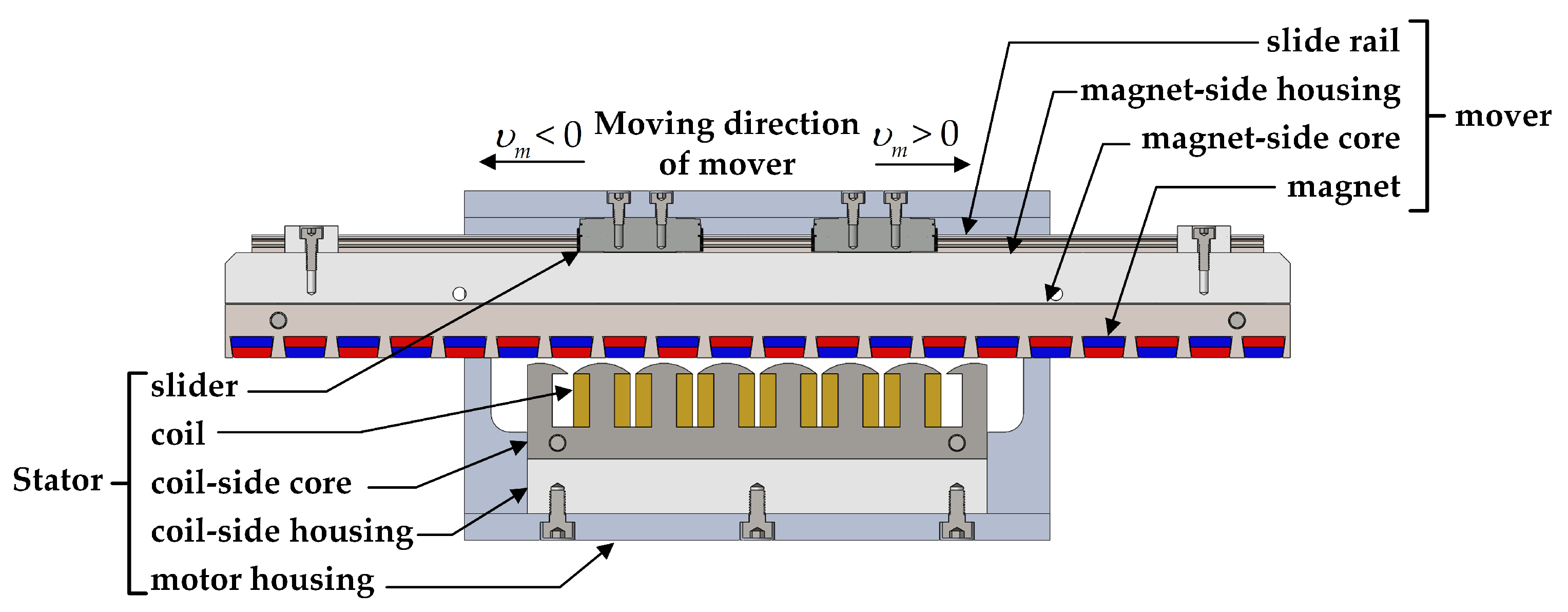
2.1. Structure of Permanent-Magnet Linear Motor
2.2. Auxiliary Core to Improve End Effects
2.3. Electromagnetic Force Analysis and Improvement
3. Control Strategy and Simulation of the Small-Type Permanent-Magnet Linear Motor
3.1. Electromagnetic Force Control Strategy After Cogging Force Improvement
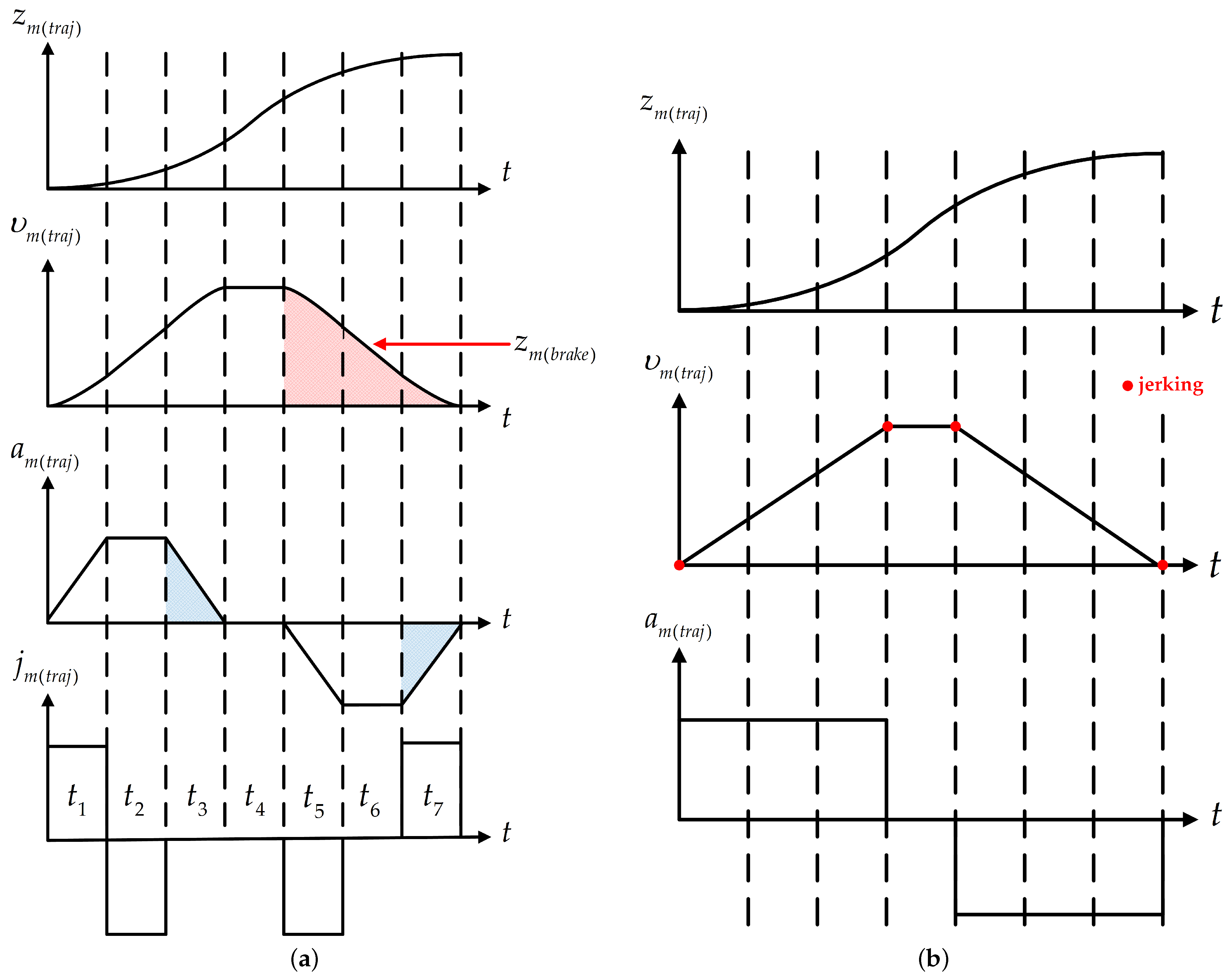
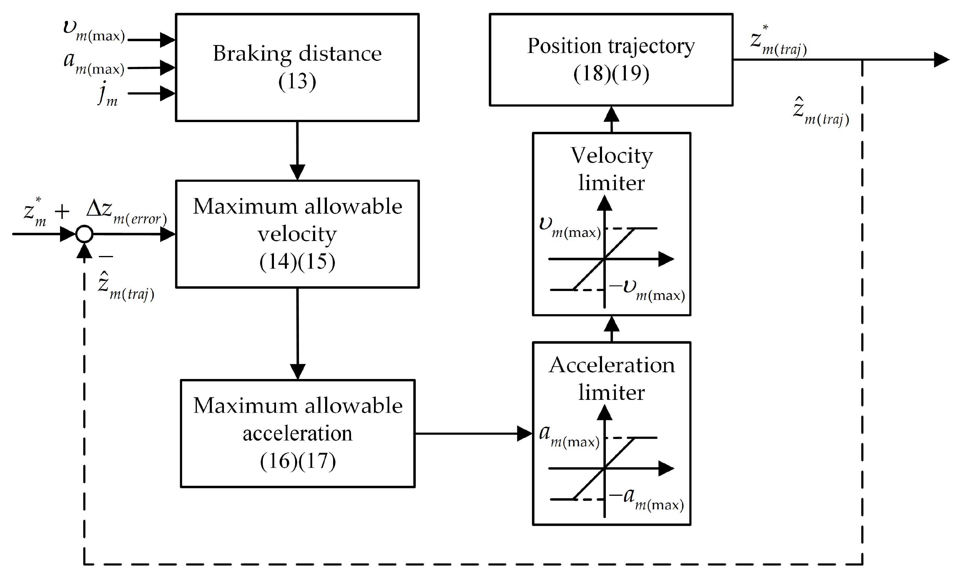
3.2. S-Curve Motion Trajectory Control Strategy
3.3. Control Strategy Simulation
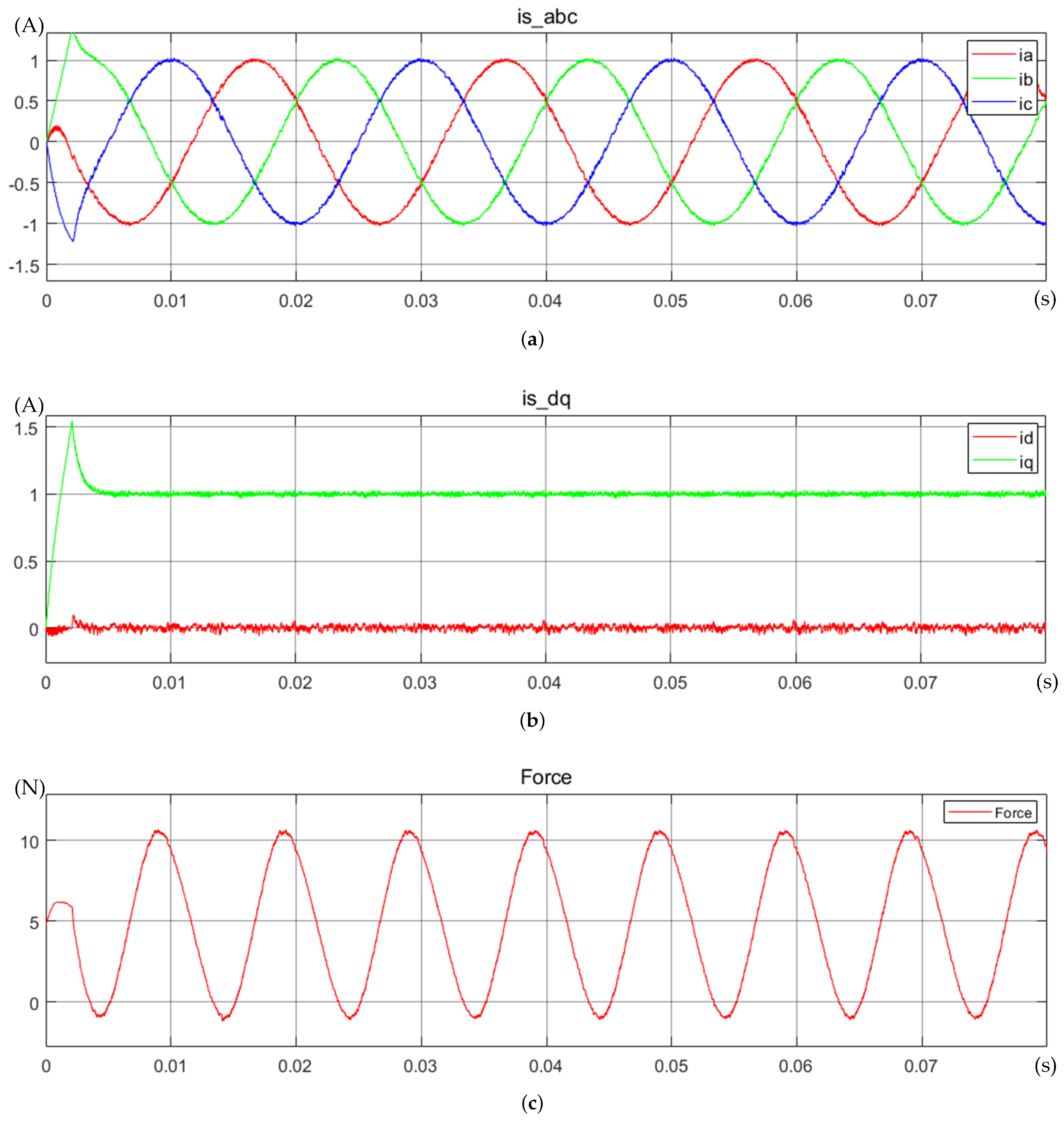
3.3.1. Electromagnetic Force Control Simulation
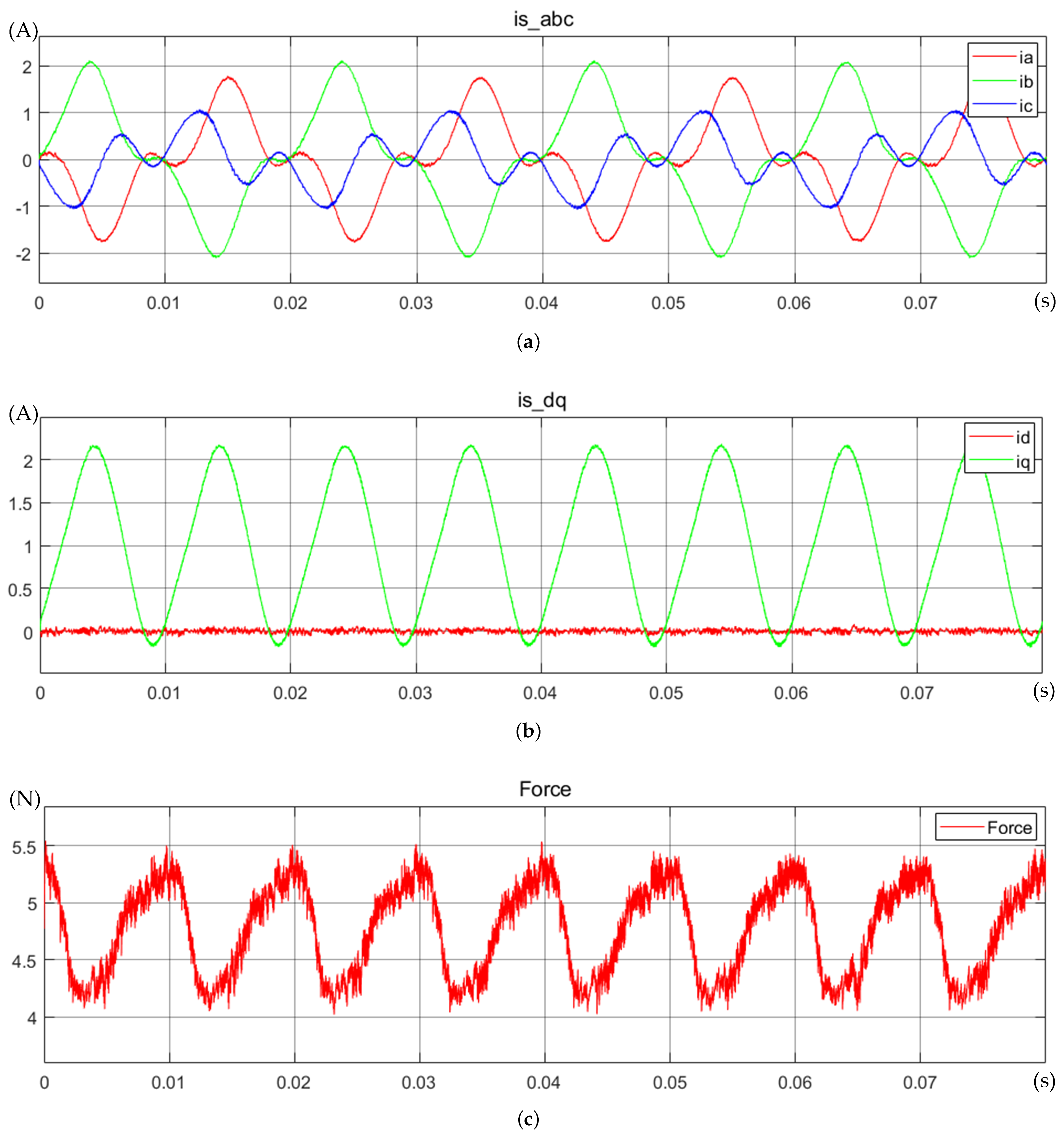
3.3.2. Cogging Force Improvement Simulation
3.3.3. S-Curve Motion Trajectory Control Simulation
4. System Testing
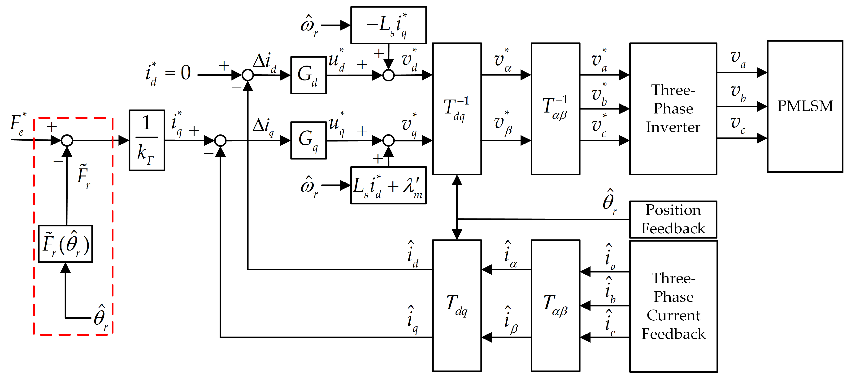
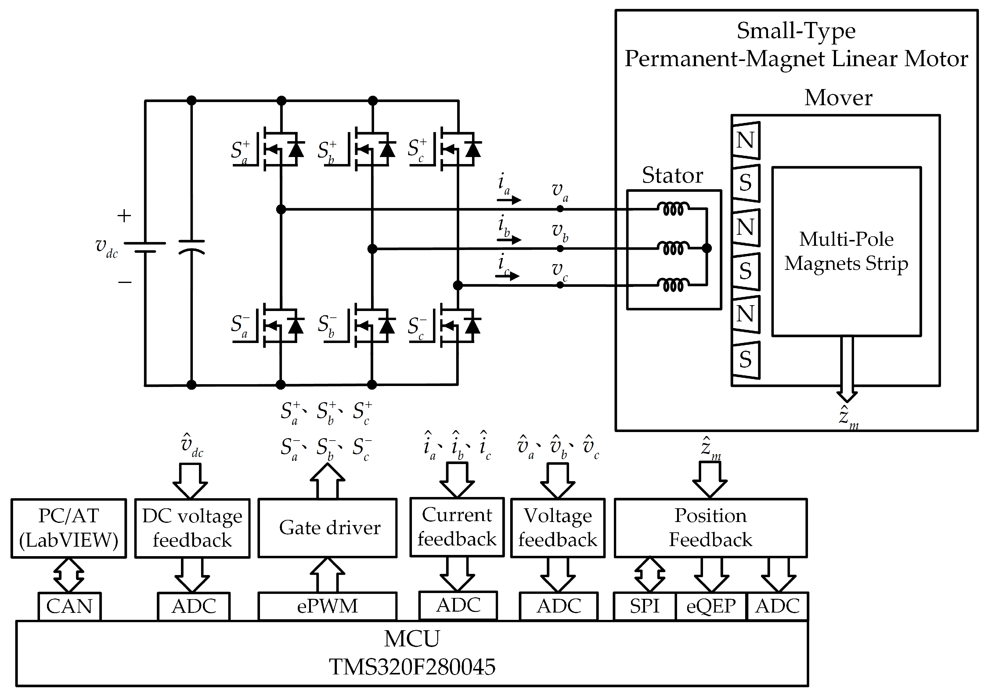
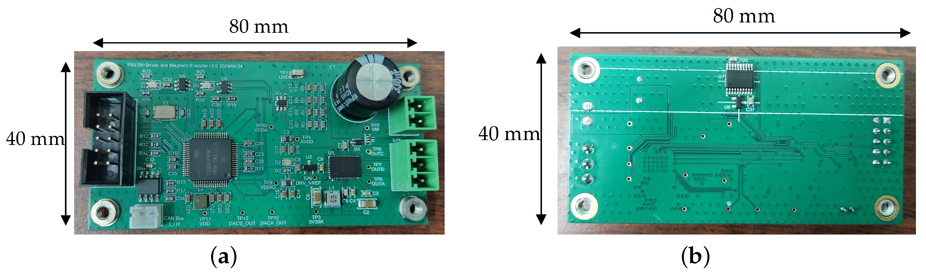
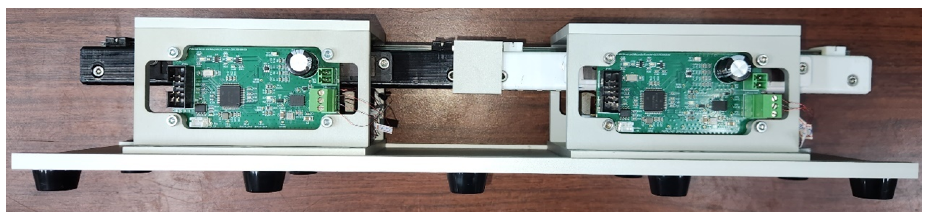
4.1. Drive System Structure
4.2. End Effect Improvement Testing
4.3. Cogging Force Improvement Testing
4.4. S-Curve Motion Trajectory Control Testing
4.5. Simulation and Testing Comparison
5. Conclusions
Author Contributions
Funding
Institutional Review Board Statement
Informed Consent Statement
Data Availability Statement
Conflicts of Interest
References
- Chung, S.U.; Kim, J.M. Double-Sided Iron-Core PMLSM Mover Teeth Arrangement Design for Reduction of Detent Force and Speed Ripple. IEEE Trans. Ind. Electron. 2016, 63, 3000–3008. [Google Scholar] [CrossRef]
- Zhang, Z.; Shi, L.; Wang, K.; Li, Y. Characteristics Investigation of Single-sided Ironless PMLSM Based on Halbach Array for Medium-Speed Maglev Train. CES Trans. Electr. Mach. Syst. 2017, 1, 375–382. [Google Scholar] [CrossRef]
- Hwang, C.C.; Li, P.L.; Liu, C.T. Optimal Design of a Permanent Magnet Linear Synchronous Motor with Low Cogging Force. IEEE Trans. Magn. 2012, 48, 1039–1042. [Google Scholar] [CrossRef]
- Zhu, Y.W.; Cho, Y.H. Thrust Ripples Suppression of Permanent Magnet Linear Synchronous Motor. IEEE Trans. Magn. 2007, 43, 2537–2539. [Google Scholar] [CrossRef]
- Zhu, Y.W.; Jin, S.M.; Chung, K.S.; Cho, Y.H. Control-Based Reduction of Detent Force for Permanent Magnet Linear Synchronous Motor. IEEE Trans. Magn. 2009, 45, 2827–2830. [Google Scholar] [CrossRef]
- Lu, Q.; Wu, B.; Yao, Y.; Shen, Y.; Jiang, Q. Analytical Model of Permanent Magnet Linear Synchronous Machines Considering End Effect and Slotting Effect. IEEE Trans. Energy Convers. 2020, 35, 139–148. [Google Scholar] [CrossRef]
- Hu, H.; Zhao, J.; Liu, X.; Guo, Y. Magnetic Field and Force Calculation in Linear Permanent-Magnet Synchronous Machines Accounting for Longitudinal End Effect. IEEE Trans. Ind. Electron. 2016, 63, 7632–7643. [Google Scholar] [CrossRef]
- Zhang, C.; Zhang, L.; Huang, X.; Yang, J.; Shen, L. Research on the Method of Suppressing the End Detent Force of Permanent Magnet Linear Synchronous Motor Based on Stepped Double Auxiliary Pole. IEEE Access 2020, 8, 112539–112552. [Google Scholar] [CrossRef]
- Shin, K.H.; Kim, K.H.; Hong, K.; Choi, J.Y. Detent Force Minimization of Permanent Magnet Linear Synchronous Machines Using Subdomain Analytical Method Considering Auxiliary Teeth Configuration. IEEE Trans. Magn. 2017, 53, 8104504. [Google Scholar] [CrossRef]
- Kim, S.J.; Park, E.J.; Jung, S.Y.; Kim, Y.J. Optimal Design of Reformed Auxiliary Teeth for Reducing End Detent Force of Stationary Discontinuous Armature PMLSM. IEEE Trans. Appl. Supercond. 2016, 26, 5203305. [Google Scholar] [CrossRef]
- Zhang, H.; Kou, B.; Jin, Y.; Zhang, H. Investigation of Auxiliary Poles Optimal Design on Reduction of End Effect Detent Force for PMLSM With Typical Slot–Pole Combinations. IEEE Trans. Magn. 2015, 51, 8203904. [Google Scholar]
- Cui, L.; Zhang, H.; Jiang, D. Research on High Efficiency V/f Control of Segment Winding Permanent Magnet Linear Synchronous Motor. IEEE Access 2019, 7, 138904–138914. [Google Scholar] [CrossRef]
- Zhao, Z.; Hu, C.; Wang, Z.; Wu, S.; Liu, Z.; Zhu, Y. Back EMF-Based Dynamic Position Estimation in the Whole Speed Range for Precision Sensorless Control of PMLSM. IEEE Trans. Ind. Informatics 2023, 19, 6525–6536. [Google Scholar] [CrossRef]
- Wen, T.; Wang, Z.; Xiang, B.; Han, B.; Li, H. Sensorless Control of Segmented PMLSM for Long-Distance Auto-Transportation System Based on Parameter Calibration. IEEE Access 2020, 8, 102467–102476. [Google Scholar] [CrossRef]
- Sun, X.; Wu, M.; Yin, C.; Wang, S.; Tian, X. Multiple-Iteration Search Sensorless Control for Linear Motor in Vehicle Regenerative Suspension. IEEE Trans. Transp. Electrif. 2021, 7, 1628–1637. [Google Scholar] [CrossRef]
- Xu, W.; Liao, K.; Ge, J.; Qu, G.; Cheng, S.; Wang, A.; Boldea, I. Improved Position Sensorless Control for PMLSM via an Active Disturbance Rejection Controller and an Adaptive Full-Order Observer. IEEE Trans. Ind. Appl. 2023, 59, 1742–1753. [Google Scholar] [CrossRef]
- Wang, M.; Li, L.; Pan, D.; Tang, Y.; Guo, Q. High-Bandwidth and Strong Robust Current Regulation for PMLSM Drives Considering Thrust Ripple. IEEE Trans. Power Electron. 2016, 31, 6646–6657. [Google Scholar] [CrossRef]
- Kung, Y.S. Design and Implementation of a High-Performance PMLSM Drives Using DSP Chip. IEEE Trans. Ind. Electron. 2008, 55, 1341–1351. [Google Scholar] [CrossRef]
- Yuan, H.; Zhao, X. Adaptive Jerk Control and Modified Parameter Estimation for PMLSM Servo System with Disturbance Attenuation Ability. IEEE/ASME Trans. Mechatron. 2023, 28, 164–174. [Google Scholar] [CrossRef]
- Rew, K.H.; Kim, K.S. A Closed-Form Solution to Asymmetric Motion Profile Allowing Acceleration Manipulation. IEEE Trans. Ind. Electron. 2010, 57, 2499–2506. [Google Scholar] [CrossRef]
- Bai, Y.; Chen, X.; Sun, H.; Yang, Z. Time-Optimal Freeform S-Curve Profile Under Positioning Error and Robustness Constraints. IEEE/ASME Trans. Mechatron. 2018, 23, 1993–2003. [Google Scholar] [CrossRef]
- Ha, C.W.; Rew, K.H.; Kim, K.S.; Kim, S. Tuning the S-curve Motion Profile in Short Distance Case. In Proceedings of the 2013 American Control Conference, Washington, DC, USA, 17–19 June 2013; pp. 4975–4980. [Google Scholar]
- Ha, C.W.; Rew, K.H.; Kim, K.S. Robust Zero Placement for Motion Control of Lightly Damped Systems. IEEE Trans. Ind. Electron. 2013, 60, 3857–3864. [Google Scholar] [CrossRef]


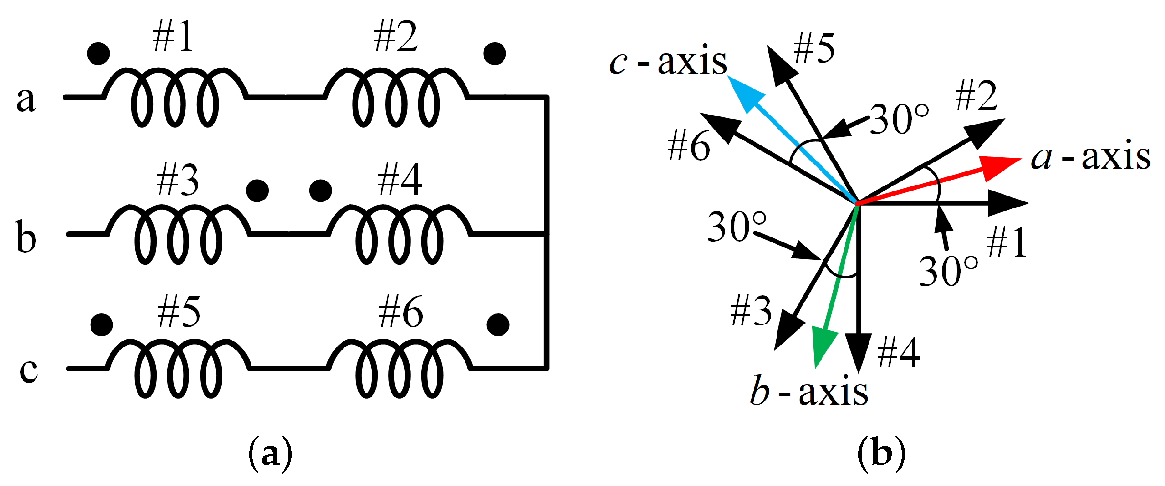
| Number of Coil | #1 | #2 | #3 | #4 | #5 | #6 |
|---|---|---|---|---|---|---|
| Electrical angle | 0° | 210° (30°) | 60° (240°) | 270° | 120° | 330° (150°) |
| Number of phases | a+ | a− | b− | b+ | c+ | c− |
| Mover | trapezoidal magnet | material | sintered NdFeB magnet N35 |
| width of the long side | 8 | ||
| width of the short side | 7 | ||
| height | 4 | ||
| pole pitch | 10 | ||
| core | material | silicon steel sheet 50CS600 | |
| length | 200 | ||
| width | 17 | ||
| height | 10 | ||
| air gap | 1 | ||
| Stator | coil | material | polyurethane enamelled copper wire |
| wire diameter | 0.25 | ||
| length | 23 | ||
| width | 10.67 | ||
| height | 10 | ||
| core | material | silicon steel sheet 50CS600 | |
| length | 86.33 | ||
| width | 17 | ||
| height | 18 | ||
| front iron height | 2 | ||
| back iron height | 6 | ||
| Auxiliary Core | Without | With | |
|---|---|---|---|
| Phase a back-EMF | fundamental (V) | 3.735 | 3.619 |
| THD (%) | 3.93 | 0.58 | |
| Phase b back-EMF | fundamental (V) | 3.929 | 3.621 |
| THD (%) | 0.68 | 0.40 | |
| Peak back-EMF difference between phase a and b (V) | −0.194 | −0.002 | |
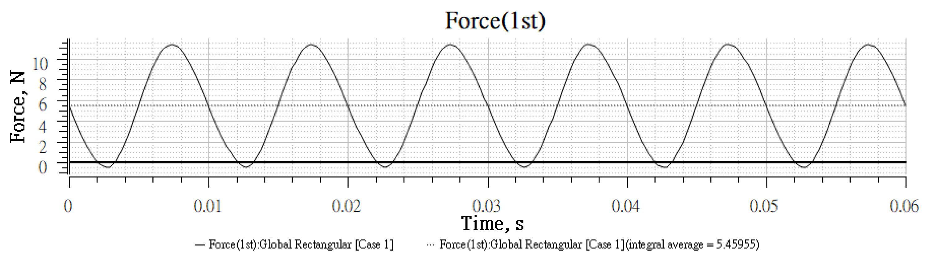
| Harmonic Order | Harmonic Amplitude (N) | Phase Angle (°) |
|---|---|---|
| 2 | 6.05 | 119.7 |
| 4 | 0.42 | 238.4 |
| 6 | 0.21 | 198.7 |
| 8 | 0.08 | −53.6 |
| Improvement Items | Comparison Items | Simulation | Testing |
|---|---|---|---|
| End effect improvement | (V/(rad/s)) | 0.0115 | 0.0104 |
| a phase voltage balance error (V) | 0.002 | 0.020 | |
| Cogging force improvement | q-axis current compensation (A) | ±1.12 | ±1.05 |
| result | ±0.5 N electromagnetic force ripple | Able to move smoothly with any load | |
| S-curve motion trajectory control | steady-state speed error (m/s) | 0.02 | 0.03 |
| steady-state position error (μm) | 60 | 5 |
Disclaimer/Publisher’s Note: The statements, opinions and data contained in all publications are solely those of the individual author(s) and contributor(s) and not of MDPI and/or the editor(s). MDPI and/or the editor(s) disclaim responsibility for any injury to people or property resulting from any ideas, methods, instructions or products referred to in the content. |
© 2024 by the authors. Licensee MDPI, Basel, Switzerland. This article is an open access article distributed under the terms and conditions of the Creative Commons Attribution (CC BY) license (https://creativecommons.org/licenses/by/4.0/).
Share and Cite
Ho, C.-H.; Hwang, J.-C. Design of Small Permanent-Magnet Linear Motors and Drivers for Automation Applications with S-Curve Motion Trajectory Control and Solutions for End Effects and Cogging Force. Energies 2024, 17, 5719. https://doi.org/10.3390/en17225719
Ho C-H, Hwang J-C. Design of Small Permanent-Magnet Linear Motors and Drivers for Automation Applications with S-Curve Motion Trajectory Control and Solutions for End Effects and Cogging Force. Energies. 2024; 17(22):5719. https://doi.org/10.3390/en17225719
Chicago/Turabian StyleHo, Chia-Hsiang, and Jonq-Chin Hwang. 2024. "Design of Small Permanent-Magnet Linear Motors and Drivers for Automation Applications with S-Curve Motion Trajectory Control and Solutions for End Effects and Cogging Force" Energies 17, no. 22: 5719. https://doi.org/10.3390/en17225719
APA StyleHo, C.-H., & Hwang, J.-C. (2024). Design of Small Permanent-Magnet Linear Motors and Drivers for Automation Applications with S-Curve Motion Trajectory Control and Solutions for End Effects and Cogging Force. Energies, 17(22), 5719. https://doi.org/10.3390/en17225719