Dynamic Environmental Economic Dispatch Considering the Uncertainty and Correlation of Photovoltaic–Wind Joint Power

Abstract

The traditional power grid planning lacks consideration of the uncertainty and correlation between wind and solar joint output in the same region, which poses challenges to the stable operation of the power system. Therefore, it is greatly important to consider the environmental and economic dispatch in light of the uncertainties and correlations associated with wind and solar energy. To tackle these issues, this paper introduces a dynamic environmental economic dispatch model that accounts for the uncertainties and correlations between wind and photovoltaic power based on their output characteristics. Initially, a probability model for photovoltaic–wind joint power is established using the Copula function. Subsequently, the Latin hypercube sampling method is employed alongside an improved K-means clustering technique to derive typical output scenarios. An adaptive multi-objective fireworks algorithm, featuring a differential selection strategy, is then utilized to enhance the environmental economic dispatch model. Finally, the IEEE 39 node system is used as an example to demonstrate the solution of the dynamic environmental and economic scheduling model. Simulation results reveal that the method for generating typical output scenarios presented in this paper effectively captures the uncertainties and correlations of photovoltaic–wind joint power. Furthermore, when compared to other optimization algorithms, the improved adaptive multi-objective fireworks algorithm proves to be more efficient in addressing the dynamic environmental economic dispatch challenges within the power system.

1. Introduction

Environmental economic dispatch (EED) refers to the power system dispatch that optimizes both fuel costs and pollution emissions as objectives, and it has gradually become one of the important ways for emissions reduction in the power industry [1]. The power industry has been increasing the development and utilization of renewable and clean energy sources, and the rapid development of new energy sources represented by wind and photovoltaic has brought about environmental and economic benefits that cannot be ignored. However, the new energy output of wind power and photovoltaic power has strong uncertainty. The wind farms and photovoltaic power plants in the same area have a certain correlation in output [2]. The traditional output model cannot accurately describe its output characteristics, which brings new problems and challenges to the power grid planning [3,4]. Therefore, it is of great significance to study the environmental economic dispatch considering the uncertainty and correlation of photovoltaic–wind joint power [5].

In the study of the characteristics of wind power and photovoltaic power, the key lies in accurately establishing mathematical models for wind and photovoltaic power outputs and using these models to investigate their impact on the system. At present, the research on photovoltaic–wind joint power characteristics is mainly focused on uncertainty and correlation. For the uncertainty of photovoltaic–wind joint power, investigating the literature [6] based on generative adversarial network combined with conditional risk for scenario generation is necessary to obtain the wind power time series model. Reference [7] chooses the Monte Carlo method to extract random components to obtain PV output time series. The time series model can better reflect the specific power output situation of the wind and photovoltaic, but there are big limitations in describing the changes in power output under different weather conditions. For the photovoltaic–wind joint power correlation, reference [8] through the nonparametric kernel density estimation method of the annual wind speed showed that light intensity data are fitted to obtain the photovoltaic–wind joint power distribution model, and the Copula function is selected as the joint probability distribution model of wind distribution. Reference [9] selected the Copula function combined with the Gaussian model fitting to obtain its distribution model. Reference [10] used the kernel density estimation method to find out the marginal probability distribution function, and then based on the dynamic C cane pair-Copula theory to obtain the joint distribution function of wind–photovoltaic power joint treatment. The above studies have explored the characteristics of wind and photovoltaic power. However, there is a lack of research that comprehensively considers the uncertainty and correlation of photovoltaic–wind joint power in the same region, and there is a lack of application in the planning of power grids.

The Dynamic Environmental Economic Dispatch (DEED) of the power system is a scheduling model to minimize the unit output cost and unit pollution emission during the scheduling cycle [11,12]. Compared with Dynamic Economic Dispatch (DED) and Dynamic Environmental Dispatch (EED), DEED has the characteristics of high dimensionality, strong constraints, nonlinearity, and nonconvexity [13,14]. Meanwhile, it has two optimization objective functions and there is a coupling relationship between the functions, which makes the model solution more complicated after considering the uncertainty and correlation of the combined output of wind and light. Reference [15] utilizes a chaotic encryption algorithm to transform the local optimal value obtained by PSO optimization into global optimal value. Reference [16] considers constraints such as wind turbine output, thermal power output, and climbing, and utilizes the neural network-based nonlinear model built using exogenous variables (NLARX) to obtain the optimal solution for the system. Reference [17] uses particle swarm algorithm to determine the scheduling strategy for minimum power generation cost for the system. Reference [18] adopts a fuzzy optimization strategy to solve the scheduling problem of the model. Reference [19] is based on the Improved Reactor Optimization Algorithm (RDHBO) to solve the dynamic economic dispatch of electric vehicles connected to the grid, which improves the accuracy and convergence speed of the algorithm. Reference [20] proposes a local search DE algorithm based on elite cloning. To improve the algorithm’s mining and exploration capabilities, a cloning and mutation mechanism for elite groups is added, effectively enhancing the algorithm’s global search ability. Reference [21] proposes an adaptive multi-objective differential evolution algorithm, which effectively improves the exploration and mining capabilities of traditional evolutionary algorithms by designing an adaptive current to best/1 crossover operator. However, the above algorithms for multi-objective problems, towards a certain local objective optimization, cannot obtain a uniformly distributed Pareto optimal frontier; heuristic algorithms that can efficiently find the optimal algorithms and fast and effective constraints processing strategy become the key to solving the DEED problem.

Aiming at the DEED problem and the current deficiencies of heuristic algorithms, this paper proposes a dynamic environmental economic dispatch model based on a multi-objective fireworks algorithm by considering the uncertainty and correlation of photovoltaic–wind joint power and generation scene aggregation of photovoltaic–wind joint power. Firstly, for the output characteristics of wind power and photovoltaic power, the non-parametric kernel density estimation method is used to establish a joint output model with photovoltaic–wind joint power uncertainty and correlation; secondly, the joint output probability model of photovoltaic–wind joint power is established by the Copula function, and at the same time, the joint output scenarios of wind and photovoltaic are generated based on the Latin Hypercubic Sampling Method and the Improved K-means Clustering Algorithm; and lastly, an Improved Fireworks Combined with Difference Selection Policy algorithm (ADMOFWA) is proposed to solve the dynamic economic dispatch model considering wind-scenery access to the grid.

The main contributions of this paper are as follows.

(1)

It proposes a novel dynamic environmental economic dispatch model based on a multi-objective fireworks algorithm, specifically tailored to tackle the DEED problem and address the limitations observed in existing heuristic algorithms.

(2)

The utilization of the non-parametric kernel density estimation method to construct a joint output model for both wind and photovoltaic power sources represents a pioneering approach in capturing and integrating uncertainty and correlation factors.

(3)

Through the application of the Copula function, the research establishes a robust joint output probability model for photovoltaic–wind joint power, facilitating the generation of realistic joint output scenarios via the innovative combination of the Latin Hypercubic Sampling Method and the Improved K-means Clustering Algorithm.

(4)

The improved fireworks algorithm (IFWA) is proposed for the optimal solution of the power system planning problem. This algorithm improves the way fireworks are initially generated based on the basic fireworks algorithm. It also optimizes the explosion and mutation operators by combining adaptive operators and the idea of differential evolution algorithm and introduces a selection strategy based on fitness values for elite preservation. At the same time, the random selection method for the roulette wheel in the basic fireworks algorithm is replaced with binary search to effectively improve computational efficiency.

2. Generation and Reduction in Scenery Scenes

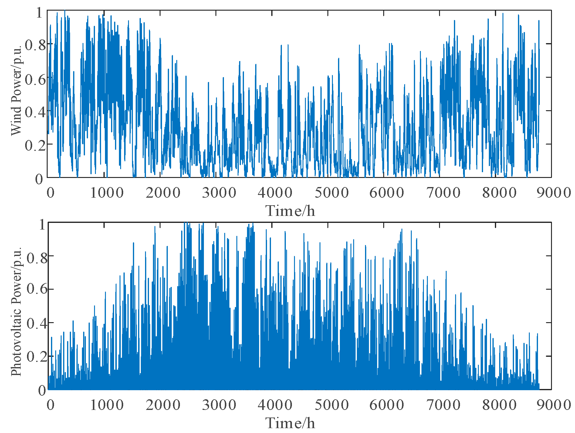
2.1. Output Model for Wind Power Generator

The wind turbine has great uncertainty in output. According to many theoretical studies, the random behavior of wind speed has certain distribution characteristics which are called skewed distribution. In mathematics, the two-parameter Weibull distribution can be used to accurately fit the measured wind speed data. From [22], the probability density distribution function of wind speed can be described as:

$$f_w(v_t)={\displaystyle \frac{k}{c}}{\left({\displaystyle \frac{v_t}{c}}\right)}^{k-1}{e}^{\left[-{\left({\displaystyle \frac{v_t}{c}}\right)}^k\right]},$$

(1)

where $v_t$ denotes the predicted average wind speed of the wind field, k and c denote the probability distribution shape parameter and scale parameter, respectively.

The output power for a given wind speed is:

$$P_w=\left\{\begin{array}{c}0, 0\le v_t\le v_{ci} , v_t>v_{co}\\ {\displaystyle \frac{P_r}{v_r-v_{ci}}}-{\displaystyle \frac{P_r{v}_{ci}}{v_r-v_{ci}}}, v_{ci}<v_t\le v_r\\ P_r, v_r<v_t\le v_{co}\end{array}\right.,$$

(2)

where $v_t$ denotes the wind speed, $v_{ci}$ denotes the cut-in wind speed, $v_{co}$ denotes the cut-out wind speed, $v_r$ denotes the rated wind speed of the wind turbine, and $P_r$ denotes the rated output power of the wind turbine.

2.2. Output Model for Photovoltaic Generator

The photovoltaic output is usually simulated using a beta distribution, and its probability density function is expressed as [23]:

$$f_s(E_t)={\displaystyle \frac{\mathsf{\Gamma }(\alpha +\beta )}{\mathsf{\Gamma }(\alpha )\mathsf{\Gamma }(\beta )}}{\left({\displaystyle \frac{E_t}{E_{\max }}}\right)}^{\alpha -1}{\left(1-{\displaystyle \frac{E_t}{E_{\max }}}\right)}^{\beta -1},$$

(3)

where $E_t$ denotes the actual light intensity, $E_{\max }$ denotes the maximum light intensity, $\mathsf{\Gamma }$ denotes the gamma function, $\alpha$ and $\beta$ denote both shape parameters.

For a given light Radiant intensity, the photovoltaic output can be expressed as:

$$P_{pv}=E_t\cdot S\cdot \tau ,$$

(4)

where S denotes the area of the photovoltaic panel and $\tau$ denotes the conversion efficiency between light energy and electrical energy.

2.3. Scenario Generation and Reduction

Combined with the above probability distribution model of wind and photovoltaic power, the Latin hypercube sampling method is used for random sampling, and the probability distribution model is dispersed using the sampling method to obtain $n$ wind power and photovoltaic output scene datasets. The Latin hypercube sampling method is a quasi-random sampling technique that is used to generate parameter values from a multidimensional distribution. It is known for its ability to reduce the number of iterations required for sampling while maintaining high sampling accuracy with a smaller sample size compared to the commonly used Monte Carlo method [24].

After obtaining a large number of wind and photovoltaic output scenarios, the data scale becomes large, and it can also increase the complexity of subsequent model-solving algorithms. Therefore, scene reduction is required for many scenarios [25]. The specific steps for scene reduction can be concluded as follows:

(1) Obtain the generated dataset of $n$ wind, and photovoltaic output scenes $S=\{s_1,s_1,\dots ,s_n\}$ and the probability of scene occurrence;

(2) Calculate the Euclidean distance $d$ between the $i-th$ and $j-th$ scenes in the scene set:

$$d(s_i,s_j)=\sqrt{{\displaystyle \sum _{w=1}^z\left(s_{iw}-s_{jw}\right)}},$$

(5)

where $s_i$ and $s_j$ denote the ith and jth scenes in the scenery scene set, $z$ is the number of sample sampling instant. Each scene, and the obtained Euclidean distance is stored in the distance distribution matrix $D$;

(3) Obtain the initial clustering center based on the principle of maximum and minimum distance, allocate all scenes to various clusters according to the minimum distance, and update the probability of each cluster scene set according to:

$$p_{C_i}=N_i/n,$$

(6)

where $p_{C_i}$ denotes the probability of the set $C_i$ typical scenario in ith scenario class cluster. $N_i$ denotes the number of scenes in the collection $C_i$, and $n$ denotes the total number of scenes in the initial wind and photovoltaic output scene S;

(4) Repeat the steps until the scene is reduced to the specified desired number.

3. DEED Model

3.1. Objective Functions

The model optimizes and solves the thermal cost of electricity by using source $F_1$ and pollution emission cost $F_2$ in each dispatching period $t$ [26].

Objective functions:

(1) In a thermal power plant, the active output of the generator is controlled by adjusting the opening and closing of multiple steam valves. The gradual opening or closing of these valves, along with the phenomenon of wire drawing, exhibits nonlinearity, which can lead to spontaneous or sudden increases in losses. This results in a highly nonlinear power output from the generator, producing a pulsating effect similar to the coal consumption characteristics, known as the valve point effect. When calculating the fuel costs for the unit, it is essential to consider the nonlinear power variations caused by the valve point effect. Therefore, a sine function has been incorporated into the secondary cost function to represent the ripple effect generated by the opening of the steam valves, ultimately minimizing the costs of the thermal power unit:

$$F_1\left(P\right)={\displaystyle \sum _{s=1}^{Ns}{\rho }_s\left({\displaystyle \sum _{t=1}^T{\displaystyle \sum _{i=1}^N\left\{a_i+b_i{P}_{s,i,t}+c_i{P}_{s,i,t}^2+\right.}}\right.} \left.\left|d_i\sin \left[e_i\left(P_t^{\min }-P_{\mathrm{s},\mathrm{i},\mathrm{t}}\right)\right]\right|\right\}),$$

(7)

where ${\rho }_s$ denotes the probability of scenario s, $N_s$ denotes the total number of scenarios, T is the total scheduling period, N denotes the total number of thermal power units, $a_i$, $b_i$, $c_i$, $d_i$, $e_i$ denote the cost coefficients of the ith thermal power unit, respectively, and $P_{\mathrm{s},\mathrm{i},\mathrm{t}}$ denotes the power generation output of thermal power unit $i$ in period t under scenario s.

(2) Minimal cost of pollution can be established as:

$$F_2\left(P\right)={\displaystyle \sum _{s=1}^{Ns}{\rho }_s\left({\displaystyle \sum _{t=1}^T{\displaystyle \sum _{i=1}^N\left({\alpha }_i+{\beta }_i{P}_{s,i,t}+{\gamma }_i{P}_{s,i,t}^2\right)}}+\right.}{\xi }_i\exp \left({\lambda }_i{P}_{s,i,t}\right)),$$

(8)

where ${\alpha }_i$, ${\beta }_i$, ${\gamma }_i$, ${\xi }_i$, ${\lambda }_i$ denote the pollution emission coefficients of each thermal power unit.

3.2. Constraint Function

3.2.1. System Power Balance Constraints

Within unit time t, the system power must meet the equation constraints as follows:

$${\displaystyle \sum _{i=1}^N{P}_{i,t}}+P_t^{\mathrm{w}}+P_t^{\mathrm{pv}}=L_t+P_t^{\mathrm{loss}},$$

(9)

where $P_{i,t}$ denotes the output power of the ith thermal power unit in unit time t, $P_t^W$ and $P_t^{PV}$ denote the outputs of wind power and photovoltaic power in period t, $L_t$ denotes the load at time t. The network loss $p_t^{loss}$ can be calculated by using

$$P_t^{\mathrm{loss} }={\displaystyle \sum _i^N{\displaystyle \sum _j^N{P}_i}}{B}_{i,j}{P}_j+{\displaystyle \sum _i^N{P}_i}{B}_{i,0}+B_{0,0},$$

(10)

where $B_{i,j}$, $B_{i,0}$, $B_{0,0}$ denote network loss coefficients.

3.2.2. Power Generation Capacity Constraints

The constraints to be met by thermal power generating units are as follows:

$$P_i^{\min }<P_{i,t}<P_i^{\max },$$

(11)

where $P_i^{\max }$ and $P_i^{\min }$ denote the upper and lower limits of the output of the thermal motor group $i$.

3.2.3. Ramp Rate Constraints for Thermal Power Units

The ramp rate constraints that thermal power units need to satisfy are as follows:

$$\left\{\begin{array}{l}{P}_{i,t}-P_{i,t-1}<U{R}_i\cdot \Delta t\hfill \\ P_{i,t-1}-P_{i,t}<D{R}_i\cdot \Delta t\hfill \end{array}\right.,$$

(12)

where $U{R}_i$ and $D{R}_i$ denote the climbing rate of the ascending and descending of the thermal generating $i$.

3.2.4. System Spare Capacity Constraints

For the stable operation of the power system, it is usually necessary to consider a certain amount of standby capacity to cope with possible unit failures and load forecast errors. The positive and negative rotating standby capacity constraints for the system without new energy access are as follows:

positive rotating standby constraint for the system without new energy access:

$$\left\{\begin{array}{l}{k}^{\mathrm{l}}{L}_t^{\mathrm{f}}\le r_t^{\mathrm{u}}={\displaystyle \sum _{n=1}^N{r}_{n,t}^{\mathrm{u}}}\hfill \\ r_{n,t}^{\mathrm{u}}=\min \left(P_n^{\max }-P_{n,t},U{R}_n\cdot \Delta t\right)\hfill \end{array}\right.,$$

(13)

negative rotating standby constraint for the system without new energy access:

$$\left\{\begin{array}{l}{k}^{\mathrm{l}}{L}_t^{\mathrm{f}}\le r_t^{\mathrm{d}}={\displaystyle \sum _{n=1}^N{r}_{n,t}^{\mathrm{d}}}\hfill \\ r_{n,t}^{\mathrm{d}}=\min \left(P_{n,t}-P_n^{\min },D{R}_n\cdot \Delta t\right)\hfill \end{array}\right.,$$

(14)

where $k^{\mathrm{l}}$ denotes the demand coefficient of the system load forecast error on the positive rotating standby, and $r_t^{\mathrm{u}}$ and $r_t^{\mathrm{d}}$ denote the total positive and negative rotating standby capacity that the system can carry at time t, respectively.

In sources such as wind power, photovoltaic, and other new energy access systems, there is a prediction error due to the uncertainty of wind power. When its power fluctuates, the need for greater system rotating standby capacity to balance the risk of comprehensive consideration of the proposed access to the new energy power system after the positive and negative rotating standby capacity is as follows:

consider the positive rotating standby constraint of the new energy access system:

$$\left\{\begin{array}{l}{k}^{\mathrm{l}}{L}_t^{\mathrm{f}}+k^{\mathrm{e}}{E}_t^{\mathrm{f}}\le r_t^{\mathrm{u}}={\displaystyle \sum _{n=1}^N{r}_{n,t}^{\mathrm{u}}}\hfill \\ r_{n,t}^{\mathrm{u}}=\min \left(P_n^{\max }-P_{n,t},U{R}_n\cdot \Delta t\right)\hfill \end{array}\right.,$$

(15)

consider the negative rotating standby constraint of the new energy connection system:

$$\left\{\begin{array}{l}{k}^{\mathrm{l}}{L}_t^{\mathrm{f}}+k^{\mathrm{e}}{E}_t^{\mathrm{f}}\le r_t^{\mathrm{d}}={\displaystyle \sum _{n=1}^N{r}_{n,t}^{\mathrm{d}}}\hfill \\ r_{n,t}^{\mathrm{d}}=\min \left(P_{n,t}-P_n^{\min },U{R}_n\cdot \Delta t\right)\hfill \end{array}\right.,$$

(16)

where $k^{\mathrm{e}}$ denotes the demand coefficient of the system rotating reserve required by the new energy prediction error, and $E_t^{\mathrm{f}}$ denotes the sum of the new energy output of the system at time t.

4. Adaptive Multi-Objective Fireworks Algorithm

4.1. Algorithm Initialization

For the basic fireworks algorithm, when the initial explosion generates an initial population, due to the randomness of the initial explosion, it may lead to local search wasting some computational resources during the initial iteration process. Therefore, we should firstly improve the initialization of the generated population by dividing the initial explosion population into N equal parts, and randomly exploding the space after each equal part to generate a set of initial fireworks, to ensure global search in the early stages of the algorithm [27].

Figure 1 shows the initial distribution of fireworks generated by the original fireworks algorithm.

When fireworks explode, the better fitness of the fireworks can generate the more sparks, which means that the explosion intensity is greater. The calculation formula for the explosion intensity of each firework can be shown as:

$$S_i=m{\displaystyle \frac{Y_{\max }-f\left(x_i\right)+\theta }{{\displaystyle \sum _{i=1}^{pop}\left(Y_{\max }-f\left(x_i\right)\right)}+\theta }},$$

(17)

where $S_i$ denotes the number of sparks generated by the ith fireworks, $m$ is a constant representing the number of sparks that generated the most, $Y_{\max }$ denotes the worst fitness fireworks in the population, and $f(x_i)$ denotes the fitness function value of the ith fireworks, $\theta$ denotes a sufficient small number of machines to prevent zero division operations, and $pop$ denotes the total number of fireworks populations.

During the explosion process of fireworks, the original fireworks algorithm calculates the explosion radius of fireworks by basing on their fitness. However, due to the presence of multiple fireworks with the same fitness values, different positions in multidimensional can cause optimization problems. Therefore, the fitness optimal spark set sparkpBest and the population optimal firework individual gBest are obtained by introducing each firework explosion. The new explosion radius formula can be represented as [28]:

$$A(i)=\left\{\begin{array}{ll} sparkpBest (i)-x(i),\hfill & S_i<AvgS\hfill \\ gBest-x(i),\hfill & S_i⩾AvgS\hfill \end{array}\right.,$$

(18)

where $sparkpBest (i)$ denotes the optimal individual in the population of sparks generated by the ith fireworks explosion, and AvgS denotes the average of all explosion sparks.

On this basis, a Gaussian mutation is randomly selected for the globally optimal individual gBest to enhance the algorithm’s global search ability, which is a Gaussian distribution function with a mean of 0 and a variance of 1.

The basic fireworks algorithm flowchart is as follows (Figure 2):

4.2. Evolutionary Strategy

For multi-objective evolutionary optimization problems, each objective usually has a mutual constraint relationship. The Pareto method excludes many non-dominated individuals through classification, thereby obtaining a solution set with better convergence. Meanwhile, applying the distribution preserving mechanism to the algorithm can maintain its distribution performance without affecting its convergence. Therefore, each objective solution is measured by Pareto superiority, and different objectives are divided into different levels. That is, for everyone in the population P and non-dominated file NP, its dominance strength value can be calculated by according to the Formula (15), and the superiority of different solutions is measured by basing on the dominance strength of

$$s\left(x_i\right)=\left|x_j\in P\cup NP|x_i\to x_j\right|,$$

(19)

After each iteration, k solutions in the fireworks population are selected through roulette wheel gambling, and then differential evolution is performed on the solutions. The specific steps for evolutionary strategy can be concluded as follows:

• For each solution x in the solution set obtained above, the other two solutions are randomly selected, and their differences are weighted and added to the original solution to obtain the mutation solution of the original solution $v_i$;
• Cross mutation solution and several elements in the original solution, resulting in a cross solution $u_i$. The method for selecting the j-th element in the cross solution is shown:

  $$u_i^j=\left\{\begin{array}{l}{v}_i^j,\mathrm{rand}(0,1)<C_r \mathrm{or} j=r(i)\\ x_i^j, \mathrm{else}\end{array}\right.,$$

  (20)

  where $C_r$ denotes a constant between $[0,1]$, $r(i)$ denotes the probability of crossing, A random number is taken within $(0,N]$;
• Choose the cross solution and the better solution from the original solution to join the next generation. If the cross solution is selected, the fitness function is used to determine whether it is a non-dominant solution within the contemporary solution. If so, it is also needed to update NP, which is shown as:

  $$x_i=\left\{\begin{array}{c}{u}_i,f\left(u_i\right)\le f\left(x_i\right)\\ x_i, \mathrm{else} \end{array}\right.,$$

  (21)

4.3. Selecting Strategy Improvements

The selection strategy of the basic fireworks algorithm is based on the roulette wheel rule of Euclidean distance. This approach necessitates the computation of the Euclidean distance between any two individuals in the population, which significantly increases the algorithm’s solution time and memory consumption. Therefore, this section adopts an elite retention strategy based on fitness values to address this issue:

• The elite individuals with the best fitness from the current fireworks, explosion sparks, and mutation sparks populations are directly preserved in the next generation of explosion fireworks. This ensures that the optimal individuals are not lost. For the remaining N-1 fireworks with relatively high fitness that were not selected, it is important to note that the best few sparks may originate from a single firework. This could lead to a situation where a locally optimal firework is not easily eliminated, resulting in a weakened global search capability of the algorithm. Thus, direct selection is not feasible, and it is necessary to continue integrating subsequent selection strategies.
• Calculate the fitness difference between different fireworks and sparks $\Delta f(x)$. Select fireworks with an internal fitness that is superior, where $\Delta f(x)$ is less than $\gamma$ ($\gamma$ being a constant that filters for fireworks with similar fitness values).

  $$\Delta f(x)=f(x_i)-f(x_j),$$

  (22)

  where $f(x_i)$ and $f(x_j)$ represent the fitness of fireworks $x_i$ and $x_j$, respectively.
• After the second round of screening, N−1 fireworks are randomly selected to proceed to the next generation, ensuring population diversity.
  In addition, regarding the roulette wheel selection method of the basic fireworks algorithm, it is necessary to traverse the entire population to calculate and set the weight of each firework individual. Based on the Euclidean distance calculation method, its time complexity is $O(n^2)$. This paper improves upon this by employing a binary search method; for each query, a random number is generated for the firework individual, and then binary search is utilized for the query, resulting in a time complexity of $O(\log n)$. This approach can significantly enhance computational efficiency, especially when dealing with larger populations.

The algorithm for improving the fireworks is as shown in the following diagram (Figure 3):

Figure 3. The algorithm for improving the fireworks flowchart.

Figure 3. The algorithm for improving the fireworks flowchart.

The algorithm implementation Pseudocode is as follows (Algorithm 1):

Algorithm 1: ADMOFWA Pseudocode

1. Start;

2. Divide the entire solution space N equally, and randomly explode a set of initial fireworks in each population;

3. Record the global optimal gBest, the set of sparkpBest for the optimal explosive sparks generated by each firework, obtain the fitness value of each firework, and form the solution set P;

4. Create an empty non dominated solution set NP;

5. When the number of iterations iter < max_itr;

6. For each firework $x_i$ in solution P, calculate the number of explosive sparks for each firework according to the equation;

7. Calculate the explosion radius of each firework according to the formula to generate sparks, and update SparkpBest to generate sparks for Gaussian explosions;

8. Acquire the fitness values for all sparks;

9. Update NP by selecting non-dominated solutions from sparks;

10. Using roulette to choose n solutions from fireworks and sparks;

11. Decompose each firework $x_i$ in the fireworks set P;12. Obtain a crossover solution based on crossover, mutation, and selection $u_i$. If the fitness value of the crossover solution is better than $x_i$, use $u_i$ to update NP;

13. Select an optimal solution, and then use the roulette wheel method to select $n-1$ solutions to form a new fireworks solution set P;

14. If the number of iterations reaches, the algorithm stops; Otherwise, skip to the fifth step of the algorithm to continue the iteration;

15. End of iteration.

5. Case Analysis

To validate the joint scenario generation method proposed in this paper, which takes into account the uncertainty and correlation of wind power and photovoltaic power, as well as selecting the optimal Copula function, this chapter analyzes the case of wind and photovoltaic power output data (at one-hour granularity) in a certain location for the entire year. The time scale covers 1 January 2020 to 31 December 2020. To facilitate the processing of data, first, the one-year data are normalized to obtain the annual wind power and photovoltaic power graph as follows (Figure 4):

From the above figure, wind and photovoltaic power both exhibit significant fluctuations throughout the year, showing considerable uncertainty. However, overall, the two complement each other significantly and demonstrate distinct seasonal distribution characteristics, with the correlation between wind power and photovoltaic power being particularly pronounced in summer and winter. Therefore, building a model to assess the uncertainty and correlation of combined photovoltaic–wind joint power is of practical significance for the rational planning of the power grid.

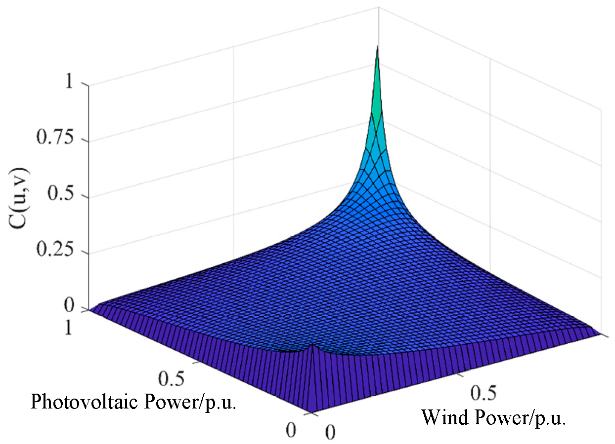
5.1. Select the Optimal Copula Function

Firstly, the marginal distribution functions of wind power and photovoltaic power are obtained based on the non-parametric kernel density estimation method, and then the binary histograms of wind power and photovoltaic power are obtained by calculation, as shown in Figure 5.

According to the obtained binary histogram, using the likelihood estimation method to find that wind power and photovoltaic power are at the edge of the distribution function of the Copula parameter values. Results are shown in

Table 1. Copula function correlation coefficient table.

Copula Function	Clayton	Gumbel	Frank
correlation coefficient	0.5423	1.2763	2.5124

below:

The density function and distribution function graphs of the three functions are shown below (Figure 6, Figure 7 and Figure 8):

According to the three Archimedean Copula functions, the Kendall and Spearman rank correlation coefficients and the squared Euclidean distance d of the three functions and the original data are calculated by the correlation evaluation index formula, and the results are shown in

Table 2. Calculation results of different Copula function evaluation indexes.

Evaluating Indicator	Function Category	Indicator Value
Kendall Rank Correlation Coefficient	Raw Data	0.2432
	Clayton	0.2032
	Frank	0.2453
	Gumbel	0.2216
Spearman Rank Correlation Coefficient	Raw Data	0.4117
	Clayton	0.3254
	Frank	0.4129
	Gumbel	0.3843
Squared Euclidean Distance	Clayton	0.9026
	Frank	0.0715
	Gumbel	1.2036

below:

From the results of the correlation evaluation index, the comprehensive evaluation results of the Frank–Copula function are better, and the best description for the photovoltaic–wind joint power correlation, so in this paper, the Frank–Copula function is selected to establish the photovoltaic–wind joint power model.

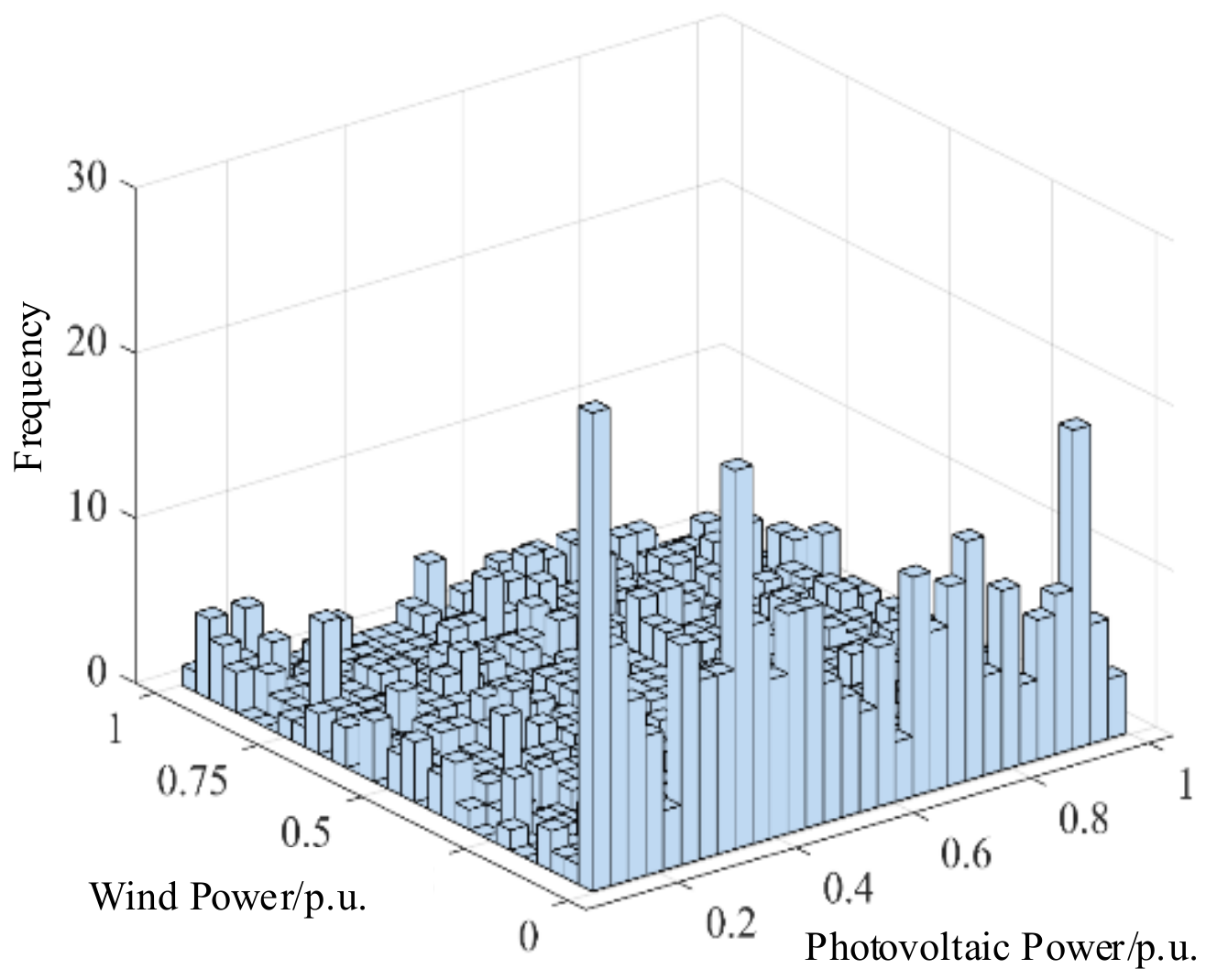
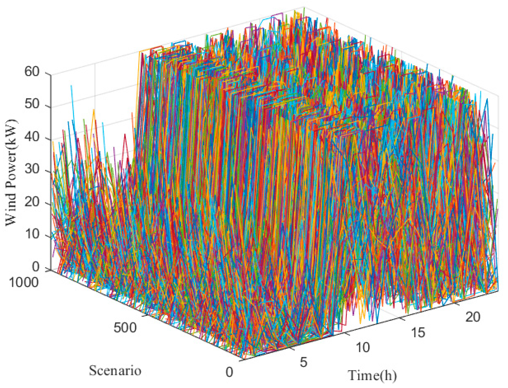
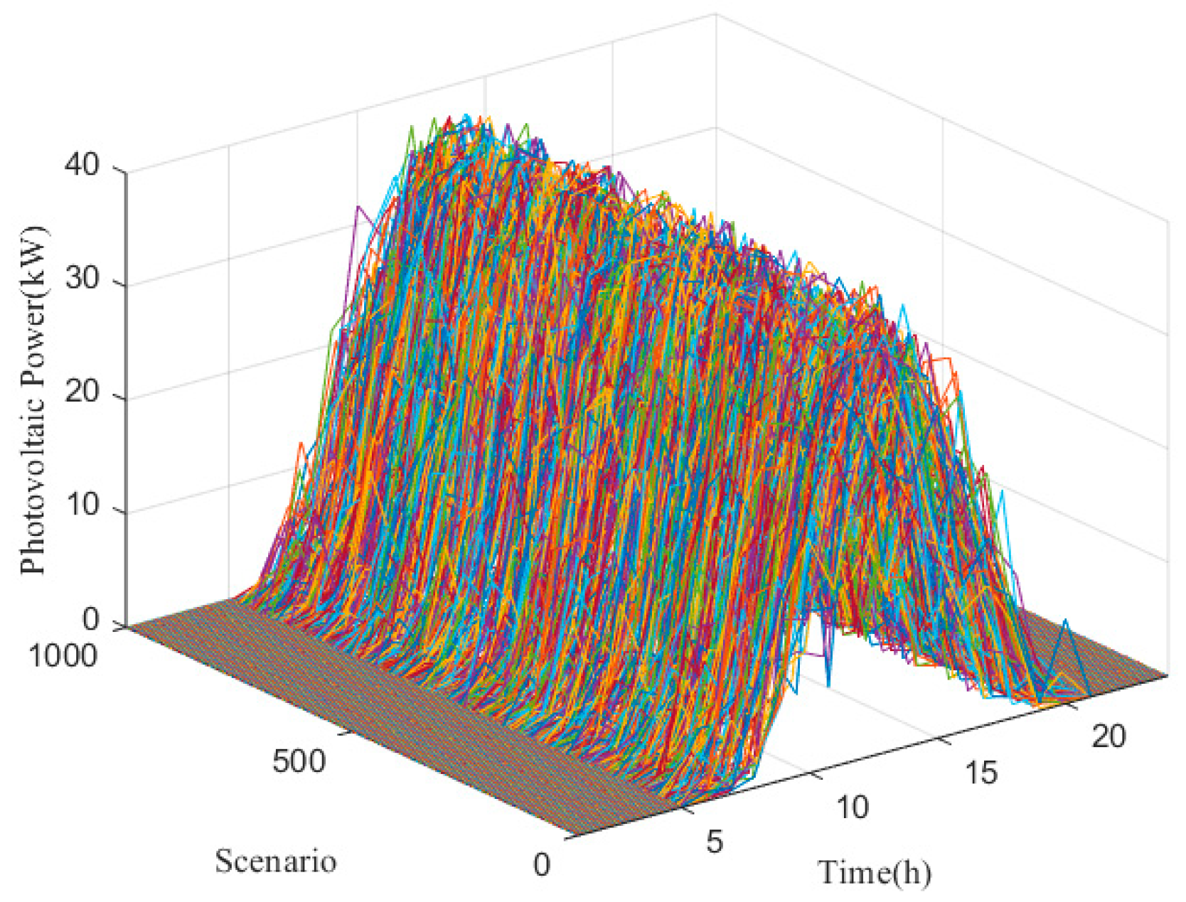
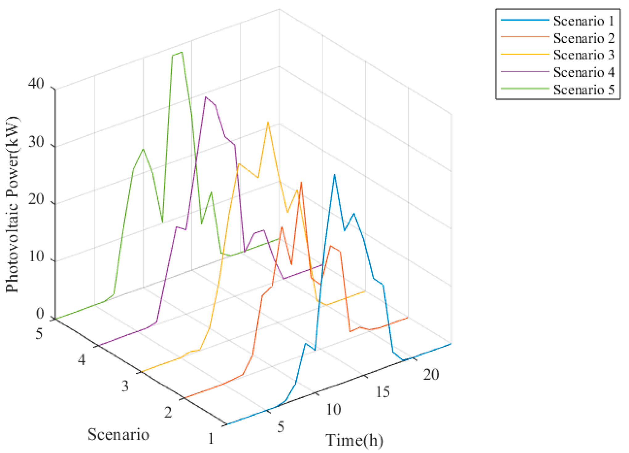
5.2. Joint Output Scenario Generation of Wind and Photovoltaic Power

According to the method described above, first, 1000 wind power photovoltaic output scenarios are generated by sampling from the wind power and photovoltaic Statistical model through the Latin hypercube sampling method. The rated power of the wind turbine is set to 60 kW, and the rated power of the photovoltaic output is set to 40 kW. The generated wind power and photovoltaic original output scenarios are shown in Figure 9 and Figure 10.

From Figure 9 and Figure 10, the generated wind power and photovoltaic energy have strong volatility and randomness output, which conforms to the probability distribution model. In addition, it can be learned from the initial mentioned method that the initial output scenario is reduced to 5 target scenarios. The reduced wind and photovoltaic power scenarios are shown in Figure 11 and Figure 12:

Compared to the scenario diagram before reduction, the output trend of wind and photovoltaic power generation after reduction still retains its original characteristics. During the period from 0:00 to 5:00, wind power generation is relatively strong while photovoltaic power generation is absent. Conversely, from 10:00 to 12:00, photovoltaic power generation compensates for the shortfall in wind power output, indicating a certain degree of complementarity between the two sources. Additionally, the scenario method effectively captures the uncertainty of wind and photovoltaic output through varying probabilities across multiple scenarios, thereby significantly reducing the complexity of subsequent model solutions. The probability of each scenario is shown in Figure 13.

5.3. Model Solving

Taking the IEEE 39 node system including a wind farm and photovoltaic power plant simulation as an example, the scheduling period is set to 24 h with a time granularity of 1 h. The load and new energy demand coefficients $k^1$ and $k^e$ are set at 5% and 25%, respectively. The operational parameters of the thermal power units can be found in reference [29]. The system’s base voltage is 345 kV, with a base power of 100 MVA. The total system load is 4820 kW + j2300 kvar, and the system topology is illustrated in Figure 14. The parameters for the system nodes are detailed in the referenced the references [30]. The algorithm simulation software is Matlab 2021a, running on a Windows 10 operating system, with a hardware platform consisting of an AMD Ryzen 5 5600G at 3.9 GHz and 16 GB of RAM.

To analyze the optimization performance of ADMOFWA, it was compared with MOPSO and MOFWA. The algorithm parameters are set as the same as those in references [31,32], and the number of global Pareto optimal solution sets was set as 50. The optimal compromise solution obtained by comparing the average results of 50 operations is shown in Table 1, and the pareto front of the algorithm is shown in Figure 15. The Pareto frontier of the ADMOFWA is shown in Figure 16. The results obtained by the ADMOFWA are 4.41% better than traditional FWA in terms of fuel cost optimization, and 6.69% better in terms of pollution emission cost optimization. The ADMOFWA performs better in solving multi-objective dynamic environmental and economic scheduling problems, and the results are shown in Table 3 below:

Table 3. Comparison of algorithm results.

Algorithm	Fuel Cost /YUAN	Pollution Discharge /YUAN
MOPSO	2,488,134	286,009
MOFWA	2,387,105	269,570
ADMOFWA	2,281,716	251,538

Table 3. Comparison of algorithm results.

Algorithm	Fuel Cost /YUAN	Pollution Discharge /YUAN
MOPSO	2,488,134	286,009
MOFWA	2,387,105	269,570
ADMOFWA	2,281,716	251,538

6. Conclusions

To address the impact of uncertainty in wind and solar power generation, a Latin hypercube sampling method was employed to generate scenarios, followed by the application of an improved K-means method for scenario reduction. The resulting scenarios effectively capture the characteristics of fluctuations and uncertainties in renewable energy sources while also reducing the complexity of system scheduling. For the uncertainty and correlation of photovoltaic–wind joint power, it can be seen from the correlation evaluation index results that the Frank–Copula function has a better comprehensive evaluation result and the best description of the wind and photovoltaic correlation. Therefore, the Frank–Copula function is selected to establish a wind and photovoltaic joint output model. Subsequently, a DEED model was established with the objectives of minimizing fuel costs and pollution emissions, taking into account the valve point effects of conventional thermal power units, network losses, and ramp rates. To tackle the high-dimensional multi-objective optimization problem, using the IEEE 39 node system scheduling scheme as an example, the initial 1000 wind and photovoltaic scenarios were reduced to five. An adaptive multi-objective fireworks algorithm was then employed, and its performance was compared with MOPSO and MOFWA, demonstrating the superiority of the ADMOFWA, which integrates differential algorithms, in solving such problems.

This article investigates the dynamic economic dispatch problem considering the uncertainty of renewable energy sources and has achieved certain results. Future research will consider the dynamic economic dispatch of clean energy sources such as hydropower and nuclear power.

References

1. Ramírez, V.M.D.; Paz, A.R.; Marín, J.A. Proposal for a Solution to the Environmental Economic Dispatch Problem Using Scilab. In Proceedings of the 2021 IEEE International Autumn Meeting on Power, Electronics and Computing (ROPEC), Ixtapa, Mexico, 10–12 November 2021; pp. 1–6. [Google Scholar]
2. Yin, Q.; Wang, Z.; Sun, T.; Li, W.; Chong, F. Environmental and Economic Dispatch with Photovoltaic and Wind Power. In Proceedings of the 2019 IEEE Sustainable Power and Energy Conference (iSPEC), Beijing, China, 21–23 November 2019; pp. 1108–1112. [Google Scholar]
3. Wei, X.; Xiaoying, Z.; Kun, W.; Wei, C.; Xiaolan, W. Multi-source Coordination and Scheduling Strategy of New Energy with High Proportion of Wind Power, Photovoltaic and Photothermal. In Proceedings of the 2019 4th International Conference on Intelligent Green Building and Smart Grid (IGBSG), Hubei, China, 6–9 September 2019; pp. 661–665. [Google Scholar]
4. Li, X.; Wang, W.; Wang, H.; Wu, J.; Fan, X.; Xu, Q. Dynamic environmental economic dispatch of hybrid renewable energy systems based on tradable green certificates. Energy. 2020, 193, 116699. [Google Scholar] [CrossRef]
5. Sadoudi, S.; Boudour, M.; Kouba, N.E.Y. Optimal Combined Dynamic Economic and Emission Dispatch Including Wind and Photovoltaic Power Systems. In Proceedings of the 2018 International Conference on Electrical Sciences and Technologies in Maghreb (CISTEM), Algiers, Algeria, 28–31 October 2018; pp. 1–6. [Google Scholar]
6. Li, K.P.; Zhang, Z.Y.; Wang, F.; Jiang, L.; Zhang, J.; Yu, Y.; Mi, Z. Stochastic optimization model of capacity configuration for stand-alone microgrid based on scenario simulation using GAN and conditional value at risk. Power Syst. Technol. 2019, 43, 1717–1725. [Google Scholar]
7. Huang, C.; Wang, L.; Lai, L. Data-driven short-term solar irradiance forecasting based on information of neighboring sites. IEEE Trans. Ind. Electron. 2019, 66, 9918–9927. [Google Scholar] [CrossRef]
8. Song, Y.; Li, H. Typical scene generation of wind and photovoltaic power output based on kernel density estimation and Copula function. Electr. Eng. 2022, 23, 56–63. [Google Scholar]
9. Zhu, X.; Jin, H.; Wang, Y. Analysis on dependence structure among photovoltaic power outputs based on combination of copula function and gaussian mixture model. Acta Energiae Solaris Sin. 2019, 40, 1912–1919. [Google Scholar]
10. Xu, J.; Wu, W.; Wang, K.; Li, G. C-Vine pair copula based wind power correlation modelling in probabilistic small signal stability analysis. IEEE/CAA J. Autom. Sin. 2020, 7, 1154–1160. [Google Scholar] [CrossRef]
11. Bai, J.; Wu, X.; Xia, A. An enhanced multi-objective differential evolution algorithm for dynamic environmental economic dispatch of power system with wind power. Energy Sci. Eng. 2020, 9, 316–329. [Google Scholar] [CrossRef]
12. Gherbi, Y.A.; Lakdja, F. Dynamic economic emission dispatch concidering valve point effect and variale active losse using new optimization method. In Proceedings of the 2022 IEEE International Conference on Electrical Sciences and Technologies in Maghreb (CISTEM), Tunis, Tunisia, 26–28 October 2022; pp. 1–6. [Google Scholar]
13. Yang, Z.; Li, K.; Niu, Q.; Xue, Y.; Foley, A. A self-learning TLBO based dynamic economic/environmental dispatch considering multiple plug-in electric vehicle loads. J. Mod. Power Syst. Clean Energy 2014, 2, 298–307. [Google Scholar] [CrossRef]
14. Zhao, H.; Wang, X.; Li, B.; Si, Q.; Zhao, M. Distributionally robust optimaldispatch for multi-community photovoltaic and energy storage system considering energy sharing. Autom. Electr. Powe Syst. 2022, 46, 21–31. [Google Scholar]
15. Ju, L.; Yu, C.; Tan, Z. A two-Stage scheduling optimization model and corresponding solving algorithm for power grid containing wind farm and energy storage system considering demand response. Power Syst. Technol. 2015, 39, 1287–1293. [Google Scholar]
16. Lydia, M.; Kumar, S.S.; Selvakumar, A.I.; Kumar, G.E. Wind resource estimation using wind speed and power curve models. Renew. Energy 2015, 83, 425–434. [Google Scholar] [CrossRef]
17. Sheng, S.; Zhang, L. Economic dispatch of power system considering the prediction error of wind power, solar energy and load. Proc. CSU-EPSA 2017, 9, 80–85. [Google Scholar]
18. Zhou, W.; Lou, C.; Li, Z.; Lu, L.; Yang, H. Current status of research on optimum sizing of stand-alone hybrid solar–wind power generation systems. Appl. Energy 2010, 87, 380–389. [Google Scholar] [CrossRef]
19. Chen, C.; Zhang, Z. Solving dynamic economic dispatch with electric vehicle based on improved heap-based optimizer algorithm. Appl. Res. Comput. 2024, 41, 3032–3037. [Google Scholar]
20. Wu, H.; Qian, S.; Liu, Y.; Xu, G.; Guo, B. Multiobjective dynamic economic emission dispatch differential evolution algorithm based on elites cloning local search. J. Shandong Univ. Eng. Sci. 2021, 51, 11–23. [Google Scholar]
21. Wu, H.; Lin, Y.; Zeng, X.; Qian, S. Adaptive different evolutionary algorithm and its application of dynamic emission economic dispatch problem. Appl. Res. Comput. 2021, 38, 1443–1448+1454. [Google Scholar]
22. Tian, H.; Wang, K.; Yu, B.; Tian, W.; Song, C.; Wu, Z. Optimal planning method for distribution network considering multi-type load and uncertainty of wind and solar. Proc. CSU-EPSA 2021, 33, 144–150. [Google Scholar]
23. Zhang, L.; Wang, X.; Wang, J.; Zheng, Y.; Ma, Q. Bi-level optimization model of inter-regional power dispatch based on regional electricity price. Electrc Power Autom Equip. 2021, 43, 195–201. [Google Scholar]
24. Sheikholeslami, R.; Razavi, S. Progressive Latin Hypercube Sampling: An efficient approach for robust sampling-based analysis of environmental models. Environ. Model. Softw. 2017, 93, 109–126. [Google Scholar] [CrossRef]
25. Li, J.; Lan, F.; Wei, H. A scenario optimal reduction method for wind power time series. IEEE Trans. Power Syst. 2016, 31, 1657–1658. [Google Scholar] [CrossRef]
26. Beirami, A.; Vahidinasab, V.; Shafie-Khah, M.; Catalão, J.P. Multiobjective ray optimization algorithm as a solution strategy for solving non-convex problems: A power generation scheduling case study. Int. J. Electr. Power Energy Syst. 2020, 119, 105967. [Google Scholar] [CrossRef]
27. Zheng, S.; Li, J.; Janecek, A.; Tan, Y. A cooperative framework for fireworks algorithm. IEEE/ACM Trans. Comput. Biol. Bioinform. 2017, 14, 27–41. [Google Scholar] [CrossRef] [PubMed]
28. Jadoun, V.K.; Pandey, V.C.; Gupta, N.; Niazi, K.R.; Swarnkar, A. Integration of renewable energy sources in dynamic economic load dispatch problem using an improved fireworks algorithm. IET Renew. Power Gener. 2018, 12, 1004–1011. [Google Scholar] [CrossRef]
29. Cui, Y.; Zeng, P.; Wang, Z.; Wang, M.; Zhang, J.; Zhao, Y. Multiple time scales scheduling strategy of wind power accommodation considering energy transfer characteristics of carbon capture power plant. Proc. CSEE. 2021, 41, 946–961. [Google Scholar]
30. Attaviriyanupap, P.; Kita, H.; Tanaka, E.; Hasegawa, J. A hybrid EP and SQP for dynamic economic dispatch with nonsmooth fuel cost function. IEEE Trans. Power Syst. 2002, 17, 411–416. [Google Scholar] [CrossRef]
31. Liu, G.; Peng, C.; Xiang, L. Economic-environmental dispatch using improved multi-objective particle swarm optimization. Power Syst. Technol. 2011, 35, 139–144. [Google Scholar]
32. Zare, M.; Narimani, M.R.; Malekpour, M.; Azizipanah-Abarghooee, R.; Terzija, V. Reserve constrained dynamic economic dispatch in multi-area power systems: An improved fireworks algorithm. Int. J. Electr. Power Energy Syst. 2021, 126, 106579. [Google Scholar] [CrossRef]
Figure 1. Initial distribution of fireworks.
Energies 17 06247 g001
Figure 2. The basic fireworks algorithm flowchart.
Energies 17 06247 g002
Figure 4. The photovoltaic–wind joint power throughout the year.
Energies 17 06247 g004
Figure 5. Binary histogram of wind power and photovoltaic power.
Energies 17 06247 g005
Figure 6. Density function of Clayton–Copula.
Energies 17 06247 g006
Figure 7. Density function of Gumbel–Copula.
Energies 17 06247 g007
Figure 8. Density function of Frank–Copula.
Energies 17 06247 g008
Figure 9. Scenarios of initial wind power.
Energies 17 06247 g009
Figure 10. Scenarios of initial photovoltaic power.
Energies 17 06247 g010
Figure 11. Scenarios of reduced wind power.
Energies 17 06247 g011
Figure 12. Scenarios of reduced photovoltaic power.
Energies 17 06247 g012
Figure 13. Output probability of each scenario.
Energies 17 06247 g013
Figure 14. Improved IEEE 39 node system topology structure.
Energies 17 06247 g014
Figure 15. Pareto front of the ADMOFWA.
Energies 17 06247 g015
Figure 16. Pareto front of the ADMOFWA.
Energies 17 06247 g016