Simulations of CO₂ Dissolution in Porous Media Using the Volume-of-Fluid Method

Abstract

Traditional investigations of fluid flow in porous media often rely on a continuum approach, but this method has limitations as it does not account for microscale details. However, recent progress in imaging technology allows us to visualize structures within the porous medium directly. This capability provides a means to confirm and validate continuum relationships. In this study, we present a detailed analysis of the dissolution trapping dynamics that take place when supercritical CO₂ (scCO₂) is injected into a heterogeneous porous medium saturated with brine. We present simulations based on the volume-of-fluid (VOF) method to model the combined behavior of two-phase fluid flow and mass transfer at the pore scale. These simulations are designed to capture the dynamic dissolution of scCO₂ in a brine solution. Based on our simulation results, we have revised the Sherwood correlations: We expanded the correlation between Sherwood and Peclet numbers, revealing how the mobility ratio affects the equation. The expanded correlation gave improved correlations built on the underlying displacement patterns at different mobility ratios. Further, we analyzed the relationship between the Sherwood number, which is based on the Reynolds number, and the Schmidt number. Our regression on free parameters yielded constants similar to those previously reported. Our mass transfer model was compared to experimental models in the literature, showing good agreement for interfacial mass transfer of CO₂ into water. The results of this study provide new perspectives on the application of non-dimensional numbers in large-scale (field-scale) applications, with implications for continuum scale modeling, e.g., in the field of geological storage of CO₂ in saline aquifers.

1. Introduction

Single and multiphase flow in porous media is the underlying foundation for numerous industrial and natural processes. Researchers have addressed porous media flow at different spatial scales, including the pore scale and the continuum scale. Traditionally, the continuum scale was the dominant experimental approach due to limitations in the measurements inside individual pores. However, recent advancements in imaging technology have enabled the scientific community to capture underlying processes within the void space of the porous medium. Additionally, information from pore scale imaging can be used for the validation of numerical models [1,2]. At the continuum scale, we only retain effective properties of the pore scale details [3]. By construction, effective properties do not capture the full pore scale physics. Therefore, they might lose out on details that are significant for continuum scale effects. One approach for retaining more pore-scale physics is multi-scale modeling, which incorporates pore-scale results into the continuum-scale simulations [4].

Both single and multiphase flow might occur coincidentally with the transfer of species. In a single-phase flow situation, the transport of a dissolved species depends on both the flow field and the concentration gradient of the species [5]. In multiphase flow conditions, mass transport may additionally occur from one phase to another, known as an interfacial mass transfer. Interfacial mass transfer across fluid–fluid interfaces in porous media is a special branch of the generalized multi-phase flow. Significant work has been conducted in the past, especially in the field of enhanced hydrocarbon recovery, geological carbon sequestration, geothermal energy production, seasonal storage of natural gas in geologic formations, nuclear waste management, and gas hydrate formation in sediments [6,7,8,9,10,11,12,13,14]. This wide range of applications has spurred considerable efforts in the modeling of interfacial mass transfer [15,16,17,18,19].

Modeling of interfacial mass transfer has been conducted at different length scales, from μm at the pore scale, to $\mathrm{c}\mathrm{m}$ at the continuum scale [20], and up to km at the field scale [3,21,22]. A review of modeling at different scales is given by Agaoglu et al. [17]. Pore-scale investigations are the foundation for the mass transfer process, as the interfaces over which the mass transfer occurs are fully resolved at this scale. This contrasts with modeling on a continuum scale, where only effective mass transfer properties are considered. Moreover, the pore scale approach yields insight into the effect of void space geometry, e.g., relations to pore and grain size distribution [23], fluid distribution in the porous medium [18], mineralogy and wettability of the rock surface [24], etc. Pore-scale modeling of mass transfer has mostly been studied either by use of network modeling [7,19,25] or direct pore-scale simulations [12,26]. Continuum scale modeling uses the concept of representative elementary volume (REV) to define effective parameters [27]. As the mass transfer is scale dependent, any continuum scale approach would need REV size assessment for the effective mass transfer properties [20].

Pore-scale studies reveal fluid flow and interfacial area distribution. Recent studies identified three domains [17]: (1) the capillary domain involves fluid–fluid interfaces within pore bodies; (2) the thin film area, where the wetting phase covers soil particles and is enclosed by a non-wetting phase; (3) the grain surface roughness area, which refers to a thin layer of residual wetting fluid. Accurate study requires methods that capture these domains [28,29]. In pore-scale modeling, the interfacial mass transfer can effectively be considered in the context of a network of pores and throats, within which the fluid interfaces are captured semi-analytically [7,30,31,32]. Such pore network calculations are mainly targeted towards obtaining effective properties for the mesoscale, which can further be upscaled to macroscopic transport properties at the sample level, incorporating effects of pore micro-structure and fluid micro-distribution such as thin films on transport phenomena. At the next scale, known as mesoscale, experiments, and modeling are conducted in cm scale samples, e.g., of subsurface rock samples. Due to the complexity of flow in porous media at this length scale, many studies have developed correlations between the interfacial mass transfer coefficient and system parameters such as characteristic length, median grain size, mass transfer coefficient of the tracer, Reynolds number, residual tracer saturation, water density, and water kinematic viscosity. Field-scale studies inspect the phenomenon from a wider perspective, and therefore may overlook some of the details, which leads to deficiencies in the results. Parker and Park [20] attested that the interfacial mass transfer coefficient derived from mesoscale experiments was not compatible with the field scale coefficient. They stated that absolute and relative permeability differences, as well as flow velocity, are major reasons for this deficiency [33].

Numerous mathematical models have been deployed in the past to enlighten interfacial mass transfer in porous media. These models have been mostly used for contaminant remediation purposes, especially pollution of water resources by non-aqueous phase liquids (NAPL). The modeling efforts can be classified as analytical and numerical methods. The drawback of the analytical models is their oversimplification of the multiphase systems [20,34,35]. Conversely, numerical models can capture the complexities of multiphase systems, but they require more effort to simulate. These models can be classified as pore-scale or continuum-scale models. Pore-scale simulation models such as pore network methods [19,25,36], Lattice–Boltzmann methods [10,12], and volume of fluid methods [26] have been used to quantify interface mass transfer at the mesoscale. In contrast, continuum-scale models represent the interface mass transfer at a continuum scale and can therefore be applied to field-scale studies.

The simplifications made in pore network models to represent the porous medium may result in inaccurate calculations of interfacial area. The Lattice–Boltzmann method is based on the molecular description of the fluid. It is grounded on the Boltzmann equation. Therefore, physical processes can be directly simulated by modeling the interaction between molecules. This method has a simple programming implementation and excellent parallel scalability [37]. Compared to other multiphase flow modeling methods, such as volume of fluid and level set, LBM models capture the interface dynamics and deal with the boundary conditions more effortlessly. The computational fluid dynamics (CFD) method, which is based on solving the Navier–Stokes equation in a discretized domain, is also used for interfacial mass transfer at pore scale. The main challenge in this method is dealing with the concentration jump at the fluid–fluid interface. Haroun et al. [38] introduced a new single-field continuous species transfer (CST) formulation to solve the discrepancy. Maes and Soulaine [26] added a compressive term in the transport equation and managed to improve the CST model by expressively decreasing the numerical error.

CO₂ trapping in saline aquifers happens under different mechanisms: (1) in structural trapping, where cap rocks behave as barriers and stop the upward migration of CO₂, (2) in capillary trapping, where the capillary forces in the pore space of the rock prevent CO₂ migration, (3) in solubility trapping, where CO₂ can dissolve in saline water, increasing the density of the water which leads to convective mixing that safely store the CO₂, and in (4) mineral trapping, where over time, carbon dioxide reacts with minerals in rock formations to create stable carbonates, which convert CO₂ into a solid, reducing its mobility [39]. The efficiency of CO₂ trapping can also be affected by factors such as brine composition [40] and injection methods [41].

In this research, we attempt to enhance our understanding of the dissolution-trapping mechanism of scCO₂, e.g., in saline aquifers during the process of CO₂ sequestration. Our results can contribute to a broader understanding of diverse transport phenomena in porous media, e.g., groundwater contamination, groundwater remediation, and energy storage in geological formations. We explore the interaction between nondimensional numbers, including Sherwood, Reynolds, Peclet, and Schmidt numbers, in evaluating the dissolution trapping of scCO₂ in saline aquifers.

2. Theory and Background

In this paper, interfacial mass transfer at the pore scale will be described using the stagnant film model. In this model, the interface between two fluids is considered a thin film, and the mass transfer occurs inside this film. The film is considered infinitesimally thin, and thereby volume-free. Since there is no volume associated with the film, there is no storage either. As there is no storage, there are no transients inside the film, thus the concentration gradient between the source and the solvent can be assumed to be linear (i.e., a steady-state solution). The fluid–fluid interface is orders of magnitude thinner than the resolution used in our simulation grid. This justifies the assumption of an infinitesimally thin interface in the modeling.

Therefore, the mass flux across the film can be described through a mass transfer coefficient rate [42]:

$$J=k_{f}a(C_s-C)$$

(1)

where $J$ is the interphase mass transfer rate due to dissolution per unit volume of porous media [$\mathrm{k}\mathrm{g}/{\mathrm{m}}^3/\mathrm{s}$], $k_f$ is a mass transfer coefficient [$\mathrm{m}/\mathrm{s}$], $a$ is the interfacial area between the aqueous phase and non-aqueous phase per unit volume of porous media [$1/\mathrm{m}$], $C_s$ is effective solubility of the solute [$\mathrm{k}\mathrm{g}/{\mathrm{m}}^3$], and $C$ is the non-aqueous phase solute concentration in the aqueous phase [$\mathrm{k}\mathrm{g}/{\mathrm{m}}^3$].

One of the challenges in research concerning porous media is the limited ability to directly observe the processes occurring within it. Previous investigations primarily relied on scaled-up mass transfer methods [43,44].

The rate of interphase mass transfer is commonly expressed in terms of the Sherwood number ($Sh$), which is a function of fluid transport and porous media properties. The interfacial mass transfer coefficient, $k_f$, can be expressed as a function of the non-dimensional Sherwood ($Sh$) number defined as [33]:

$$Sh=\frac{k_f{d}_m}{D_m}$$

(2)

where $D_m$ is the molecular diffusion coefficient [${\mathrm{m}}^2/\mathrm{s}$], while $d_m$ is the mean grain diameter of the porous medium [$\mathrm{m}$]. The Sherwood number is derived from continuum scale experiments while assuming a uniform distribution of fluids in the porous medium. However, pore-scale structure properties such as mean grain diameter, pore size distribution, and wettability have indisputable effects on fluid displacement. Therefore, pore-scale investigations can provide an in-depth perspective on the application of Sherwood number in large-scale (field-scale) applications.

Note that conventionally, due to the challenges in experimental detection of the fluid interface, the mass transfer coefficient and interfacial area are considered as lumped parameters within the analysis. Consequently, a combined mass transfer coefficient ($ka$), derived from the product of the mass transfer coefficient ($k$) and the specific interfacial area ($a$), was used. The significant limitation of relying on a combined mass transfer coefficient is the reliance on porous media characteristics, particularly particle size, as the specific interfacial area cannot be excluded. Consequently, in prior research, the mass transfer model was formulated using a modified Sherwood number instead of the conventional Sherwood number:

$${Sh}^{\prime }=\frac{\mathrm{k}\mathrm{a}{d}_m^2}{D_m}$$

(3)

where, as before, $d_m$ is an effective particle size and $D_m$ is the diffusion coefficient of the trapped phase to the flowing phase. In this article, we will differentiate these terms individually by capturing the interfacial area, and thereby provide a more accurate description of the process. The capability of pore-scale investigations in incorporating pore-scale properties can refine the calculated Sherwood number for further use in continuum-based simulations.

3. Mathematical Model

In this research, we tried to clarify the correlation between the Sherwood number and interfacial mass transfer from a bottom-top perspective. We applied direct pore-scale modeling on three different porous media under different flow conditions. The porous media were generated by Particula [45], which generates three-dimensional packings of particles with predetermined size distributions, simulating both spherical and non-spherical particles with regular and irregular shapes. Then, the surface mesh of each packing (stl files) was converted to a binary Cartesian grid. These binary grids were imported into the voxelToFoam module of the poreFoam solver [46] to generate the volume mesh required by the computational fluid dynamics simulator.

3.1. Two-Phase Flow Modeling

The handling of two-phase, multi-component mass transfer at the pore scale was carried out through two sets of equations—the volume-of-fluid (VOF) formulation for the flow of the multi-phase flow, and the concentration equation with a mass transfer at the fluid–fluid interface (and its extended formulation at the solid boundary). The Navier–Stokes equations were solved on a regular grid using the second-order projection method to simulate multi-phase flows. The pressure was found from the divergence of the temporary solution, and the velocity was corrected by adding the gradient of the pressure. The marker function that identifies different fluids was updated differently in various multi-phase simulation methods.

The VOF method uses unified equations for momentum and continuity to represent the movement of fluid phases across the computational domain, linked with the volume fraction ${\alpha }_i$ of phase $i$. The unified equations are given as:

$$\begin{array}{rr}\frac{\nabla (\rho u)}{\partial t}+\nabla \cdot (\rho \mathrm{u}\times \mathrm{u})& =\mu {\nabla }^{2}u-\nabla p+\rho g+F_{st}\\ \end{array}$$

(4)

$$\nabla \cdot \mathrm{u}=0$$

(5)

where $\mathrm{u}$ represents the velocity field, $p$ signifies the pressure field, $\rho$ stands for the fluid density, $\mu$ represents fluid viscosity, and $F_{st}$ denotes the surface tension force, which can be expressed as:

$$F_{st}=\mathsf{\sigma }\mathrm{k}\mathrm{n}\mathsf{\delta }$$

(6)

Here, $\mathsf{\sigma }$ represents interfacial tension, $\mathrm{k}$ denotes interface curvature (computed as $\mathrm{k}=-\nabla .\mathrm{n}$), where $\mathrm{n}$ is the interface normal determined by $\mathrm{n}=\frac{\nabla \alpha }{\left|\nabla \alpha \right|}$, and $\mathsf{\delta }$ is a Dirac delta function positioned on the interface. To incorporate the surface tension effect, it must be converted into a volumetric force. This transformed force can then be applied as a term similar to a body force within the momentum equation. This conversion process is accomplished through the continuum-surface-force (CSF) method developed by Brackbill et al. [47]:

$$F_{st,CSF}=-\mathsf{\sigma }\nabla \cdot \left(\frac{\nabla \alpha }{‖\nabla \alpha ‖}\right)\nabla \alpha$$

(7)

The CSF model can cause inaccuracies when calculating surface tension forces at low capillary numbers (Ca < 0.01) due to unwanted artificial currents. [47,48,49]. Raeni et al. [46] developed a model called the sharp surface force (SSF) to reduce the impact of artificial currents. The SSF model uses smoothed and sharpened indicator functions to calculate the curvature and the Dirac delta function ($\mathsf{\delta }$).

The evolution of the indicator function ${\alpha }_i$ for each phase, where i = 1 or 2, is governed by an advection equation formulated as

$$\frac{\partial {\alpha }_i}{\partial t}+\nabla \cdot \left({\alpha }_i\mathbf{u}\right)-\nabla \cdot ({\alpha }_i(1-{\alpha }_i)u_r)=0$$

(8)

where $u_r$ represents the relative velocity existing between the two phases [50]. The third component in this equation is an artificial compression factor utilized to enhance the sharpness of the interface, thereby improving the precision of the interface representation. Importantly, this extra term exclusively operates within the interface area and does not impact the solution beyond this zone. The indicator function ($\alpha$) is determined at cell centers and extrapolated linearly to solid boundaries. To calculate normal vectors at the interface, the indicator function is smoothed by interpolating values between cell centers ($c$) and faces ($f$):

$${\alpha }_s=C{〈{〈\alpha 〉}_{c\to f}〉}_{c\to f}+(1-C)\alpha$$

(9)

The coefficient $C$ is set to a value of 0.5, as specified by [46]. This modified indicator function, denoted as ${\alpha }_s$, is employed to determine the normal direction at the centers of the grid cells. When dealing with solid boundaries, adjustments are made to the direction of the normal vector at the interface ($n_{sb}$) to accommodate solid adhesion. This correction is carried out as follows:

$$n_{sb}=n_w\cos \theta +s_w\sin \theta$$

(10)

Here, $\theta$ represents the contact angle of the fluid-fluid interface with the solid boundary, while $n_w$ and $s_w$ denote unit vectors normal and tangential to the solid boundary, respectively.

Ultimately, the smoothed surface tension at the central points of the faces is computed as:

$$F_{st,SSF}=\sigma \nabla \cdot \left(\frac{\nabla {\alpha }_s}{‖\nabla {\alpha }_s‖}\right)\nabla {\alpha }_{sh}$$

(11)

Here, ${\alpha }_{sh}$ represents a refined indicator function as defined by Raeini et al. [46] as:

$${\alpha }_{sh}=\frac{1}{1-C_{sh}}\left[\min \left(\max \left(\alpha ,\frac{C_{sh}}{2}\right),1-\frac{C_{sh}}{2}\right)-\frac{C_{sh}}{2}\right]$$

(12)

In our simulations, we set $C_{sh}$ to a value of 0.5, which serves as a sharpening coefficient. When $C_{sh}$ is equal to 0, it returns $\alpha$ (as in the CSF model), and when it is set to 1, it results in an extremely sharp representation of the interface, which is unstable.

3.2. Mass Transfer Modeling

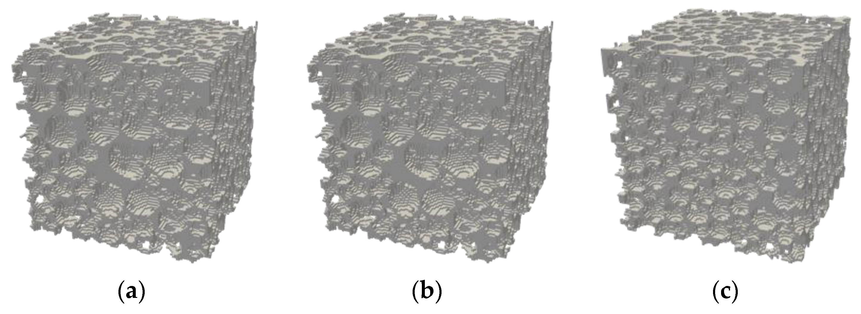
In this section, we outline how chemical mass transfer is incorporated into the VOF framework. We describe the conservation equation for the local concentration $C_{i,k}$ of the chemical species k in each phase $i$:

$$\frac{\partial C_{i,k}}{\partial t}+\nabla \cdot \left(u_i{C}_{i,k}\right)=\nabla \cdot \left(J_{i,k}\right)+R_{i,k}$$

(13)

Here, $u_i$ represents the velocity of phase $i$ locally. $J_{i,k}$ is the diffusion mass flux, determined by Fick’s law and represented as $J_{i,k}=-D_{i,k}\nabla C_{i,k}$, where $D_{i,k}$ is the molecular diffusion coefficient of component $k$ in phase i. In this study, we disregard the reaction term, $R_{i,k}$. The continuity of fluxes and chemical potentials at the fluid–fluid interface is expressed as adherence to the jump condition, as:

$$\begin{gathered} {(C}_{i,k}(u_i-u_I)-D_{i,k}\nabla C_{i,k})\cdot \mathrm{n}=0 \\ {C}_{2,k}=H_k{C}_{1,k} \end{gathered}$$

(14)

Here, $u_I$ is the interface velocity and $H_k$ is Henry’s constant. [51]. When Henry’s law conditions are not met, mass transfer occurs between fluid phases to achieve equilibrium. To simplify, we introduce a global variable for the concentration of species k in a two-phase flow as:

$$C_k=\alpha C_{1,k}+(1-\alpha C_{2,k})$$

(15)

In line with the continuous species transfer (CST) model as introduced by Haroun et al. [38] and Deising et al. [52], the concentration equation within the VOF framework can be expressed as a single-field equation as follows:

$$\begin{gathered} \frac{\partial C_k}{\partial t}+\nabla \cdot \left(u{C}_k\right)=\nabla \cdot \left(D_h\nabla C_k+{\mathsf{\Phi }}_k\right)+R_k \\ {\mathsf{\Phi }}_k=-D_h\frac{C_k\left(1-H_k\right)}{\alpha +H_k\left(1-\alpha \right)}\nabla \alpha \\ {R}_k=\alpha R_{1,k}+(1-\alpha )R_{2,k} \end{gathered}$$

(16)

where $D_h$ is the harmonic mean diffusion coefficient as

$$D_h=\frac{D_1{D}_{2,k}}{{\alpha D}_{2,k}+(1-\alpha )D_{1,k}}$$

(17)

Deising et al. [52] reported that the harmonic mean diffusivity is a more suitable option than the arithmetic mean. In Equation (15), the CST term ${\mathsf{\Phi }}_k$ arises from concentration variations that cause an extra flux at the fluid–fluid interface. This term characterizes the thermodynamic equilibrium at the fluid–fluid interface. When Henry’s coefficient equals one ${(C}_{1,k}=C_{2,k})$, the CST term disappears, resulting in Equation (15) transforming into the standard advection-diffusion equation without the impact of solubility. Maes and Soulaine [26] introduced an enhanced continuous species transfer (C-CST) model by adjusting the advection term within the CST framework. This modification is aimed at improving the accuracy of predictions in situations characterized by high Péclet numbers, where advective mass transfer prevails over diffusion. The C-CST representation of the concentration equation is as follows:

$$\frac{\partial C_k}{\partial t}+\nabla \cdot \left(u{C}_k\right)+\nabla \cdot \left(\frac{C_j-H_j{C}_j}{H_j+\alpha \left(1-H_j\right)}\alpha \left(1-\alpha \right)u_r\right)=\nabla .\left(D_h\nabla C_k+{\mathsf{\Phi }}_k\right)+{\mathrm{R}}_k$$

(18)

Given the demonstrated superior robustness of C-CST compared to the CST framework, we have incorporated it into the VOF framework for simulating species mass transport.

4. Simulations

We utilized the governing equations within the OpenFOAM toolbox to simulate coupled two-phase flow and mass transport [53]. We used interFoam solver in OpenFOAM, equipped with the SSF interfacial tension model, to model two-phase fluid flow. Equation (15) for chemical species conservation was integrated into the GeoChemFoam module by incorporating the hydrodynamics solver with the multicomponent mass transfer model [26].

In our simulations, we generated three distinct sets of densely random-packed grains. These packs consisted of polydisperse grains with no friction. One of these grain packs was composed of non-spherical grains, aiming to represent a real rock sample, while the other two packs were made up of spherical grains. Each pack contained 1000 grains and was enclosed within a cubic container. The grains had a density of $2.65 \mathrm{g}/\mathrm{c}{\mathrm{m}}^3$, which corresponds to quartz minerals, and they exhibited no friction between each other. Figure 1 illustrates the structure of these generated rock samples, while

Table 1. Physical properties of the three rocks.

Rock Sample	Porosity	Permeability (m2)	Voxel Size (μm)	Side Length (m)	Tortuosity	Grain Surface Area (m2)
Realistic rock sample	0.29	$2.82\times {10}^{-12}$	3.0	900	1.22	$3.6474\times {10}^{-5}$
Monodisperse sphere pack	0.34	${5.44\times 10}^{-12}$	3.0	900	1.19	$3.5774\times {10}^{-5}$
Polydisperse sphere pack	0.34	$4.11\times {10}^{-12}$	3.0	900	1.20	$3.9047\times {10}^{-5}$

provides the relevant physical properties of each sample.

In this study, we conducted a sensitivity analysis to examine how fluid properties and flow conditions affect the interfacial mass transfer coefficient. In all our simulations, initially the pore geometries were saturated with water and subsequently injected supercritical carbon dioxide ($\mathrm{s}\mathrm{c}\mathrm{C}{\mathrm{O}}_2$) into the domain to displace the water. We assumed that the pore geometries exhibited a water-wet characteristic with a contact angle of $\theta =45$ degrees. To achieve our target capillary numbers defined as:

$$Ca=\frac{U{\mu }_{co2}}{\sigma }$$

(19)

we adjusted the inlet velocity of the non-wetting $\mathrm{s}\mathrm{c}\mathrm{C}{\mathrm{O}}_2$ (displacing) phase defined as $U$ in Equation (19) accordingly.

Additionally, we varied the diffusivity coefficients of $\mathrm{s}\mathrm{c}\mathrm{C}{\mathrm{O}}_2$ in water to attain different Peclet numbers, defined as the ratio of advective transport rate to diffusive transport rate:

$$Pe=\frac{U{d}_m}{D_m}$$

(20)

where, as before, $d_m$ is an effective grain diameter of the porous medium [$\mathrm{m}$] and $D_m$ is the molecular diffusion coefficient [${\mathrm{m}}^2/\mathrm{s}$]. The Henry coefficient was held constant equal to $0.5$ for all cases. We continued the simulations for several pore volumes beyond the breakthrough of the displacing phase. Figure 2 and Figure 3 illustrate the evolution of saturation and concentration of $\mathrm{s}\mathrm{c}\mathrm{C}{\mathrm{O}}_2$ for each of the rock samples.

To construct the computational grid, we initially formed a background hexahedral mesh covering the entire domain. Then, we eliminated all grid cells located within the solid portion and produced a boundary-fitted mesh by iterative refining and aligning the grid cells with the solid region. The total number of computational grid cells for the realistic rock sample, monodisperse sphere pack, and polydisperse sphere pack after meshing were 305,462, 362,100, and 339,869, respectively. The governing equations for fluid flow and mass transport were discretized using a finite-volume method. These equations were then solved within the pore space of a porous medium to investigate the dissolution of scCO₂ into brine over time.

The pore space was initially saturated with brine and then scCO₂ was injected at a constant flow rate from the left boundary (Figure 3). We maintained a constant pressure condition at the outlet boundary. Additionally, we enforced a no-slip boundary condition at all other boundaries, including the interfaces between the fluid and solid phases. To accommodate the water-wet nature, we specified a receding contact angle $\theta$ of 45 degrees. We set the interfacial tension ($\sigma$) at a value of $34 \mathrm{m}\mathrm{N}/\mathrm{m}$. Initially, we assumed that the brine phase did not contain any dissolved CO₂ (dsCO₂). As we injected scCO₂ from the left boundary, it had the opportunity to dissolve into the brine.

In the current study, we did not consider mineral dissolution or precipitation as a factor. This process typically occurs at a very gradual pace in sandstone reservoirs and becomes significant only over geological timescales [54]. Nevertheless, it is worth noting that certain prior studies have explored the concept of mineral dissolution and its effect on CO₂ trapping, particularly during the injection phase. These findings are more relevant to carbonate reservoirs and have been discussed in studies such as those by Seyyedi et al. [55].

In this study, the influence of the composition of the brine in the aquifer on the dissolution of CO₂ was not considered. The existence of ions in the brine influences the dissolution rate of the CO₂ in the brine as studied by Lin et al. [40].

5. Results and Discussion

We conducted simulations focusing on CO₂ drainage and dissolution to investigate the underlying mechanisms of CO₂ dissolution and mass transfer within a porous medium saturated with brine. The procedure involved injecting supercritical CO₂ into the medium from the left side, with the porous medium initially saturated with brine that was free of dissolved CO₂ (referred to as fresh brine or dsCO₂-free brine, where dsCO₂ indicates the dissolved CO₂ in the brine phase). Through these simulations, we could observe and track the dissolution of CO₂ into the water phase when injecting scCO₂ into the porous medium.

Mobility is a factor that characterizes the flow of a particular phase within a multiphase system. The phase with the greatest mobility will be more mobile and dominate the flow. Mobility is defined as the ratio between the relative permeability of a phase and its viscosity. The simulations were conducted in two different mobility ratios, $M$, defined as the mobility of the displacing fluid (scCO₂) behind the front, ${\lambda }_{\mathrm{s}\mathrm{c}\mathrm{C}\mathrm{o}2}$, divided by the mobility of the displaced fluid (water) ahead of the front, ${\lambda }_w$:

$$M=\frac{{\lambda }_{\mathrm{s}\mathrm{c}\mathrm{C}\mathrm{o}2}}{{\lambda }_w}$$

(21)

The mobility ratios $M=1$ and $M=0.1$ were selected to investigate the effect of fluid dynamics in our study.

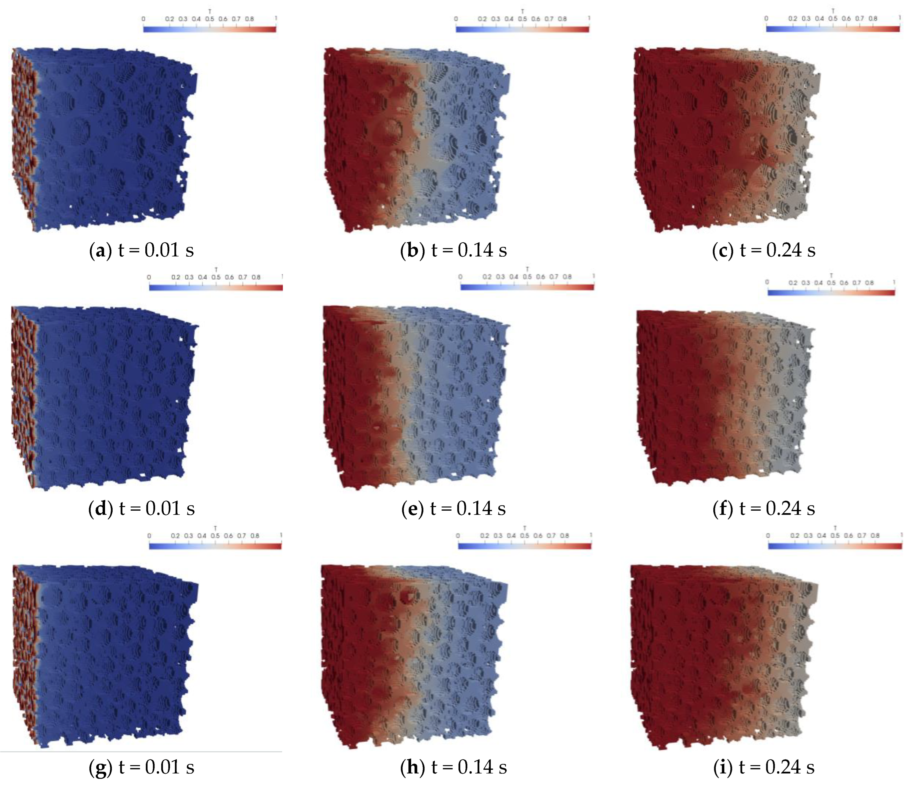
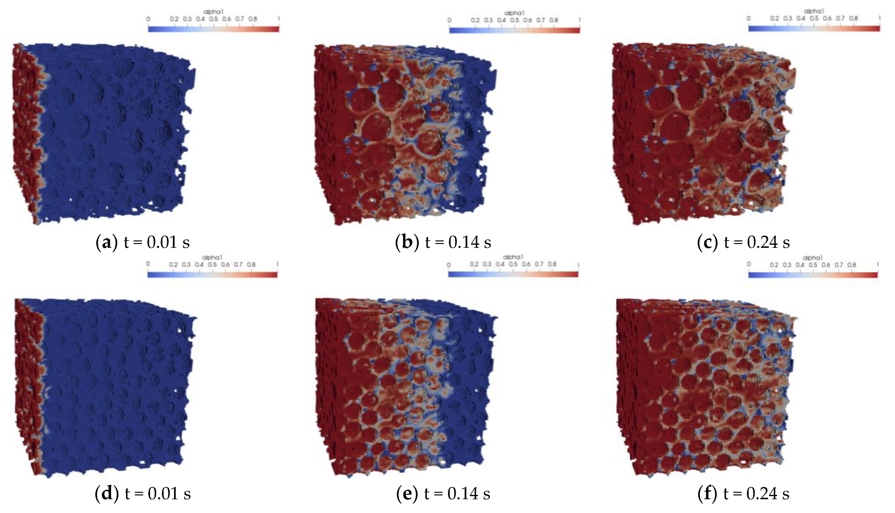
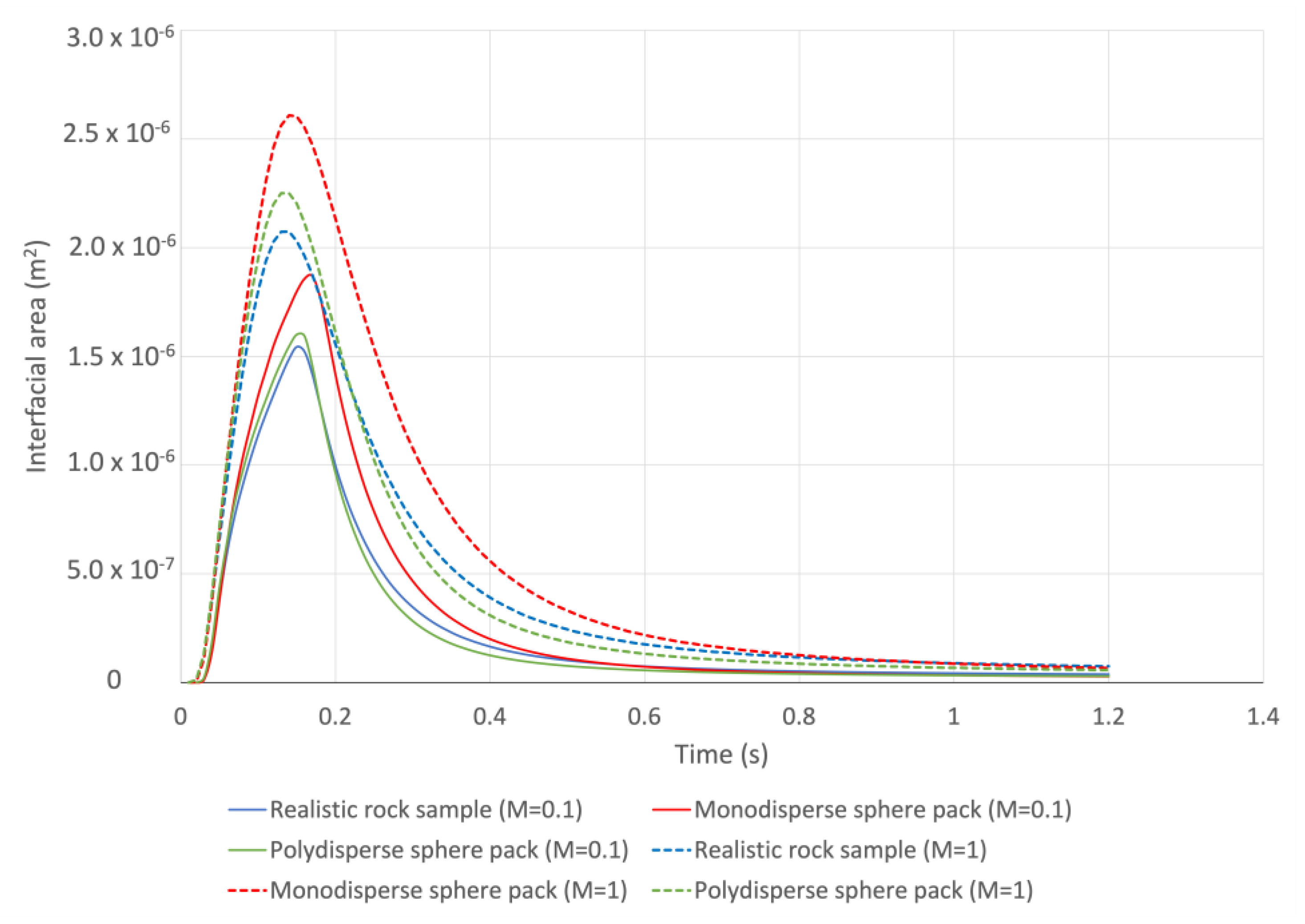
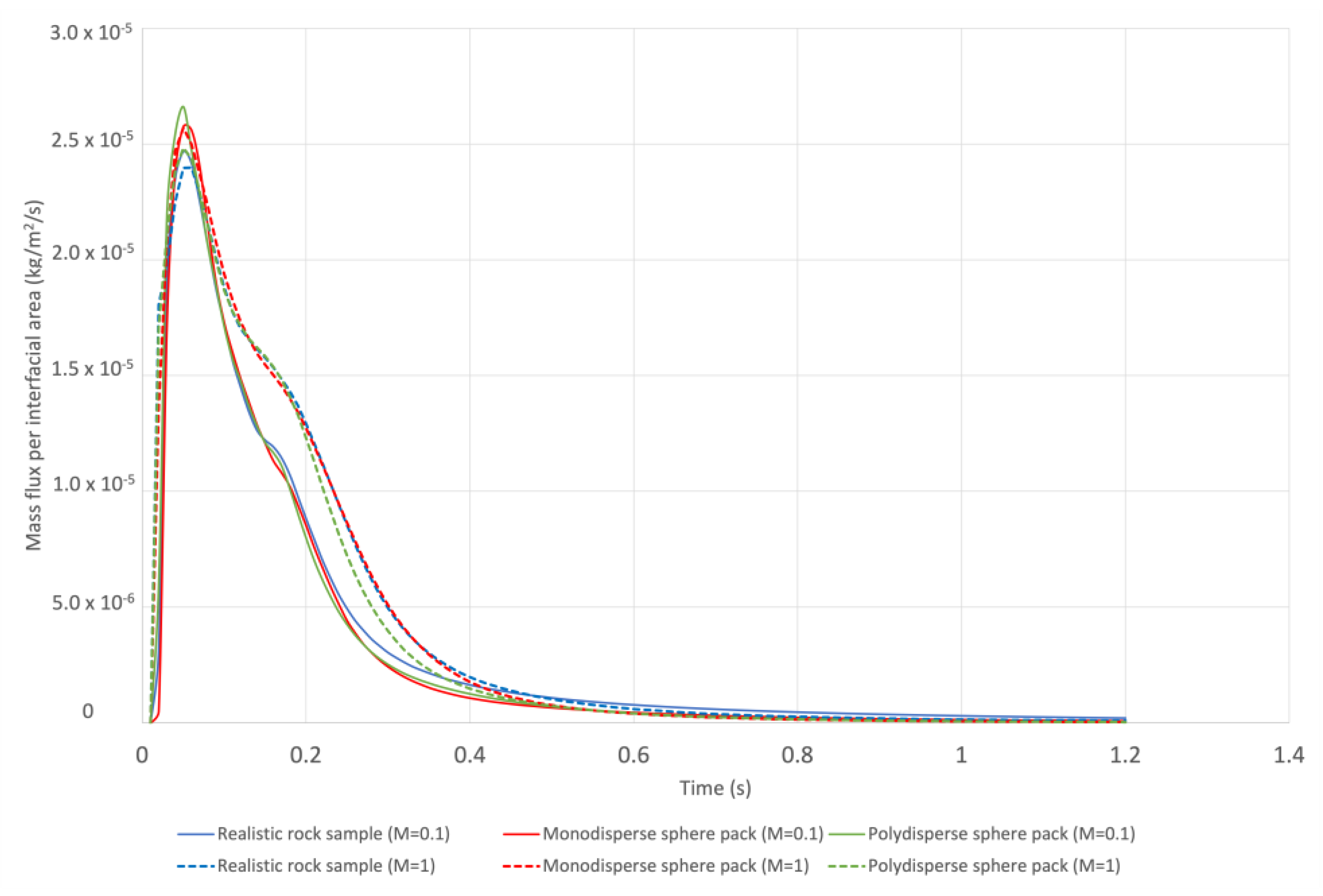
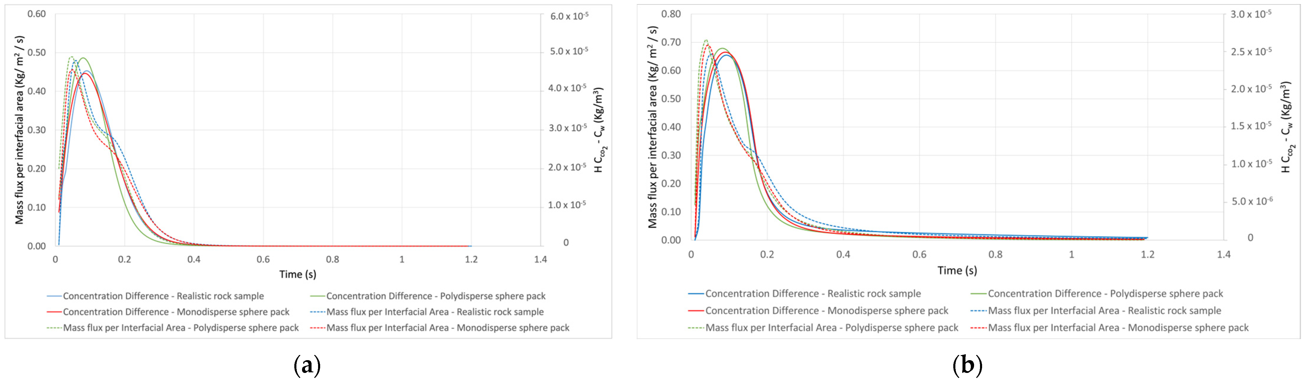
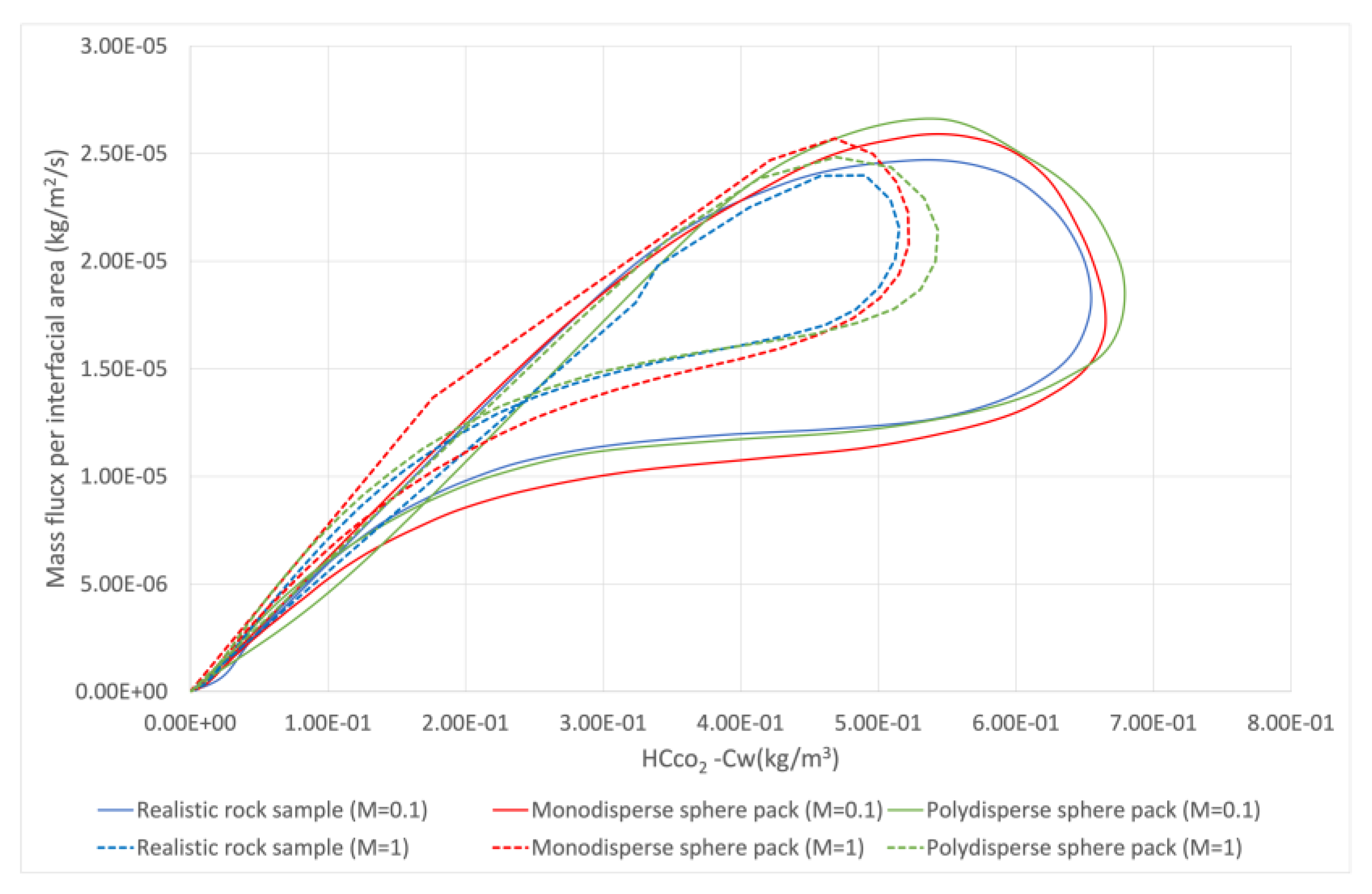
5.1. Analysis of the Simulation Resutlts

The changes in the interfacial area for all our simulations are shown in Figure 4. As we see, the interfacial area for the simulations conducted in $M=1$ was higher than the ones in $M=0.1$. The higher mobility ratio led to more instability of the fluid interfaces, which again led to more viscous fingering and thereby more fluid–fluid interfacial area in the porous medium. Figure 5 displays the mass flux throughout the simulation for each rock sample. The mobility ratio had an impact on the mass flux for all the rock samples, with higher mobility ratios leading to increased mass flux. The mentioned viscous fingering provided the scCO₂ front with a larger fluid–fluid interfacial area, and thereby a greater potential for mass transfer. To account for the impact of the interfacial area on our mass flux results, we depicted the mass flux per interfacial area in Figure 6. We note that the high mobility ratio cases not only had more interfacial area, but also higher mass flux per interfacial area. As mentioned, at high mobility ratio scCO₂ will channel into the medium. We expect the higher mass flux per interfacial area was due to less dissolved CO₂ around the fingers, leading to a higher mass flux.

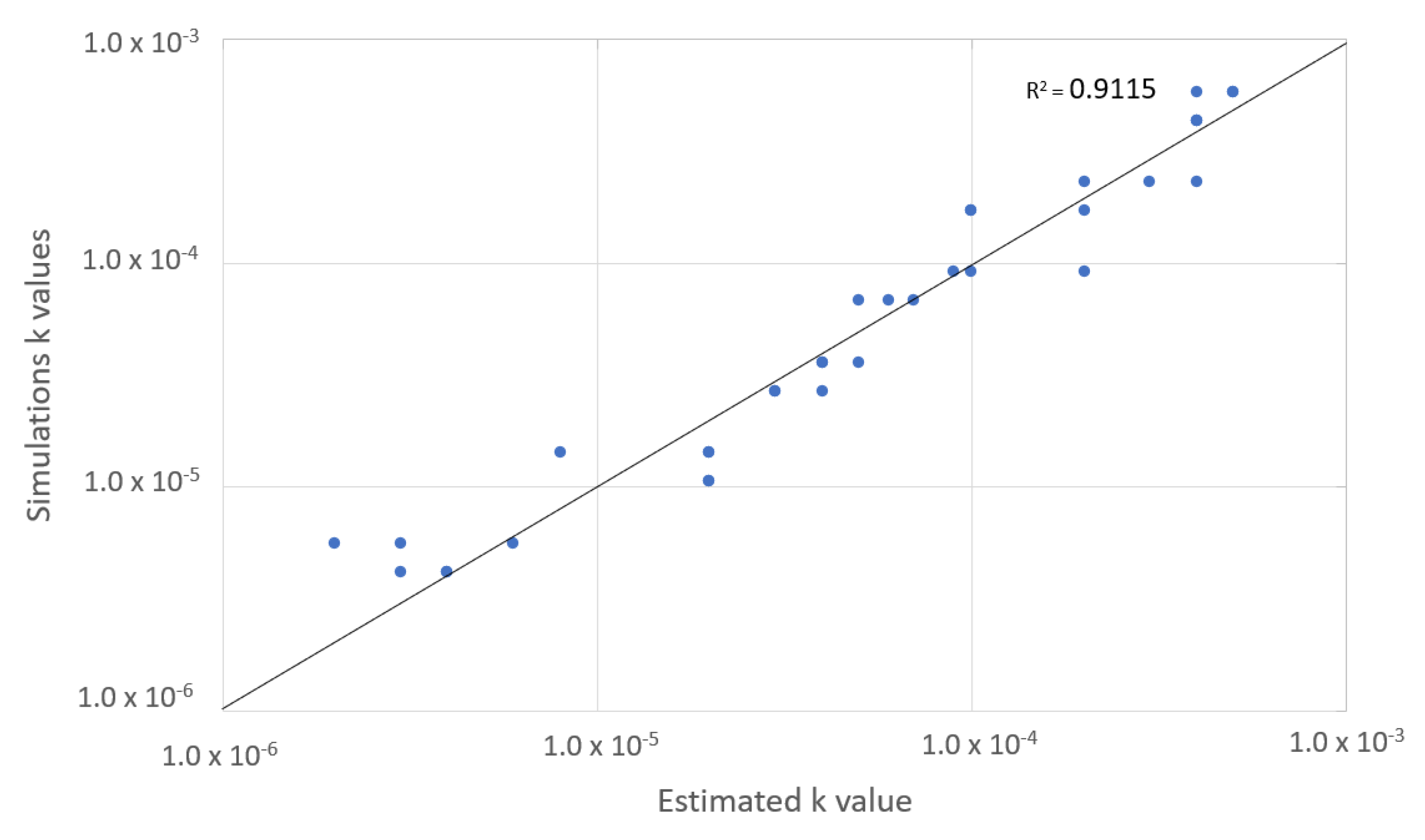
5.2. Estimation of the Mass Transfer Coefficien

In all our simulation cases, there was a strong correlation between mass flux per interfacial area and concentration differences for all rock samples, as depicted in Figure 7. Figure 8 shows how the total mass flux per interfacial area changed as the concentration difference ($H{C}_{co2}-C_w$) varied in all our simulations. For simplification, we investigated the simulations for the realistic rock sample only, which could be generalized to the other simulations. Figure 9 shows the changes in the total mass flux per interfacial area as a function of concentration difference ($H{C}_{co2}-C_w$), during the water drainage by scCO₂ in the realistic rock sample. We notice that, with an equivalent concentration difference, the total mass flux per interfacial area was greater when $M=1$ in comparison to $M=0.1$. In non-equilibrium upscaling models, the interfacial mass transfer coefficient is obtained as the slope of total mass flux per interfacial area versus the concentration difference $H{C}_{co2}-C_w$ [56]:

$${\Phi }^T=k(H{C}_{c{o}_2}-C_w)$$

(22)

where $k$ is the mass exchange coefficient (in $\mathrm{m}/\mathrm{s}$) and ${\Phi }^T$ is the interfacial mass flux.

Following the breakthrough of the scCO₂, it is evident in Figure 8 that the flux can be approximated as linear relative to the concentration difference. The interfacial mass transfer coefficient $(k)$ can subsequently be determined by evaluating the gradient of this function. In Figure 9, considering two different mobility ratios, $M=1$ and $M=0.1$, we derived values of $k=4\times {10}^{-5} \mathrm{m}/\mathrm{s}$ and $k=3\times {10}^{-5} \mathrm{m}/\mathrm{s}$, respectively, for the realistic rock sample. The calculation of the interfacial mass transfer coefficient $(k)$ for the remaining rock samples followed the same procedure.

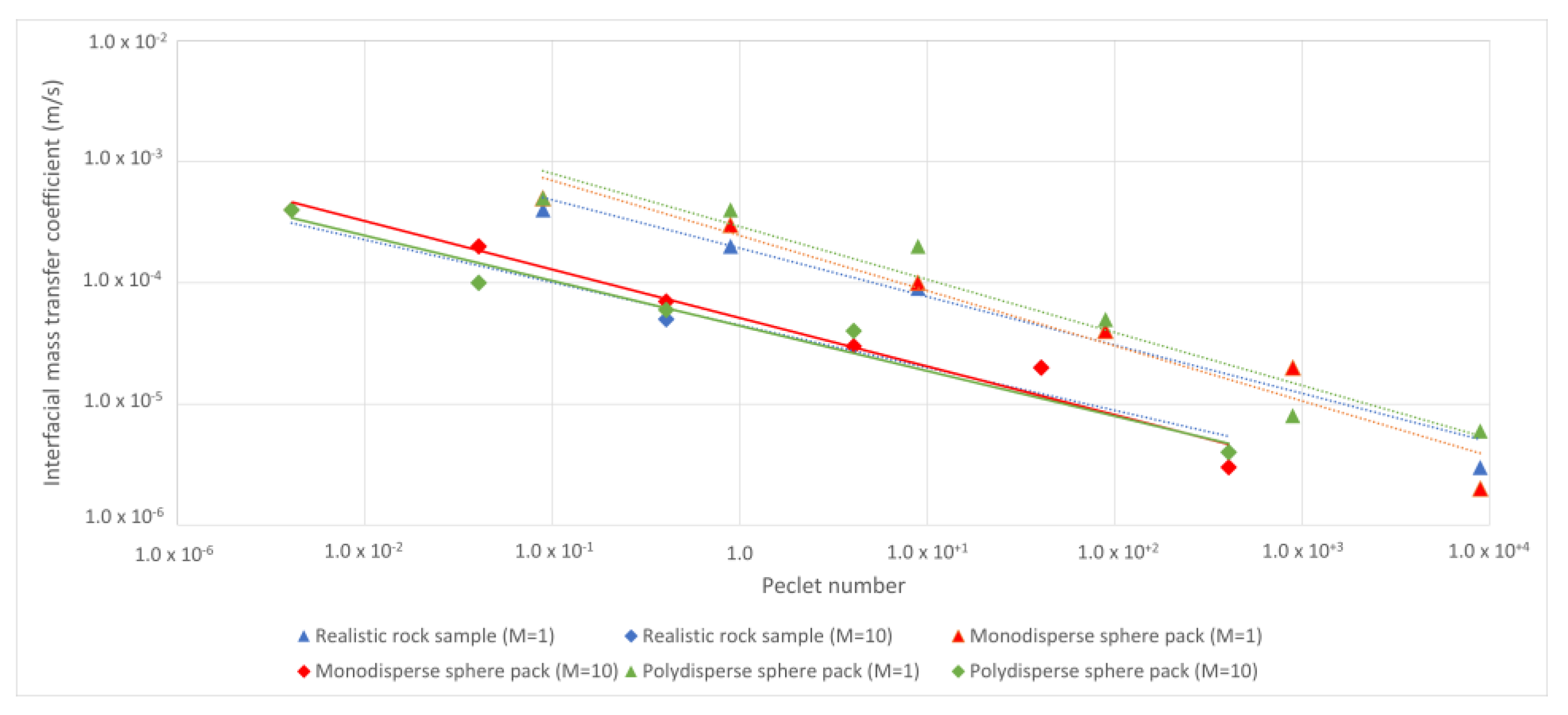
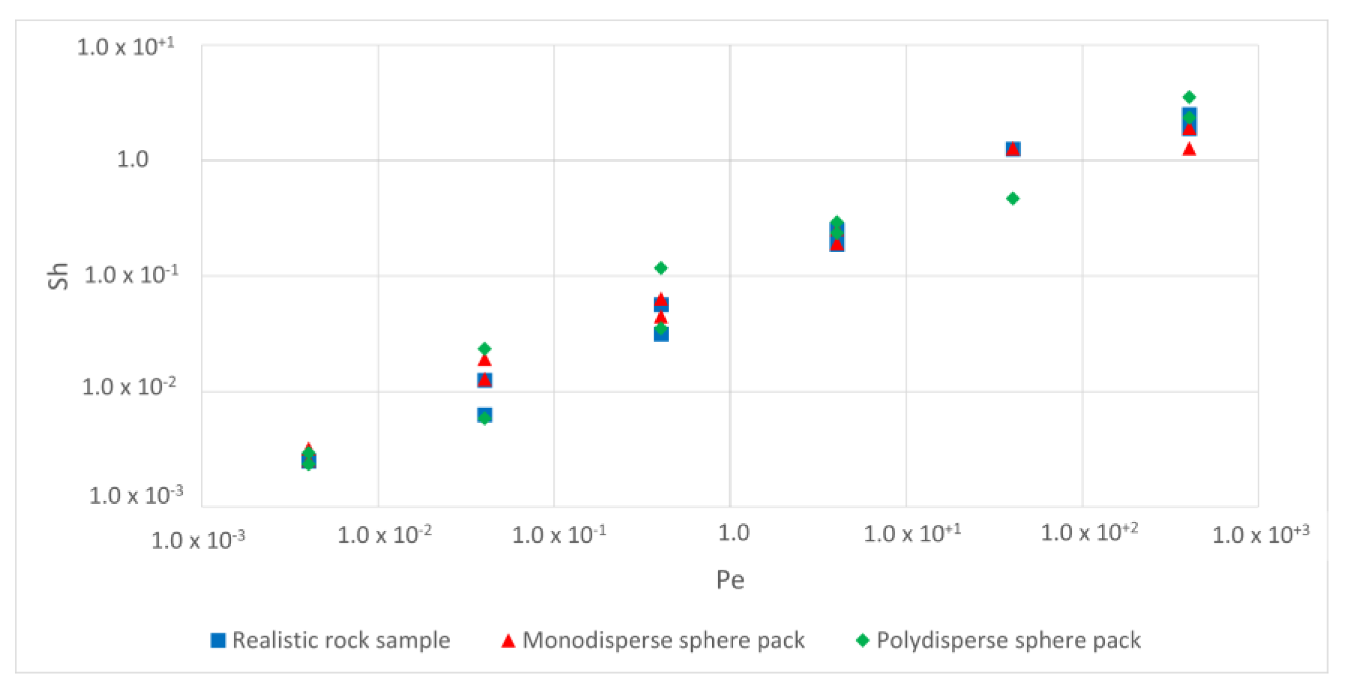
5.3. Development of Sherwood Correlation with Peclet

To explore the relationship between mass exchange coefficients, mobility ratios, and Peclet numbers, the procedure was repeated across a range of diffusion coefficients spanning from ${10}^{-6}$ to ${10}^{-10}$ ${\mathrm{m}}^2/\mathrm{s}$, for both mobility ratios $M=1$ and $M=0.1$. Subsequently, the mass exchange coefficients were plotted against the Peclet number on a logarithmic scale in Figure 10. The equations extracted from the trend line in Figure 10 are reported in

Table 2. The equations and corresponding R-squared values extracted from each of the trendlines in Figure 10.

Rock Sample	M = 1	M = 0.1
Realistic rock sample	$k=2\times {10}^{-4}P{e}^{-0.3999}$ $R^2=0.989$	$k=4\times {10}^{-5}P{e}^{-0.352}$ $R^2=$ 0.9572
Monodisperse sphere pack	$k=2\times {10}^{-4}P{e}^{-0.455}$ $R^2=$ 0.9431	$k=5\times {10}^{-5}P{e}^{-0.4}$ $R^2=0.9899$
Polydisperse sphere pack	$k=3\times {10}^{-4}P{e}^{-0.437}$ $R^2=$ 0.8156	$k=4\times {10}^{-5}P{e}^{-0.372}$ $R^2=0.9614$

. Based on the extracted equations, we see a clear effect of the mobility ratio: in the log–log plot there was a shift in intercept value, while the slope was fairly constant. This implies that the mobility should affect the multiplier in a function of interfacial mass transfer as a function of Peclet number. Therefore, we propose a generalized equation that describes interfacial mass transfer ($k$) as a function of Peclet number (Pe) including the mobility ratio ($M$) as:

$$k={\psi }_1\times M^{{\psi }_2}\times {Pe}^{{\psi }_3}$$

(23)

where ${\psi }_1,$ ${\psi }_2,$ and ${\psi }_3$ are constants and $M$ is the mobility ratio. We used a simple regression to estimate the free variables in Equation (23) and obtained the values ${\psi }_1=6.29\times {10}^{-5}$, ${\psi }_2=-0.402$, and ${\psi }_3=0.128$. Thus, for our simulated data we have:

$$k=6.29\times {10}^{-5}\times M^{0.128}\times {Pe}^{-0.402}$$

(24)

In Figure 11 we have plotted the correlation between the extracted mass transfer coefficients from the simulation results versus the values given by Equation (24). The correlation is good, indicating the predictivity of our proposed equation.

Mass transfer is inherently a phenomenon that depends on the characteristics of the specific system in question. A practical approach for making experimental and small-scale numerical data more universally applicable is to represent them in a dimensionless style and establish relationships between the ratios of forces that impact the system. This allows us to predict that a system operating at a different scale but with equivalent force ratios is likely to yield comparable outcomes. Utilizing our correlation between the interfacial mass transfer coefficient and the Peclet number, we can replace the interfacial mass transfer coefficient from Equation (2) with the one in Equation (23), resulting in an equation for the Sherwood number as a function of mobility ratio (M), the Peclet number (Pe), the mean grain diameter of the porous medium ($d_m$), and the molecular diffusion coefficient ${(D}_m$).

$$Sh={\psi }_1\times M^{{\psi }_2}\times {Pe}^{{\psi }_3}\frac{d_m}{D_m}$$

(25)

By replacing the $d_m/D_m$ in Equation (25) with the one in the Peclet number definition (Equation (20)), we obtain the below equation:

$$Sh=\frac{{\psi }_1\times M^{{\psi }_2}\times {Pe}^{{(1+\psi }_3)}}{U}$$

(26)

We carried out our simulations using a velocity of $U=0.004 (\mathrm{m}/\mathrm{s})$s. Considering the orders of magnitude of the constant values, mobility ratio, and velocity in Equation (26), we have a constant value approximately in the order of 1 × 10⁻².

For comparison, we tried to identify distinctive correlations between the Sherwood and Peclet numbers for each of the rock samples for our simulation results. Hence, we plotted the Sherwood number as a function of the Peclet number in Figure 12. The equations extracted for each of the rocks are shown in

Table 3. Sherwood as a function of Peclet for each of the rock samples.

Rock Sample	Realistic Rock Sample	Monodisperse Sphere Pack	Polydisperse Sphere Pack
$d_m(m)$	$6.28\times {10}^{-5}$	$6.40\times {10}^{-5}$	$5.87\times {10}^{-5}$
Sherwood and Peclet equation	$Sh=0.0779{Pe}^{0.6243}$ $R^2=0.8755$	$Sh=0.0879{Pe}^{0.5727}$ $R^2=0.7462$	$Sh=0.0848{Pe}^{0.5984}$ $R^2=0.9434$

. As observed, the constants in the equations remain moderately consistent across various rock samples with diverse mean grain diameters. Therefore, we also considered general correlation derived from the trendline encompassing all the data in Figure 12, yielding the following equation with an R-squared value equal to $0.8341$.

$$Sh=0.0833{Pe}^{0.5984}$$

(27)

The constant multiplier value in Equation (27) is similar to (${\psi }_1\times M^{{\psi }_2}/U$), derived in Equation (26). Furthermore, the exponent constant in Equation (27) is also similar to the (${1+\psi }_1$) value we obtained in Equation (26).

Researchers have attempted to experimentally determine a relationship between the Sherwood number and the Peclet number [17,33,42,44]. The multiplier and exponent constants reported in the literature [17,33,44] are in good agreement with our findings. However, they were reported for NAPL interfacial mass transfer.

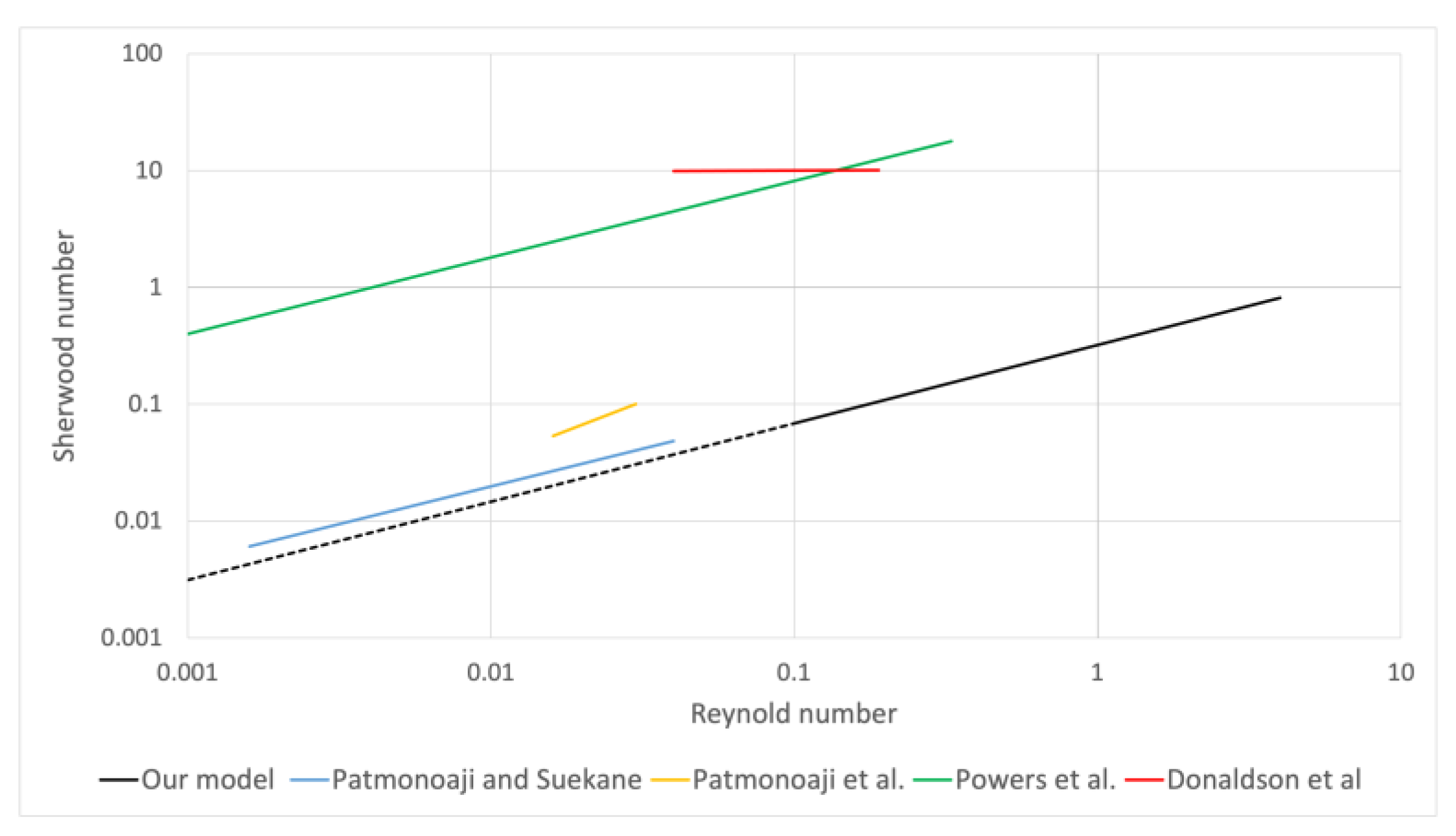
5.4. Development of Sherwood Correlation with Reynold and Schmidt

The Gilliland–Sherwood correlation is a common method for estimating mass transfer coefficient, considering both the stagnant film model and flow conditions:

$$Sh={\phi }_{1}R{e}^{{\phi }_2}S{c}^{{\phi }_3}$$

(28)

where ${\phi }_1$, ${\phi }_2$, and ${\phi }_3$ are considered constants. Within this context, ${\phi }_2$ reflects the relationship between the mass transfer system, fluid flow, and the particle size of the porous media, while ${\phi }_3$ describes the connection between the mass transfer system and the characteristics of both the trapped phase and the flowing phase. Additionally, ${\phi }_1$ accounts for other influencing factors, like the effects of dissolution fingering and two-stage dissolution [57,58,59]. The variable $Re$ is the Reynolds number:

$$Re=\frac{\mathrm{U}{d}_m}{{\nu }_{scCO2}}$$

(29)

where $\mathrm{U}$ is the mean fluid velocity [$\mathrm{m}/\mathrm{s}$], $d_m$ is the geometrical mean diameter of the soil grains [$\mathrm{m}$], $\nu$ is the kinematic viscosity of the displacing phase (scCO₂) [${\mathrm{m}}^2/\mathrm{s}$]. The Reynolds number is a ratio that represents the relationship between the inertia and viscous forces of a moving fluid. The variable $Sc$ is the Schmidt number:

$$Sc=\frac{{\mu }_w}{{{\rho }_{w}D}_m}$$

(30)

The Schmidt number is a dimensionless quantity that compares the momentum diffusivity to the mass diffusivity. By using Equation (31), the mass transfer model for our simulations can be expressed as follows:

$$Sh=0.004R{e}^{0.67}S{c}^{0.577}$$

(31)

The precision of the model is depicted in Figure 13 through a comparison of the Sherwood number obtained from the simulation results on the x-axis with the predicted Sherwood number on the y-axis. As indicated by the black line, this model can also reasonably predict the Sherwood number.

Figure 14 compares our mass transfer model with those previously reported in the literature. Equation (31) was developed for Reynolds numbers between 0.1 and 4 and Schmidt numbers ranging from 0.089 to 8900. In Figure 14, we have presented our model for Schmidt number 2000 as a solid black line. In earlier studies, the interfacial area was difficult to measure experimentally, leading researchers to report the modified Sherwood number instead.

Table 4. Mass transfer models (Sherwood as a function of Reynolds and Schmidt) reported in the literature.

Source	Model	Detail
Patmonoaji and Suekane [57]	$Sh=0.386{Re}^{0.645}$	Schmidt number of trapped CO2 gas at 532 and Reynolds numbers between 0.0016 and 0.04.
Patmonoaji et al. [61]	$Sh=0.337Re$	Schmidt number of trapped N2 gas at 534 and Reynolds numbers between 0.016 and 0.03.
Powers et al. [42]	$Sh=36.8{Re}^{0.654}$	Schmidt number of trapped solid Naphthalene at 1250 and Reynolds numbers between 0.001 and 0.33.
Donaldson et al. [60]	$Sh=2+0.6{Re}^{1/2}+{Sc}^{1/3}$	Schmidt number of trapped solid N2 at 478 and Reynolds numbers between 0.04 and 0.19.

provides a list of previous models that reported the Sherwood number models. The study by Donaldson et al. [60] explored the mass transfer of O₂ in porous media. Under the assumption of uniform sphere distribution equal to particle size, they approximated the interfacial area, and hence, the interfacial area was underestimated. Therefore, their model overestimates the Sherwood number compared to our work. According to our findings, the model created by Powers et al. [42] overestimates the Sherwood number in comparison to our model. Powers model was investigated for a solid–liquid system using naphthalene as the solid phase. This is because there is lower mass transfer in a solid–liquid system, while our model is designed for a scCO₂-water (liquid–liquid) system. The research paper by Patmonoaji et al. [61] proposes a model for a system with gas (N₂) and liquid (water). However, this model overestimates the Sherwood number values. The reason for this could be the difference in the nature of the gas used in their experiment (N₂) compared to ours (scCO₂). The closest model to our proposed model in the literature is given by Patmonoaji and Suekane [57]. Their study investigated mass transfer in a CO₂–water system, and as shown in Figure 14, it is consistent with our model and is widely accepted.

6. Conclusions

We explored the temporary dissolution of scCO₂ as it was injected into porous media saturated with brine, simulating conditions akin to CO₂ geological storage in saline aquifers. Through detailed pore-scale simulations of multiphase and multicomponent flow, we accurately characterized the dynamic distribution of scCO₂ and brine phases, as well as the dissolution process of scCO₂ during the injection phase.

The coefficient governing mass transfer at the interface, necessary for modeling the dissolution rate, is typically described using Sherwood correlations linked to the system’s properties. The primary contribution of this research is an updated Sherwood number, dependent on the Peclet number: we extended the relationship between the Sherwood and Peclet numbers, discovering how the mobility ratio influences the equation. Therefore, we argue that the impact of the mobility ratio should be included in this equation. We have also adjusted the relationship between the Sherwood number, which is based on the Reynolds number and Schmidt number.

Interfacial mass transfer in porous media models is limited due to interfacial area measurement challenges during the dissolution process. For our data, the inclusion of the mobility ratio significantly improved the predictability of mass transfer modeling that omits direct measurements of interfacial area. Our numerically derived mass transfer models based on Sherwood, Reynolds, and Schmidt numbers for the dissolution mass transfer in porous media could improve continuum scale modeling, e.g., modeling the dissolution of scCO₂ in water. We compared our mass transfer model with experimental models reported in the literature and found good agreement for interfacial mass transfer of CO₂ into water.

References

1. Bultreys, T.; Boever, W.; De Cnudde, V. Imaging and image-based fluid transport modeling at the pore scale in geological materials: A practical introduction to the current state-of-the-art. Earth-Sci. Rev. 2016, 155, 93–128. [Google Scholar] [CrossRef]
2. Xiong, T.; Chen, M.; Jin, Y.; Zhang, W.; Shao, H.; Wang, G.; Long, E.; Long, W. A New Multi-Scale Method to Evaluate the Porosity and MICP Curve for Digital Rock of Complex Reservoir. Energies 2023, 16, 7613. [Google Scholar] [CrossRef]
3. Mobile, M.; Widdowson, M.; Stewart, L.; Nyman, J.; Deeb, R.; Kavanaugh, M.; Mercer, J.; Gallagher, D. In-situ determination of field-scale NAPL mass transfer coefficients: Performance, simulation and analysis. J. Contam. Hydrol. 2016, 187, 31–46. [Google Scholar] [CrossRef]
4. Carrillo, F.J.; Bourg, I.C.; Soulaine, C. Multiphase Flow Modelling in Multiscale Porous Media: An Open-Sourced Micro-Continuum Approach. J. Comput. Phys. X 2020, 8, 100073. [Google Scholar] [CrossRef]
5. Icardi, M.; Boccardo, G.; Marchisio, D.L.; Tosco, T.; Sethi, R. Pore-scale simulation of fluid flow and solute dispersion in three-dimensional porous media. Phys. Rev. E 2014, 90, 013032. [Google Scholar] [CrossRef] [PubMed]
6. Chen, L.; Kang, Q.; Robinson, B.A.; He, Y.-L.; Tao, W.-Q. Pore-scale modeling of multiphase reactive transport with phase transitions and dissolution-precipitation processes in closed systems. Phys. Rev. E 2013, 87, 043306. [Google Scholar] [CrossRef]
7. Agaoglu, B.; Scheytt, T.; Copty, N.K. Impact of NAPL architecture on interphase mass transfer: A pore network study. Adv. Water Resour. 2016, 95, 138–151. [Google Scholar] [CrossRef]
8. Niessner, J.; Hassanizadeh, S.M. Modeling Kinetic Interphase Mass Transfer for Two-Phase Flow in Porous Media Including Fluid–Fluid Interfacial Area. Transp. Porous Media 2009, 80, 329. [Google Scholar] [CrossRef]
9. Illangasekare, T.H.; Smits, K.M.; Fučík, R.; Davarzani, H. From Pore to the Field: Upscaling Challenges and Opportunities in Hydrogeological and Land–Atmospheric Systems. In Pore Scale Phenomena; World Scientific Series in Nanoscience and Nanotechnology; World Scientific, 2014; Volume 10, pp. 163–202. [Google Scholar] [CrossRef]
10. Chen, L.; Kang, Q.; Tang, Q.; Robinson, B.A.; He, Y.-L.; Tao, W.-Q. Pore-scale simulation of multicomponent multiphase reactive transport with dissolution and precipitation. Int. J. Heat Mass Transf. 2015, 85, 935–949. [Google Scholar] [CrossRef]
11. Ehlers, W.; Häberle, K. Interfacial Mass Transfer During Gas-Liquid Phase Change in Deformable Porous Media with Heat Transfer. Transp. Porous Media 2016, 114, 525–556. [Google Scholar] [CrossRef]
12. Chen, L.; Wang, M.; Kang, Q.; Tao, W. Pore scale study of multiphase multicomponent reactive transport during CO2 dissolution trapping. Adv. Water Resour. 2018, 116, 208–218. [Google Scholar] [CrossRef]
13. Mwenketishi, G.T.; Benkreira, H.; Rahmanian, N. A Comprehensive Review on Carbon Dioxide Sequestration Methods. Energies 2023, 16, 7971. [Google Scholar] [CrossRef]
14. Pan, X.; Sun, L.; Huo, X.; Feng, C.; Zhang, Z. Research Progress on CO2 Capture, Utilization, and Storage (CCUS) Based on Micro-Nano Fluidics Technology. Energies 2023, 16, 7846. [Google Scholar] [CrossRef]
15. Kokkinaki, A.; O’Carroll, D.M.; Werth, C.J.; Sleep, B.E. An evaluation of Sherwood–Gilland models for NAPL dissolution and their relationship to soil properties. J. Contam. Hydrol. 2013, 155, 87–98. [Google Scholar] [CrossRef] [PubMed]
16. Miller, C.T.; Christakos, G.; Imhoff, P.T.; McBride, J.F.; Pedit, J.A.; Trangenstein, J.A. Multiphase flow and transport modeling in heterogeneous porous media: Challenges and approaches. Adv. Water Resour. 1998, 21, 77–120. [Google Scholar] [CrossRef]
17. Agaoglu, B.; Copty, N.K.; Scheytt, T.; Hinkelmann, R. Interphase mass transfer between fluids in subsurface formations: A review. Adv. Water Resour. 2015, 79, 162–194. [Google Scholar] [CrossRef]
18. Held, R.J.; Celia, M.A. Pore-scale modeling and upscaling of nonaqueous phase liquid mass transfer. Water Resour. Res. 2001, 37, 539–549. [Google Scholar] [CrossRef]
19. Joekar-Niasar, V.; Hassanizadeh, S.M. Analysis of Fundamentals of Two-Phase Flow in Porous Media Using Dynamic Pore-Network Models: A Review. Crit. Rev. Environ. Sci. Technol. 2012, 42, 1895–1976. [Google Scholar] [CrossRef]
20. Parker, J.C.; Park, E. Modeling field-scale dense nonaqueous phase liquid dissolution kinetics in heterogeneous aquifers. Water Resour. Res. 2004, 40. [Google Scholar] [CrossRef]
21. Sainz-Garcia, A.A. Dynamics of Underground Gas Storage. Insights from Numerical Models for Carbon Dioxide and Hydrogen. Ph.D. Thesis, Université Toulouse 3 Paul Sabatier (UT3 Paul Sabatier), Toulouse, France, 2017. [Google Scholar]
22. Brusseau, M.L.; DiFilippo, E.L.; Marble, J.C.; Oostrom, M. Mass-removal and mass-flux-reduction behavior for idealized source zones with hydraulically poorly-accessible immiscible liquid. Chemosphere 2008, 71, 1511–1521. [Google Scholar] [CrossRef]
23. Schnaar, G.; Brusseau, M.L. Pore-Scale Characterization of Organic Immiscible-Liquid Morphology in Natural Porous Media Using Synchrotron X-ray Microtomography. Environ. Sci. Technol. 2005, 39, 8403–8410. [Google Scholar] [CrossRef] [PubMed]
24. Seyedabbasi, M.A.; Farthing, M.W.; Imhoff, P.T.; Miller, C.T. The influence of wettability on NAPL dissolution fingering. Adv. Water Resour. 2008, 31, 1687–1696. [Google Scholar] [CrossRef]
25. Dillard, L.A.; Blunt, M.J. Development of a pore network simulation model to study nonaqueous phase liquid dissolution. Water Resour. Res. 2000, 36, 439–454. [Google Scholar] [CrossRef]
26. Maes, J.; Soulaine, C. A new compressive scheme to simulate species transfer across fluid interfaces using the Volume-Of-Fluid method. Chem. Eng. Sci. 2018, 190, 405–418. [Google Scholar] [CrossRef]
27. Bear, J. Dynamics of Fluids in Porous Media; Dover publications: New York, NY, USA, 1988; ISBN 978-0-486-65675-5. [Google Scholar]
28. Costanza-Robinson, M.S.; Harrold, K.H.; Lieb-Lappen, R.M. X-ray Microtomography Determination of Air−Water Interfacial Area−Water Saturation Relationships in Sandy Porous Media. Environ. Sci. Technol. 2008, 42, 2949–2956. [Google Scholar] [CrossRef] [PubMed]
29. Kim, H.; Rao, P.S.C.; Annable, M.D. Gaseous Tracer Technique for Estimating Air–Water Interfacial Areas and Interface Mobility. Soil Sci. Soc. Am. J. 1999, 63, 1554–1560. [Google Scholar] [CrossRef]
30. Segura, L.A.; Toledo, P.G. Pore-Level Modeling of Isothermal Drying of Pore Networks Accounting for Evaporation, Viscous Flow, and Shrinking. Dry. Technol. 2005, 23, 2007–2019. [Google Scholar] [CrossRef]
31. Wang, Q.; Jia, Z.; Cheng, L.; Li, B.; Jia, P.; Lan, Y.; Dong, D.; Qu, F. Characterization of Flow Parameters in Shale Nano-Porous Media Using Pore Network Model: A Field Example from Shale Oil Reservoir in Songliao Basin, China. Energies 2023, 16, 5424. [Google Scholar] [CrossRef]
32. Luo, C.; Wan, H.; Chen, J.; Huang, X.; Cui, S.; Qin, J.; Yan, Z.; Qiao, D.; Shi, Z. Estimation of 3D Permeability from Pore Network Models Constructed Using 2D Thin-Section Images in Sandstone Reservoirs. Energies 2023, 16, 6976. [Google Scholar] [CrossRef]
33. Sarikurt, D.A.; Gokdemir, C.; Copty, N.K. Sherwood correlation for dissolution of pooled NAPL in porous media. J. Contam. Hydrol. 2017, 206, 67–74. [Google Scholar] [CrossRef]
34. van Genuchten, M.T.; Alves, W.J. Analytical Solutions of the One-Dimensional Convective-Dispersive Solute Transport Equation; United States Department of Agriculture, Economic Research Service: Washington, DC, USA, 1982. [Google Scholar]
35. Hunt, J.R.; Sitar, N.; Udell, K.S. Nonaqueous phase liquid transport and cleanup: 1. Analysis of mechanisms. Water Resour. Res. 1988, 24, 1247–1258. [Google Scholar] [CrossRef]
36. Al-Futaisi, A.; Patzek, T.W. Impact of wettability alteration on two-phase flow characteristics of sandstones: A quasi-static description. Water Resour. Res. 2003, 39. [Google Scholar] [CrossRef]
37. Latt, J.; Malaspinas, O.; Kontaxakis, D.; Parmigiani, A.; Lagrava, D.; Brogi, F.; Belgacem, M.B.; Thorimbert, Y.; Leclaire, S.; Li, S.; et al. Palabos: Parallel Lattice Boltzmann Solver. Comput. Math. Appl. 2021, 81, 334–350. [Google Scholar] [CrossRef]
38. Haroun, Y.; Legendre, D.; Raynal, L. Volume of fluid method for interfacial reactive mass transfer: Application to stable liquid film. Chem. Eng. Sci. 2010, 65, 2896–2909. [Google Scholar] [CrossRef]
39. Benson, S.M.; Bennaceur, K.; Cook, P.; Davison, J.; De Coninck, H.; Farhat, K.; Ramirez, A.; Simbeck, D.; Surles, T.; Verma, P.; et al. Carbon Capture and Storage. In Global Energy Assessment (GEA); Johansson, T.B., Nakicenovic, N., Patwardhan, A., Gomez-Echeverri, L., Eds.; Cambridge University Press: Cambridge, UK, 2012; pp. 993–1068. ISBN 978-0-511-79367-7. [Google Scholar]
40. Liu, B.; Mahmood, B.S.; Mohammadian, E.; Khaksar Manshad, A.; Rosli, N.R.; Ostadhassan, M. Measurement of Solubility of CO2 in NaCl, CaCl2, MgCl2 and MgCl2 + CaCl2 Brines at Temperatures from 298 to 373 K and Pressures up to 20 MPa Using the Potentiometric Titration Method. Energies 2021, 14, 7222. [Google Scholar] [CrossRef]
41. Wang, H.; Kou, Z.; Ji, Z.; Wang, S.; Li, Y.; Jiao, Z.; Johnson, M.; McLaughlin, J.F. Investigation of enhanced CO2 storage in deep saline aquifers by WAG and brine extraction in the Minnelusa sandstone, Wyoming. Energy 2023, 265, 126379. [Google Scholar] [CrossRef]
42. Powers, S.E.; Abriola, L.M.; Dunkin, J.S.; Weber, W.J. Phenomenological models for transient NAPL-water mass-transfer processes. J. Contam. Hydrol. 1994, 16, 1–33. [Google Scholar] [CrossRef]
43. Miller, C.T.; Poirier-McNeil, M.M.; Mayer, A.S. Dissolution of Trapped Nonaqueous Phase Liquids: Mass Transfer Characteristics. Water Resour. Res. 1990, 26, 2783–2796. [Google Scholar] [CrossRef]
44. Powers, S.E.; Abriola, L.M.; Weber, W.J., Jr. An experimental investigation of nonaqueous phase liquid dissolution in saturated subsurface systems: Steady state mass transfer rates. Water Resour. Res. 1992, 28, 2691–2705. [Google Scholar] [CrossRef]
45. Ibrahim, M.A.A.; Kerimov, A.; Mukerji, T.; Mavko, G. Particula: A simulator tool for computational rock physics of granular media. Geophysics 2019, 84, F85–F95. [Google Scholar] [CrossRef]
46. Raeini, A.Q.; Blunt, M.J.; Bijeljic, B. Modelling two-phase flow in porous media at the pore scale using the volume-of-fluid method. J. Comput. Phys. 2012, 231, 5653–5668. [Google Scholar] [CrossRef]
47. Brackbill, J.U.; Kothe, D.B.; Zemach, C. A continuum method for modeling surface tension. J. Comput. Phys. 1992, 100, 335–354. [Google Scholar] [CrossRef]
48. Ubbink, O.; Issa, R.I. A Method for Capturing Sharp Fluid Interfaces on Arbitrary Meshes. J. Comput. Phys. 1999, 153, 26–50. [Google Scholar] [CrossRef]
49. Popinet, S.; Zaleski, S. A front-tracking algorithm for accurate representation of surface tension. Int. J. Numer. Methods Fluids 1999, 30, 775–793. [Google Scholar] [CrossRef]
50. Graveleau, M.; Soulaine, C.; Tchelepi, H.A. Pore-Scale Simulation of Interphase Multicomponent Mass Transfer for Subsurface Flow. Transp. Porous Media 2017, 120, 287–308. [Google Scholar] [CrossRef]
51. Henry, W.; Banks, J. III. Experiments on the quantity of gases absorbed by water, at different temperatures, and under different pressures. Philos. Trans. R. Soc. Lond. 1997, 93, 29–274. [Google Scholar] [CrossRef]
52. Deising, D.; Marschall, H.; Bothe, D. A unified single-field model framework for Volume-Of-Fluid simulations of interfacial species transfer applied to bubbly flows. Chem. Eng. Sci. 2016, 139, 173–195. [Google Scholar] [CrossRef]
53. Jasak, H.; Jemcov, A.; Tuković, Ž. OpenFOAM: A C++ Library for Complex Physics Simulations. 2007. Available online: www.openfoam.org/ (accessed on 23 January 2024).
54. Zhang, D.; Song, J. Mechanisms for Geological Carbon Sequestration. Procedia IUTAM 2014, 10, 319–327. [Google Scholar] [CrossRef]
55. Seyyedi, M.; Mahmud, H.K.B.; Verrall, M.; Giwelli, A.; Esteban, L.; Ghasemiziarani, M.; Clennell, B. Pore Structure Changes Occur During CO2 Injection into Carbonate Reservoirs. Sci. Rep. 2020, 10, 3624. [Google Scholar] [CrossRef]
56. Soulaine, C.; Debenest, G.; Quintard, M. Upscaling multi-component two-phase flow in porous media with partitioning coefficient. Chem. Eng. Sci. 2011, 66, 6180–6192. [Google Scholar] [CrossRef]
57. Patmonoaji, A.; Suekane, T. Investigation of CO2 dissolution via mass transfer inside a porous medium. Adv. Water Resour. 2017, 110, 97–106. [Google Scholar] [CrossRef]
58. Patmonoaji, A.; Hu, Y.; Zhang, C.; Suekane, T.; Patmonoaji, A.; Hu, Y.; Zhang, C.; Suekane, T. Dissolution Mass Transfer of Trapped Phase in Porous Media. In Porous Fluids—Advances in Fluid Flow and Transport Phenomena in Porous Media; IntechOpen: London, UK, 2021; ISBN 978-1-83962-712-5. [Google Scholar]
59. Patmonoaji, A.; Tahta, M.A.; Tuasikal, J.A.; She, Y.; Hu, Y.; Suekane, T. Dissolution mass transfer of trapped gases in porous media: A correlation of Sherwood, Reynolds, and Schmidt numbers. Int. J. Heat Mass Transf. 2023, 205, 123860. [Google Scholar] [CrossRef]
60. Donaldson, J.H.; Istok, J.D.; Humphrey, M.D.; O’Reilly, K.T.; Hawelka, C.A.; Mohr, D.H. Development and Testing of a Kinetic Model for Oxygen Transport in Porous Media in the Presence of Trapped Gas. Groundwater 1997, 35, 270–279. [Google Scholar] [CrossRef]
61. Patmonoaji, A.; Hu, Y.; Nasir, M.; Zhang, C.; Suekane, T. Effects of Dissolution Fingering on Mass Transfer Rate in Three-Dimensional Porous Media. Water Resour. Res. 2021, 57, e2020WR029353. [Google Scholar] [CrossRef]
Figure 1. Pore geometry of the rock samples used in this study: (a) Realistic rock sample; (b) monodisperse sphere pack; (c) polydisperse sphere pack.
Energies 17 00629 g001
Figure 2. Changes in the concentration of dissolved CO2 (red) in the brine phase (blue) over time. The porous medium is assumed to be water-wet with a contact angle of θ = 45°. (ac) Realistic rock sample; (df) monodisperse sphere pack; (gi) polydisperse sphere pack.
Energies 17 00629 g002
Figure 3. Changes in the distribution of the scCO2 phase (red) and the brine phase (blue) within the pore space over time. (ac) Realistic rock sample; (df) monodisperse sphere pack; (gi) polydisperse sphere pack.
Energies 17 00629 g003aEnergies 17 00629 g003b
Figure 4. Changes in interfacial area between the scCO2 and water, during the water drainage by scCO2 in different rock samples.
Energies 17 00629 g004
Figure 5. Evolution of CO2 mass flux from the scCO2 into the water during the water drainage by scCO2 in different rock samples.
Energies 17 00629 g005
Figure 6. Evolution of CO2 mass flux from the scCO2 into the water (as dsCO2) per interfacial area, during the water drainage by scCO2 in different rock samples.
Energies 17 00629 g006
Figure 7. Total mass flux per interfacial area and concentration difference (HCco-Cw) during the displacement mechanism in mobility ratio = 1 (a) and mobility ratio = 0.1 (b).
Energies 17 00629 g007
Figure 8. Changes in the total mass flux per interfacial area, concerning the concentration difference (HCco2-Cw), during the water drainage by scCO2 in different rock samples.
Energies 17 00629 g008
Figure 9. Changes in the total mass flux per interfacial area, concerning the concentration difference (HCco2-Cw), during the water drainage by scCO2 in the realistic rock sample. The triangles on the graphs specify three time steps in the simulations. The inset shows how the interfacial mass transfer was calculated for each of the simulations.
Energies 17 00629 g009
Figure 10. Interfacial mass transfer coefficient (k) measured after the breakthrough of scCO2 versus Peclet number on a log–log scale for all the rock samples.
Energies 17 00629 g010
Figure 11. The correlation between the estimated and the calculated mass transfer coefficients.
Energies 17 00629 g011
Figure 12. The correlation between Sherwood and Peclet numbers for each of the rock samples.
Energies 17 00629 g012
Figure 13. The Sherwood number obtained from the simulation versus the predicted Sherwood number, with the 1-1 line represented by the black line.
Energies 17 00629 g013
Figure 14. Comparison of the mass transfer model developed in this study with other works [42,57,60,61].
Energies 17 00629 g014