Abstract
The air discharge phenomenon, characterized by its rapid and transient nature, is inherently unpredictable, emphasizing the need for a comprehensive understanding of its physical interactions. Our experimental setup involved voltage generators producing both positive and negative impulse voltages (±100 kV, ±125 kV, and ±150 kV) at a 3.5 cm gap distance in a needle-to-plane geometry. This setup facilitated the study of individual spectral lines of impulse voltage discharges, with a specific emphasis on examining oxygen transitions through spectroscopy analysis. To explore the influence of photon emission on the breakdown rate, we examined the correlation between decay time, excitation temperature, and peak intensity during the transition from an upper state to a lower state. Our findings reveal that positive impulse voltage discharges more rapidly than negative impulse voltages. This heightened discharge rate is attributed to the higher peak intensities of O II at 313.421 and 241.162 nm, as well as O IV at 337.806 nm, observed in the excited state, as opposed to O I at 777.417 nm in the combination state. The inference drawn from the larger peak intensity suggests that energetic photon emission plays a pivotal role in initiating and expediting electron discharge in positive voltages.
1. Introduction
A charged object or isolated item will normally gradually lose its charge when surrounded by air because the ambient air serves as an effective insulator. This happens as a result of the atmospheric ions’ limited availability. Ions are mobile charge carriers found in the air. The local ion concentration can, however, rise noticeably in certain circumstances due to the interaction between a charged object and its grounded surroundings. Electrical breakdown is the term for this phenomenon. When a high voltage differential is applied to an insulating material, like air, a localized phenomenon known as breakdown takes place. Typically, an electric field’s effect on the air’s already present mobile charge carriers, such as atmospheric ions and a tiny quantity of free electrons produced by natural decay, is what starts a breakdown. Although free electrons and ions both participate in the random thermal motion of molecules, it is important to remember that their thermal energy is not enough to ionize air molecules through collisions. On the other hand, charged particles in a gas experience acceleration in the electric field and gain more kinetic energy. When the breakdown voltage of the gap is exceeded by the voltage differential between the conductors, gas ionization and a notable decrease in electrical resistance occur, leading to the appearance of a spark.
The short [1,2,3,4,5,6,7,8] and long [9,10] gap distances are two areas of research that are currently very interested in streamer investigations. The discharge under point-to-plane geometry is one of the most interesting geometries for positive discharge in air in observations of short gap distances. A spark breakdown is thought to happen every time with/without a secondary streamer passes through a momentary air gap. Researchers have experimentally investigated the breakdown characteristics using different electrode geometries or configurations, types of applied DC and AC voltages, and gaps of varying lengths in order to uncover breakdown phenomena in air [1,2,9]. They look into extremely irregular electric fields in order to research corona discharges, which can start in the gap prior to a full breakdown (spark) occurring [1,2,3,4,5,6,7,8,9,10]. The Sigmoid [2] stated that the secondary streamer is a secondary indicator of the impending breakdown rather than the primary cause, based on their observation of the initiation breakdown’s characteristics. Additional studies that demonstrate the initiation of a secondary streamer following the primary streamer’s arrival at the grounded plane electrode or its non-arrival prior to the breakdown [1,5] corroborate this hypothesis. After a primary streamer touches the ground, it is thought that the secondary streamer propagates inside the channel, and breakdown happens when the channel that the secondary streamer created heats up [2,6].
The review showed that there were examples where the observations made by different investigators contradicted. The reason for this could be that various researchers focused their research on particular air gaps (such as sphere to sphere, sphere to plane, needle to plane, plane to plane, rod to rod, and rod to plane). Another factor could be the gap length, as well as the material and shape of the electrode. Depending on the generator’s actual connection, even an impulse generator connected to produce the same waveshape may apply a different waveshape to the air gap [7]. It is still difficult to claim a comprehensive understanding of the breakdown process, despite the fact that many theoretical and experimental studies have explained the fundamental discharge process that leads to breakdown, particularly in streamer mechanisms. Since measuring streamer propagation within the nanosecond to picosecond time range is quite challenging, the breakdown mechanism under non-uniform electric fields in the air has not been sufficiently clarified. Furthermore, nothing is known about the breakdown time process.
When examining the electromagnetic emissions that are generated during the discharge process, spectroscopy has been shown to be a valuable instrument. This method allows the light released during a discharge to be separated into its constituent wavelengths. The resulting spectrum provides important information about the physical and chemical conditions, including duration, intensity, and spatial distribution of the light emitted. Our study focused on examining the impact of atomic transitions on the progression of breakdowns in both positive and negative contexts, specifically in relation to the breakdown times. The goal was to gain a deeper understanding of the physical mechanisms characteristic of the breakdown time process. Simplifications and spectroscopy considerations are needed to see the air becoming conductive during the breakdown process. The atomic excitation and relaxation processes following breakdown were investigated in this work using optical measurement. In laboratory experiments, we observed the breakdown time phenomena by choosing the impulse voltage results of ±100 kV, ±125 kV, and ±150 kV in a positive and negative needle-to-plane geometry with a 3.5 cm electrode spacing. After injecting the high-voltage (HV) pulse, an electric field forms across the inter-electrode gap in a positive needle-to-plane geometry. The strongest electric field is seen at the tip of the HV needle electrode, whereas the lowest is at a plane electrode. The strongest electric field’s needle area is where the ionization processes begin, and as a result, free electrons grow exponentially to become avalanches that move in the same direction as the electric field. When the field strength is less than what is needed to accelerate electrons to the gas’s ionization energy, avalanches stop spreading. The exponential growth of free electrons to form avalanches travels in the opposite direction of the electric field in the negative needle-to-plane. Understanding the functions of atomic transitions following breakdown within a less effective electric field depends on this examination of individual spectra. In order to eliminate the effect of electric field propagation, where electrons occupying higher excited orbitals in an excited (or metastable) state remain attached to the atom, the breakdown was thus observed over a significant amount of time, on the order of 10−3 s. An excited atom could be struck by a free electron or absorb additional energy from another photon to become fully ionized. The excited atom would either return to a lower energy state or release a photon, which could excite electrons in another atom if it did not receive any additional energy. To identify the duration phenomena of breakdown, the significance of photon emission results was examined in this study.
2. Experimental Methods
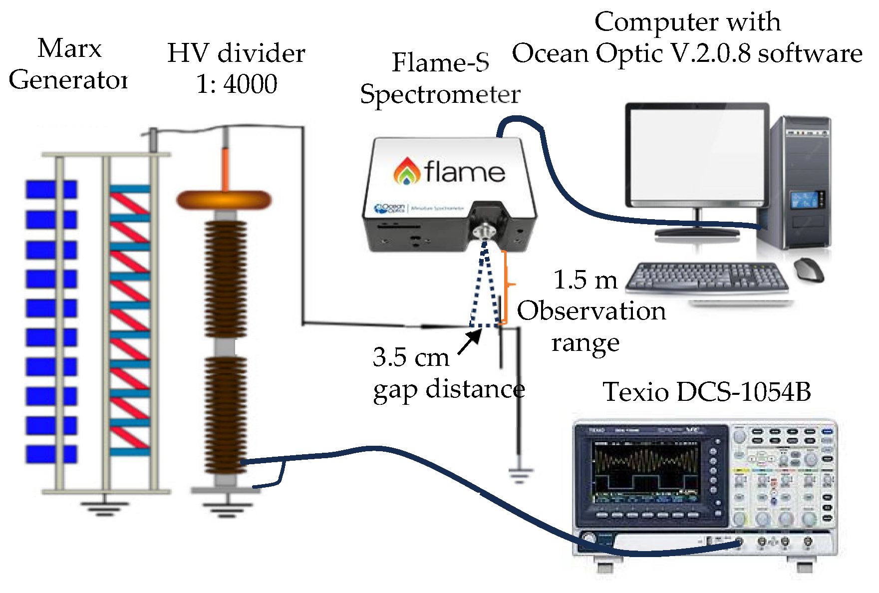
Using high-impulse voltage discharge in both positive and negative configurations, as shown in Figure 1, we examined the optical emission spectra analysis of laboratory-generated high-voltage lightning arcs in this work. A Marx Generator was utilized in our experimental setup as a DC positive and negative impulse voltage source. The voltage options were adjusted to ±100 kV, ±125 kV, and ±150 kV. Two tungsten electrodes were placed horizontally in a needle-to-plane configuration as part of the experimental setup. While the plane electrode stayed grounded, the needle electrode received either positive or negative voltage. A 3.5 cm gap was set as the distance between the electrodes. We used a high-speed oscilloscope, the Texio DCS-1054B, Texio Technology Corporation, Yokohama, Japan, which has a 1 Gbps frequency response and can capture the frequency contents of arc discharge signals to record the impulse voltage signals.

Figure 1.
Experimental platform.
Spatiotemporal capture of spectral lines within milliseconds was essential for investigating the electron transition from an excited state to a lower state, which is how the breakdown process is examined. To achieve this objective, we utilized a Flame-S Ocean Optics spectrometer, Ocean Insight, Orlando, FL, USA, to measure the relative intensity of spectra that are capable of detecting wavelengths ranging from 190 to 1050 nm, with an optical resolution of 1.33 nm (spectral resolution varying from 0.1 to 10 nm). The entrance slit was set at 25 µm, and the scan rate was adjusted to 400 Hz (equivalent to 2.5 ms). By configuring the integration time to 70 ms, we were able to capture spectra within the millisecond range, enabling the collection of a higher number of high-energy photons emitted by the atoms using the spectrometer. The Flame-S spectrometer was connected to a computer equipped with Ocean View software version 2.0.8 to store the datalogger through a USB cable.
To be able to investigate the light emission from a narrow source and see when photon emission appeared during the arc discharge, we carried out the slitless spectrometer technique. With the spectrometer in the field of view between the two electrodes, it was positioned about 1.5 m away from the arc discharge. Arc discharges for positive as well as negative voltage discharges were observed in our experiment within the 200–900 nm wavelength range. Standard temperature and pressure (STP) conditions of 20 °C (293 K) and 101.3 kPa were adopted in our experiments in a dark room to guarantee reliable and consistent data collection on the spectral lines during arc discharges. In this experiment, it is possible to neglect the breakdown voltages’ sensitivity to variations in humidity between 60 and 70%. We then examined the spectral outcomes of the arc discharge in order to identify specific peak spectra of oxygen spectral line productions. We adjusted scans to an average of 1 and boxcar width to 0 to reduce the effect of background radiation before spectral capture. The spectral results were adjusted by subtracting the captured spectral background radiation to minimize the effects of ambient radiation. In an effort to prevent overlapping spectra and accurately estimate atom transition, the Gaussian distribution fitting curve needed to be applied. The NIST database collection can then be used to determine the specific peaks of each spectrum dataset collected during an arc discharge [11]. The spectral findings obtained from these oxygen results were analyzed in this paper.
3. Results
3.1. Breakdown Voltage
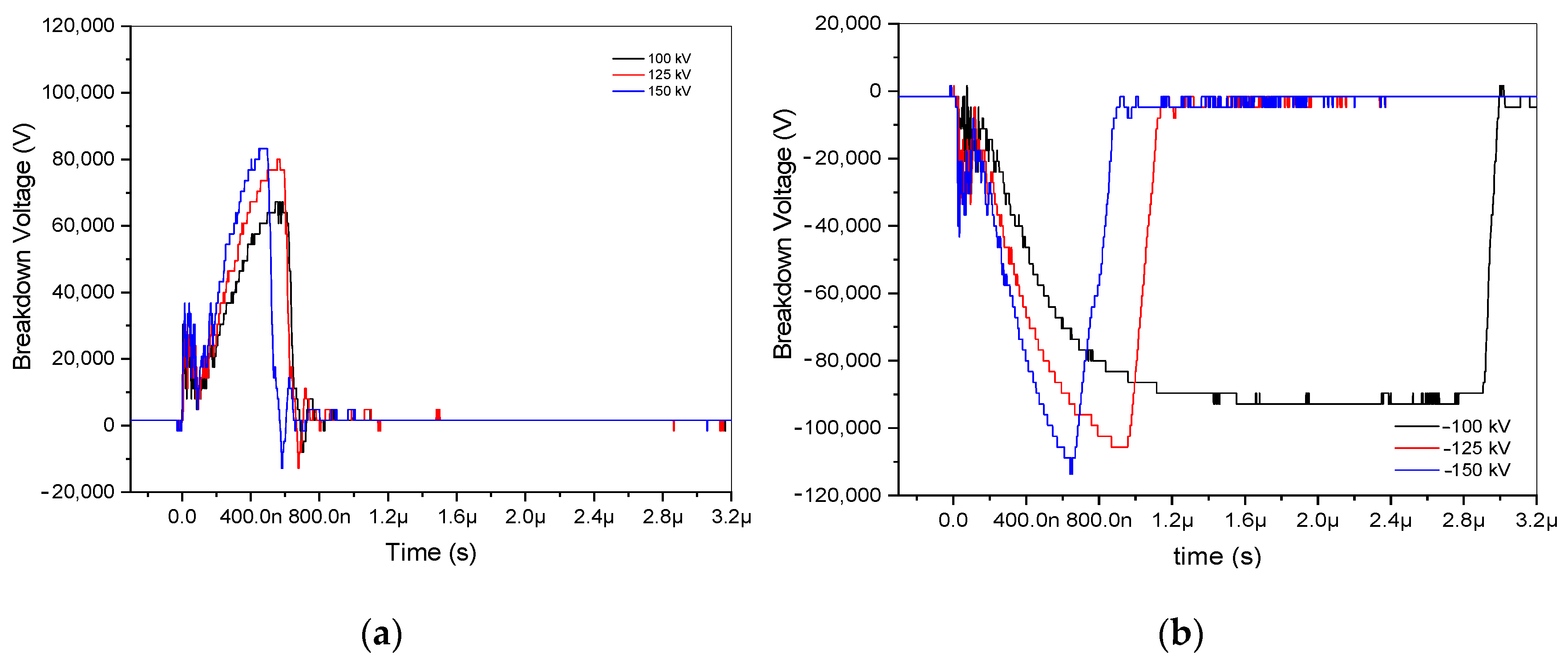
In the experimental analysis, six recordings of positive and negative impulse voltage signals at a 3.5 cm gap were examined. These signals, which included voltages of ±100, ±125, and ±150 kV, were plotted using an oscilloscope. Three positive discharges are arranged, as shown in Figure 2a, and three negative discharges are constructed, as illustrated in Figure 2b. Because it takes an electron that can start an avalanche to build up another one until it reaches the critical charge density, where it forms a low-resistance arc to bridge the gap, the switching time at −100 kV is lengthy. Notably, when the applied voltage ranged from ±100 to ±150 kV, positive voltages demonstrated lower breakdown voltage than negative ones, ranging from 83,200 to 67,200 V and from −113,600 to −92,800 V, respectively. The ±100, ±125, and ±150 kV are represented by the colors black, red, and blue, respectively. Its raised applied voltage results in increasing breakdown voltages. These differences are highlighted in Figure 2, along with different arc discharge durations for positive and negative voltage discharge.
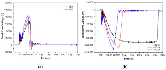
Figure 2.
Breakdown voltage of ±100 kV, ±125 kV, and ±150 kV at a 3.5 gap distance. (a) Breakdown of positive impulse voltage discharge; (b) breakdown of negative impulse voltage discharge.
3.2. Breakdown Time Determination
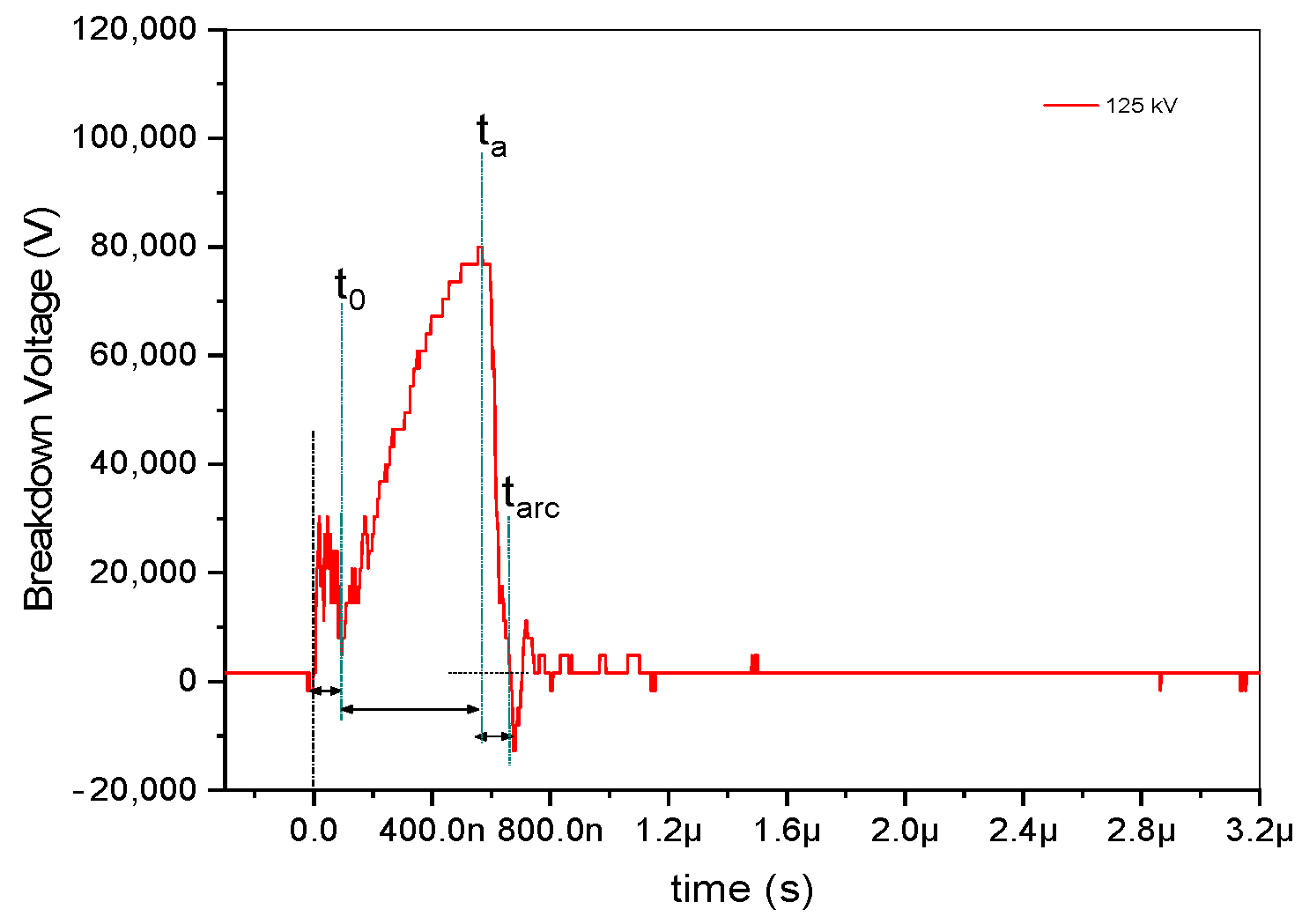
As seen in Figure 3, the impulse voltage waveform is split into four discrete time intervals, each of which provides a role in the development of gas breakdown channels. First, the duration, indicated by the symbol t0, stands for the amount of time it took to reach the static breakdown voltage, which is the lowest voltage needed to cause a breakdown in a non-conductive material when subjected to a static or unchanging electrical field. When the voltage across the material is higher than the static breakdown voltage, the material can no longer withstand the electrical field, which causes current to flow through it and becomes an electrical breakdown [12]. In cases of triggered spark gaps, t0 represents the instant the trigger mechanism is activated.
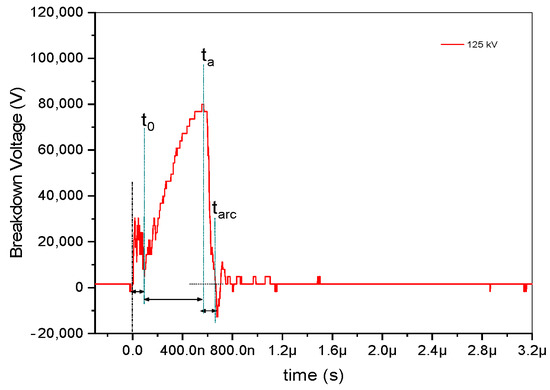
Figure 3.
Time classification determining the dynamics of breakdown in a gas-insulated gap.
The statistical delay time, ts, then signifies the time interval until an electron capable of triggering a presenting avalanche is present. Since the trigger mechanism provides the first necessary electrons, the statistical time lag for triggered spark gaps is typically regarded as insignificant [13]. Moreover, ta is the amount of time required for avalanche buildup until the critical charge density is reached, and tarc is the amount of time required for the formation of a low-resistance arc to bridge the gap. The arc time, denoted as tarc, is derived from the results of positive and negative impulse voltages by subtracting the endpoint of ta time from the endpoint of tarc, as illustrated in Figure 2, and accounting for the applied voltage, as depicted in Figure 3. In the case of negative impulse voltage, a notably shorter arc discharge time of approximately 212 ns was observed at −125 kV. Conversely, in positive voltage, a briefer arc duration of 73 ns was recorded at 150 kV. A fascinating phenomenon is shown in Table 1; the negative impulse voltage tarc has a longer time than the positive impulse voltage tarc by more than twice. The inconsistent tarc duration is seen to occur at the site of negative discharge. In contrast, applied voltages are strengthened by positive impulse voltages, which also decrease the duration of the arc discharge. Consequently, it is necessary to investigate the spectral lines based on examination with respect to the applied voltage at both positive and negative voltages.

Table 1.
The amount of time to bridge the gap for positive and negative voltage discharges.
3.3. Spectral Line Identifications
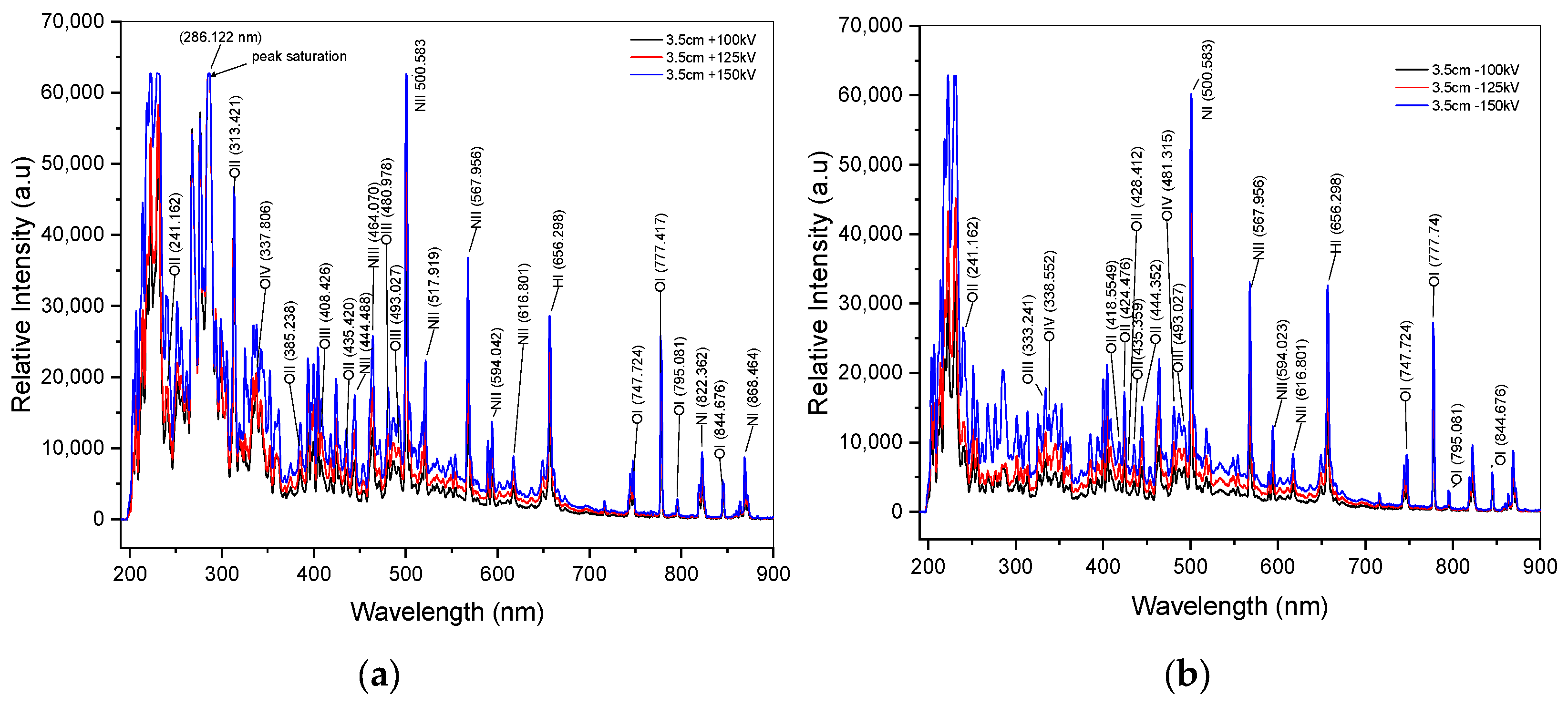
In Figure 4a,b, the recorded spectra by spectrometer from positive and negative impulse voltage discharges are displayed after the onset of arc discharge (breakdown). These spectra mainly exhibit emissions of tungsten, a material for electrode, as well as atomic spectra of dominant elements that are presented in the air such as N, O, H, and Ar. In order to identify individual atoms within these overlapping spectra, we utilized the deconvolution method with Origin 2018 SR1 b9.5.1.195 software for spectral identification. The deconvolution method of fitting curve analysis is essential to minimize the identification of individual atoms from overlapping spectra. For instance, the fitting curve result of a spectral line with a 125 kV range of 308 to 366 nm is presented in Figure 5a, and Figure 5b depicts a spectral line with a −125 kV range of 292 to 318 nm. The excited states of oxygen atoms are represented by the spectral lines in Figure 4a at 125 kV. These lines, which have varying wavelength positions, correspond to singly ionized oxygen (O II), doubly ionized oxygen (O III), and triply ionized oxygen (O IV). Due to the spectrometer’s limited ability to capture photon emission, there are areas of relative peak intensity with saturation values above 63,000 a.u., such as in 125 kV at 286.122 nm for positive impulse voltage, as shown in Figure 4a. The increased intensity emissions from the tungsten electrode during arc discharges are responsible for the saturation value in this band. There is a more energetic intensity of oxygen excited state in positive voltage discharge compared to negative voltage discharge. Overall, all the spectral emissions in both positive and negative impulse voltage in the wavelength range of 500–900 nm yield similar results in the case of the distribution of neutral oxygen atoms. Furthermore, as Section 4.2 illustrates, the relative intensities of the oxygen spectral lines increase proportionately with an increase in applied voltage.

Figure 4.
Spectra of impulse voltage discharge at a 3.5 cm gap distance. (a) Spectra of positive discharge; (b) spectra of negative discharge.
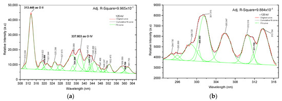
Figure 5.
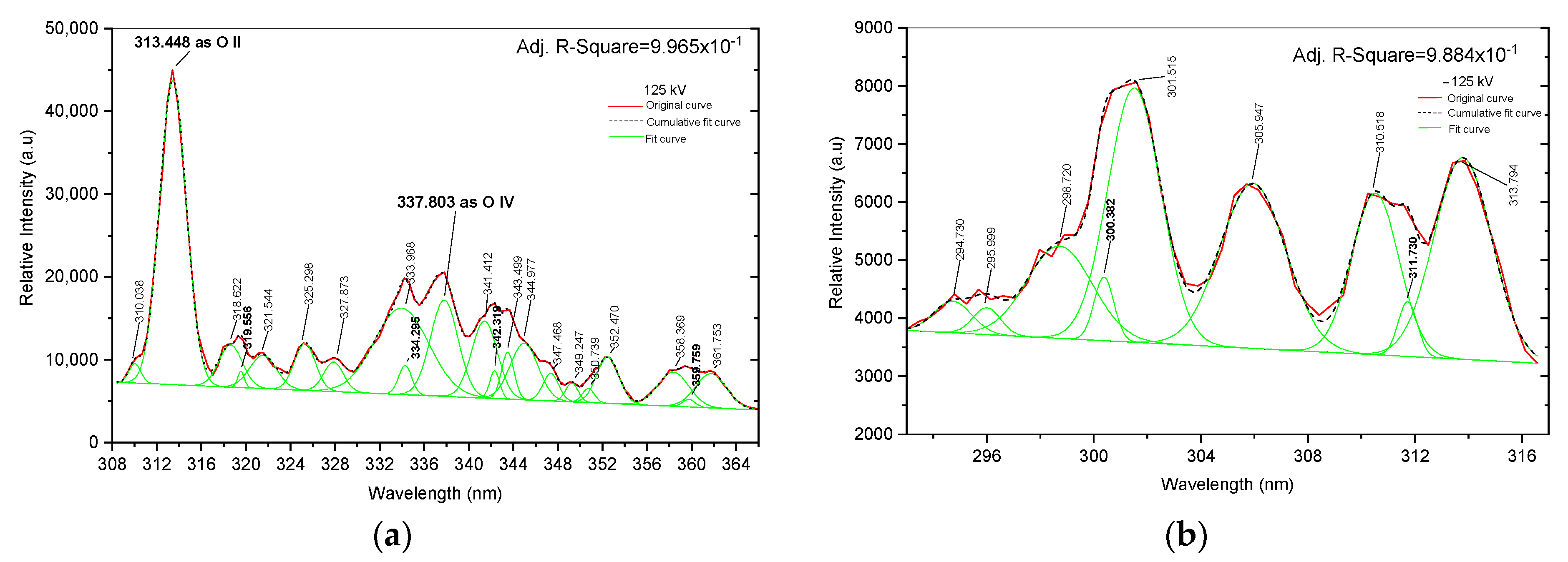
Fitting curve. (a) Positive spectral line from 308 to 366 nm; (b) negative spectral line from 293 to 317 nm.
To ensure the precise identification of individual peak spectra and avoid potential overlap captured by the spectrometer, it is imperative to analyze the fitting curve results using Gaussian distribution through analytical spectral distribution methods. This is demonstrated in Figure 5, where the original curve is represented in solid red, the cumulative curve in dashed green, and the fitted curve in solid green. In Figure 5a, based on an analysis of the NIST data, the individual spectral lines at 313.448 and 337.803 nm are recognized as O II at 313.421 nm and O IV at 337.806 nm, respectively. In Figure 5a at 125 kV, twenty-one prominent peaks indicate various atoms such as argon, nitrogen, and tungsten. The line in the range of 308 to 366 nm describes singly ionized oxygen (O II) at 313.421 nm and triply ionized oxygen (O IV) at 337.806 nm with the correlation factor for this data being 0.996. In contrast, only tungsten is found in the range of 293 to 317 nm in Figure 5b of −125 kV, which shows nine peak indices mainly linked to tungsten atoms and has a correlation factor of 0.988. The spectra of negative voltage discharge in the range of 293 to 317 nm illustrate no spectral lines at 313.421 nm and 337.803 nm, nor do they show any oxygen atoms.
The fitting results, specifically in Table 2, contain detailed information about the identified atomic spectral lines of Figure 5. Therefore, this study specifically focuses on observing individual oxygen spectra transitions in positive and negative impulse voltage discharges, aiming to identify their distinct effects on the duration time to breakdown. Understanding the time to arc for each impulse voltage discharge by observing the physical mechanism of electron production by excitation and recombination of oxygen spectral lines during arc discharge reveals the physical discharge phenomena.
Table 2.
Fitting results for 125 kV and −125 kV of Figure 5.
4. Discussion
4.1. Atomic Distribution and Decay Time
Following the fitting curve, Figure 6a,b illustrates the distribution of oxygen states of arc discharge for both positive and negative impulse voltages. Detailed information on atomic excitation based on NIST data can be obtained in Table 3 and Table 4. The excitation and recombination processes of oxygen atoms play crucial roles in the behavior of breakdown phenomena. It demonstrates that oxygen atoms in an excited state exhibit higher energy excitation in the upper state of O IV, including O III and O II in the wavelength from 200 to 500 nm, as presented in Table 3, denoted as Ek in columns 3 and 7 for positive and negative, respectively. Meanwhile, in the recombination state, O I appears from 500 to 900 nm wavelength range. The excitation energy means that the atom needs the energy to excite to the upper state by absorbing energy and then releasing energy as photon emission in the specific wavelength of its transition. When it falls to a lower state known as recombination energy, indicated by ΔE, as shown in Table 3, signified in columns 4 and 8 for positive and negative, respectively. The oxygen distribution in the 200–900 nm wavelength range is shown in Figure 6a,b for both positive and negative applied voltages corresponding to their intensities. All positive applied voltages exhibit the highest intensity of O II at 313.421 nm and the higher intensity of O II at 241.162 nm relative to O I at 777.417 nm, as can be observed with clarity from the fitting curve results of the spectral lines in Figure 6a,b as well as in Table 3 and Table 4. Moreover, spectral lines of OIV at 337.806 nm, more intense than O I at 777.417 nm, were discovered at positive voltages of 125 kV and 150 kV. O II’s spectral lines at 313.421 and 241.162 nm, as well as OIV’s at 337.806 nm, are more powerful than O I’s at 777.417 nm. In contrast, as illustrates in Table 4, there are no spectral lines of excited states with an intensity greater than O I in any negative voltages. Instead, the intensity displays a random distribution of excited states.
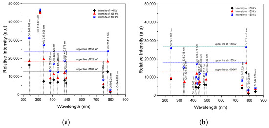
Figure 6.
Distribution of oxygen after fitting curve of ±100 kV, ±125 kV, and ±150 kV applied voltages. (a) Spectra of positive voltage; (b) spectra of negative voltage.
Table 3.
Parameters of oxygen distributions corresponding to NIST.
Table 4.
Parameters of intensity after fitting curve.
The highest peak intensity of neutral oxygen (O I) is shown by the spectral line at 777.417 nm, which is observed in most experimental observations within the wavelength range of 500–900 nm. The observations of oxygen transitioning from an excited state to a neutral state examined the greater intensity of O II at 241.162 nm and 313.421 nm, as well as O IV at 337.806 nm, compared to O I at 777.417 nm. Estimation of the contribution of other parameters in increasing intensity from the upper state to the lower state is estimated using the Boltzmann equation, as follows [14]:
where Iki represents the intensity of the emission, λki is the wavelength of the emitted light, h is Planck’s constant, c is the speed of light in the vacuum, Nk denotes the total population density in the upper state, and Aki signifies the transition probability.
Equation (1) shows that the intensity is directly correlated with energy (ΔE), transition probability (Aki), and the upper state population density (Nk), all of which are listed in Table 3. In the quasi-neutral condition of plasma, the total population density of O II at 241.162 and 313.421 nm, as well as O IV at 337.806 nm, has nearly the same electron density as O I at 777.417 nm. As a result, a higher transition probability, represented by a value of Aki ≫ ΔE, considerably increases the emission intensity. Additionally, as Table 4 illustrates, the increased applied voltage resulted in higher electron densities, which had an impact on spectra’s peak intensity. Table 3 shows that O II at 313.421 nm, 7.68 × 10⁷ s−1, has a higher transition probability in the excited state than the other oxygen atoms at positive voltages, while O II at 418.545 nm, 1.91 × 10⁸ s−1, has a higher transition probability at negative voltages. This suggests that atoms may transition from the upper state to the lower state more quickly due to the higher transition probabilities of O II and O I, which would result in the release of photon energy.
The transition probability can be used to estimate the lifetime of an oxygen atom in the upper state before decaying, which can be used to investigate the rapid impact of O II at 313.421 and 241.162 nm, as well as O IV at 337.806 nm during arc discharge. The lifetime τk of an atomic level k is related to the inverse of transition probabilities as:
τk = 1/Aki
Table 4 presents the lifetime results of the oxygen distribution in positive and negative voltages, which were determined using the data from Table 3. The spectral line of O II at 313.421 nm was found to decay more quickly than other oxygen atoms in the wavelength range of 200 to 900 nm in positive voltage, falling to lower energy levels in a brief period of 1.302 × 10⁻⁸ s. Similarly, the O II line at 418.545 nm has a brief negative voltage duration of 5.236 × 10⁻⁹ s. On the other hand, positive and negative voltages recombine at 2.71 × 10⁻⁸ s.
In contrast to positive voltages, negative voltages exhibit earlier, shorter decay times compared to positive voltages; however, positive voltages break down more quickly than negative voltages, according to breakdown time results. Rapid breakdown is thought to be caused by a shorter decay time; negative voltage accelerates breakdown more quickly than positive voltage. This implies that a fast breakdown in positive voltage may be triggered by another parameter, which should be examined.
4.2. Correlation between Excitation Temperature and Decay Time
We employed Boltzmann’s Law, which describes how different atomic energy states are distributed in relation to the temperature of the system when thermal equilibrium is reached. This law helps illustrate how the energy levels of particles within a system change with temperature. The Boltzmann plot equation is then utilized to estimate the excited temperature of the plasma, as depicted in Equation (3). The excitation temperature from the higher state to the lower state can be estimated, as follows [15]:
where k denotes the Boltzmann constant, Tex is the excitation temperature, Ek represents the upper energy level of the line emission, and gk signifies the statistical weight.
Table 5 provides a detailed summary of the estimated excitation temperatures for both positive and negative voltage oxygen distributions using Equation (3). It is clear that the excited states of O I V, both positive and negative, have higher temperatures exceeding 20,000 K. The higher temperature is caused by more energy absorbed during the transition when electrons jump to a higher excited state and exhibit collisions between electrons and neutral atoms. This collision is usually indicated by a more energetic state and leads to quick transitions from excited to lower energy states, which frequently result in the emission of photons. O IV makes the excitation temperature more stable when it produces a positive voltage as opposed to a negative one. The increased temperature indicates that the channel facilitates joule heating to be more conducive for electrons to flow through the channel. Consequently, the high excitation temperature in positive voltage may help maintain the channel heating. In contrast, the excitation temperature of O IV exists randomly in negative voltage.
Table 5.
Decay time, intensity, and temperature of ±100 kV, ±125 kV, and ±150 kV.
The analysis of Table 5 reveals that positive voltage conditions predominantly exhibit higher excitation temperature distributions for most oxygen-excited states, particularly in O IV. Conversely, under negative voltage, the presence of elevated temperatures for O IV is sporadic. The increase in temperature has the potential to induce Joule heating, fostering a more conductive channel for electron flow, assuming the decay time represents the duration for an electron to transition from an excited state to a lower state. In the case of O IV, an excitation temperature exceeding 20,000 K was observed in positive voltages at 337.806 nm, lasting approximately 6.024 × 10⁻⁸ s. At −100 kV, a similar occurrence was noted at 481.315 nm for approximately 1.156 × 10⁻⁷ s, while at −125 kV, it endured for about 9.804 × 10⁻⁹ s at 338.552 nm. Notably, no O IV excitation temperature was recorded at −150 kV. Consequently, at −125 kV applied voltage, a breakdown time of 212 ns was observed, followed by −100 kV at 221 ns and −150 kV at 271 ns.
For O II at 418.545 nm, short decay times of 5.236 × 10⁻⁹ s were identified, succeeded by recombination within 2.710 × 10⁻⁸ s. Positive voltages of O II at 313.421 nm exhibit a longer decay time of 1.302 × 10⁻⁸ s compared to negative voltages of O II at 418.545 nm, which have a decay time of 5.236 × 10⁻⁹ s. In both positive and negative voltages, the recombination state occurs similarly at 2.710 × 10⁻⁸ s. Because of their higher excitation temperatures above 12,000 K, negative voltages are considered to have a short decay time to breakdown, rather than positive ones. Positive voltages, on the other hand, are claimed to exhibit a breakdown time more quickly than negative voltages. The recombination state occurs in the same order of 10−8 s at excitation temperatures in positive voltages, but the decay time of 2.710 × 10⁻⁸ s occurs at negative voltages, where the recombination state occurs more quickly in 10−9 s. This indicates that they require more additional temperature to maintain the channel. It is necessary to look into one more parameter that influences a quick breakdown in positive voltage.
4.3. Correlation Decay Time, Excitation Temperature, and Intensity
Both O II at 418.545 nm in negative voltages and O II at 313.421 nm in positive voltages show a noticeably faster decay time than other excited states. The spectral line at 313.421 nm consistently appears in all positive impulse voltages, contributing to the quick decay. In negative voltage, a quick decay time is exhibited at 418.545 nm. Interestingly, the initial decay time in negative voltages is shorter than in positives, while the breakdown times are faster in positive voltages. On the other hand, positive voltages exhibit higher peak intensities in the excited state as opposed to the recombination state, while negative voltages do not exhibit higher peak intensities in comparison to the recombination state.
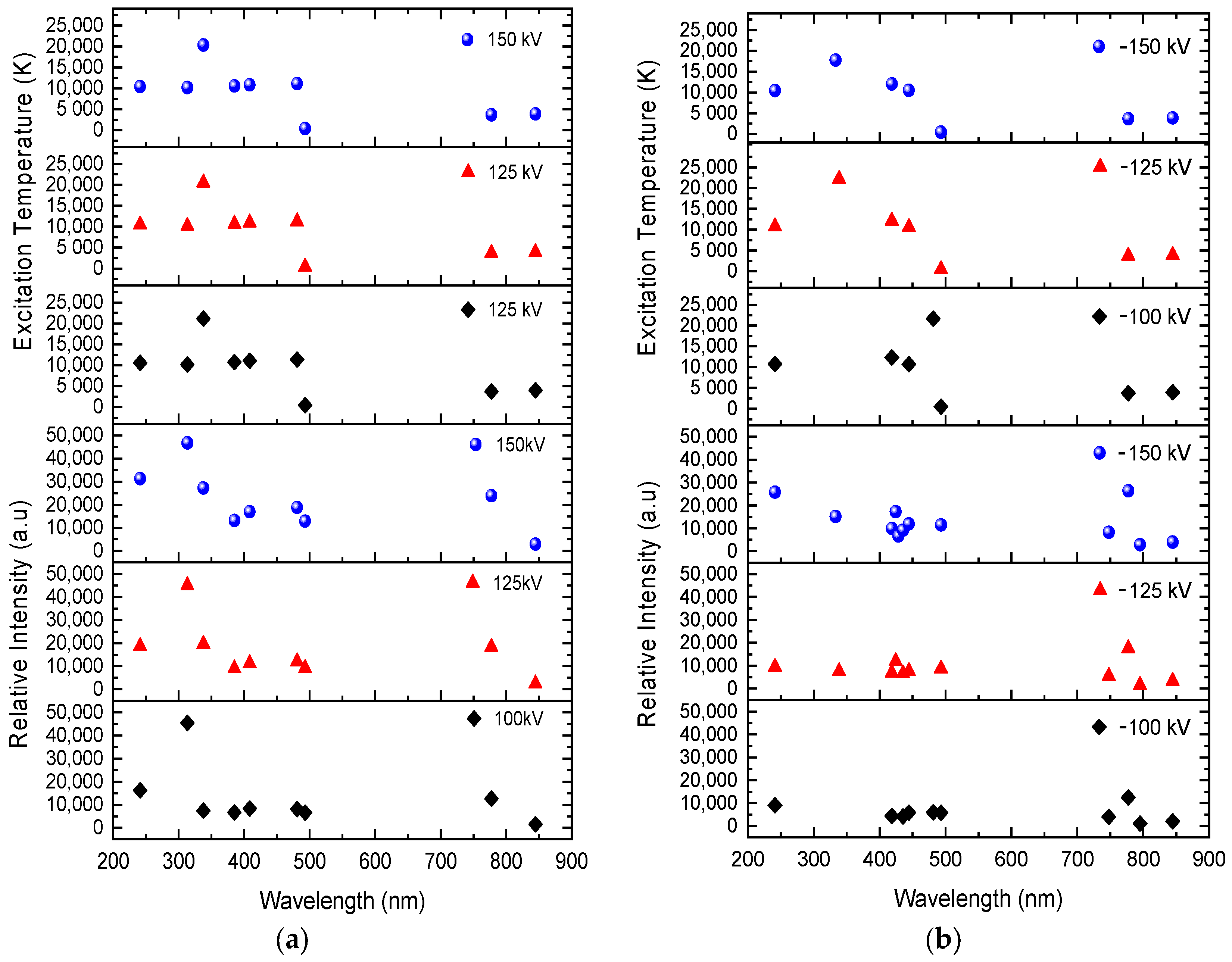
Excitation temperatures are more frequent in positive voltage rather than negative, as illustrated in Figure 7. Above 20,000 K, in both positive and negative voltages, the higher excitation temperature is found in a higher excited state of O IV. In contrast, the intensity of the positive findings occurs at temperatures between 10,000 and 22,000 K in excited state. Consequently, this allows channels to be kept easier to release Joule heating so that electrons can flow through conductive channels quicker in positive voltages than in negative voltages. Most spectral lines possess higher temperatures, which suggest a more conductive channel for more electrons to flow in an unpredictable direction until their finite decay time arrives. They then release photons at specific wavelengths. In both positive and negative breakdown voltages, this occurs regularly during the recombination process at 2.710 × 10⁻⁸ s. Remarkably, at positive voltages, there are spectral lines at 241.162 nm, 313.421 nm, and 337.806 nm that are higher in the excited state than in the recombination state. O II is only observable at 100 kV at 241.162 nm and 313.421 nm. In contrast, O II can be observed at 125 kV and 150 kV at 241.162 nm, 313.421 nm, and 337.806 nm. The peak intensities rise with applied voltage strength, but as the current grows, the field decreases.
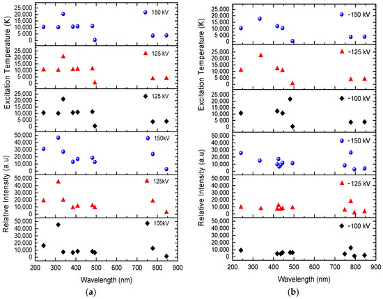
Figure 7.
Relative intensity and excitation temperature in ±100 kV, ±125 kV, and ±150 kV, based on wavelength. (a) Spectra of positive impulse voltage; (b) spectra of negative impulse voltage.
According to Equation (1), which demonstrates that intensity is proportional to electron concentrations, in quasi-neutral plasma, the electron density is nearly equal to the ion density. This implies that the electron release in the excited state is nearly equal to the electron in the recombination state. Thus, in addition to electron concentration, redundant energetic photon emission may also have contributed to the higher intensity in the excited state. When directional electrons accelerate to a breakdown in positive voltages relative to negative voltages, it is because of the coherent direction in which this emission emits photons.
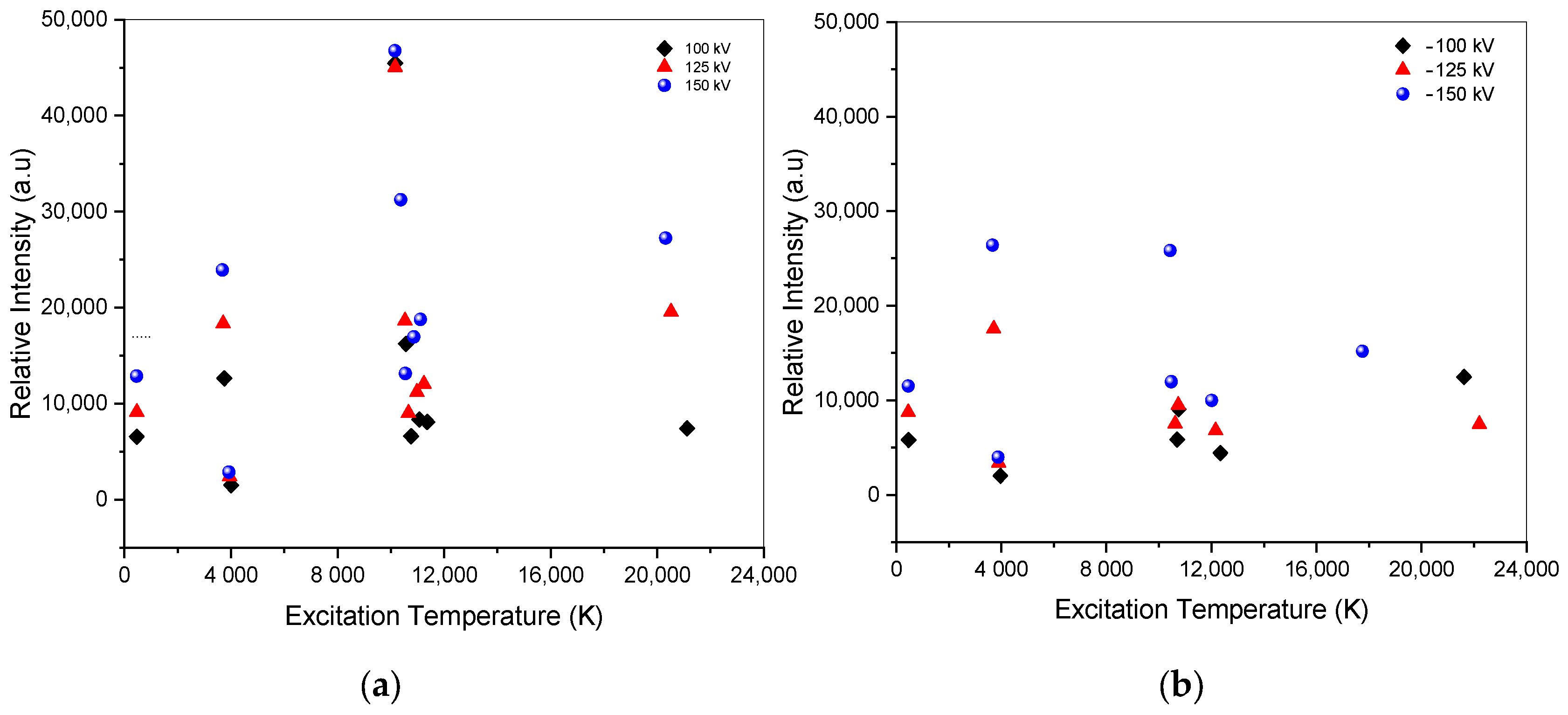
The faster decay time and the higher temperature in the excited state signify a more energetic and rapid interaction between electrons and ions to recombine in the air within the limit of the decay time. This increase leads to faster transitions of particles from excited states to lower energy states, resulting in the emission of photons at specific wavelengths. A higher excitation temperature, above 20,000 K, does not always imply a more intense and energetic initiation of photon emission, as shown in Figure 8. The excitation temperature is correlated with the excited state energy of the atom during its transition. The peak intensity is correlated with both the decay time and the electron concentration, and the higher state has a higher excitation temperature. Electron propagation increases due to coulomb collision by increasing applied voltage, contributing to strengthening electric fields in both positive and negative voltages.
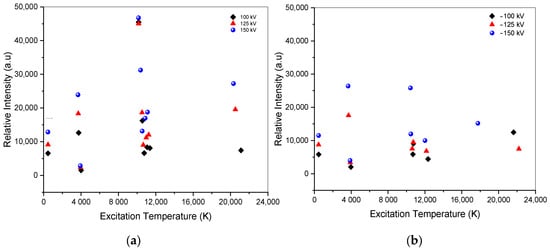
Figure 8.
Intensity vs. excitation temperature of ±100 kV, ±125 kV, and ±150 kV. (a) Spectra of positive impulse voltage; (b) spectra of negative impulse voltage.
There is another parameter that can contribute to hitting and accelerating electrons, such as the scattering process that correlates with photon emission. Therefore, the higher intensity of O II at 313.421 nm and 241.162 nm, as well as O IV at 337.806 nm, contributes to rapid breakdown time in positive voltage discharges. The higher photon emission is correlated with reference [16], which strongly emphasizes the correlation between electrons and photons for the enhancement of superconductivity and ferroelectricity in cavities, as an especially attractive possibility. Additionally, photon emission is the transition when an electron stays in the excited state for a sufficiently long time. It then spontaneously jumps to the ground state and emits light due to the electric current generated by the transition between the states, coupling the electron with photons in space and generating radiation [17]. Therefore, the coherence of the photon makes it easy to accelerate electrons in one direction, contributing to the rapid breakdown that could happen in the 10,000 s K due to photon emissions, which is indicated by the higher peak intensity in the excited state compared to the neutral state in positive voltages.
5. Conclusions
Based on our experiments with positive and negative impulse voltage discharges of ±100 kV, ±125 kV, and ±150 kV in millisecond observations, we draw the following conclusions about the rapid discharge process in positive impulse voltage:
- The higher intensities of energetic photons in the 200–400 nm bands, compared to the bands in the 400–900 nm range, are only observed in positive spectra at 241.162 nm, 313.421 nm, and 337.806 nm, with the greatest intensity observed at 313.421 nm. The distributions of oxygen atoms in the excited state are more intense in positive voltages than in negative voltages. The spectral line of O II at 313.421 nm was found to decay more quickly than other oxygen atoms in the wavelength range of 200 to 900 nm in positive voltage, falling to lower energy levels in a decay period of 1.302 × 10⁻⁸ s. Similar to this, the O II line at 418.545 nm has a decay negative voltage duration of 5.236 × 10⁻⁹ s. On the other hand, as is covered in Section 4.1, the recombination state of positive and negative voltages occurs at 2.71 × 10⁻⁸ s.
- Increased energy transitions of atomic excited states to lower energy states, which produce photons with a specific wavelength under both positive and negative voltages after their limited decay time occurs, are typically indicators of a higher temperature during the excitation process. As discussed in Section 4.2, the excitation temperatures of positive and negative voltages are different: positive voltages exceed 10,000 K in 1.302 × 10⁻⁸ s and negative voltages above 12,000 K in 5.236 × 10⁻⁹ s, respectively. Due to this, negative voltages breakdown more quickly than positive ones, requiring more heat to keep the channel stable and is not achieved until the recombination state happens in 2.710 × 10⁻⁸ s.
- Section 4.3 concludes that, for positive voltages, peak intensities are higher in the excited state than in the recombination state; however, for negative voltages, there are no higher peak intensities in comparison to the recombination state. Positive voltages tend to favor excitation temperatures between 10,000 and 22,000 K more than negative voltages in the excited state. In order to make conductive channels more practical for releasing Joule heating and allowing electrons to flow more readily in positives than in negatives, this helps maintain channels. Interestingly, at positive voltages, there are spectral lines at 241.162 nm, 313.421 nm, and 337.806 nm that are higher in the excited state than in the recombination state. These lines can help hit and accelerate electrons through processes like scattering, which is correlated with photon emission and leads to a rapid breakdown time in positive discharge.
- Positive voltages experience higher excitation temperatures than negative voltages, suggesting a more intense release of Joule heating and facilitating easier electron flows, resulting in a rapid breakdown time with higher peak intensity of O II at 313.421 and 241.162 nm, as well as OIV at 337.806 nm, than O I at 777.417 nm. Moreover, fast arc discharge is caused by these energetic photon emissions hitting and accelerating electrons.
Author Contributions
All authors made valuable contributions to this paper. Conceptualization; methodology; validation; formal analysis; investigation; writing; writing—review and editing. All authors have read and agreed to the published version of the manuscript.
Funding
This research received no external funding.
Data Availability Statement
Data are contained within the article.
Acknowledgments
This work was partly supported and sponsored by ADB AKSI Malikussaleh Univeristy. Senku Tanaka, Kindai University, was helpful in setting up devices and contributing to discussions. We also extend thanks to all members of the Remote Sensing Laboratory at Kindai University for their technical assistance.
Conflicts of Interest
The authors declare no conflicts of interest.
References
- Kojima, H.; Hotta, K.; Kitamura, T.; Hayakawa, N.; Otake, A.; Kobayashi, K.; Kato, T.; Rokunohe, T.; Okubo, H. Classification of impulse breakdown mechanisms under non-uniform electric field in air. IEEE Trans. Dielectr. Electr. Insul. 2016, 23, 194–201. [Google Scholar] [CrossRef]
- Sigmond, R.S. The residual streamer channel: Return strokes and secondary streamers. J. Appl. Phys. 1984, 56, 1355–1370. [Google Scholar] [CrossRef]
- Kip, A.F. Positive-Point-to-Plane Discharge in Air at Atmospheric Pressure. Phys. Rev. 1938, 54, 139–146. [Google Scholar] [CrossRef]
- Ducasse, O.; Eichwald, O.; Merbahi, N.; Dubois, D.; Yousfi, M. Numerical simulation and comparison with experiment for a positive point to plane corona discharges in dry air. In Proceedings of the ICPIG 2007: XXVIII International Conference on Phenomena in Ionized Gases, Prague, Czech Republic, 15–20 July 2007. [Google Scholar]
- Naidis, G.V. Dynamics of streamer breakdown of short non uniform air gaps. J. Phys. D 2005, 38, 3889–3893. [Google Scholar] [CrossRef]
- Marode, E. The mechanism of spark breakdown in air at atmospheric pressure between a positive point and plane. II. Theoretical: Computer simulation of the streamer track. J. Appl. Phys. 1975, 46, 2016–2020. [Google Scholar] [CrossRef]
- Chowdhuri, P.; Mishra, A.K.; Martin, P.M.; McConnell, B.W. The effects of nonstandard lightning voltage waveshapes on the impulse strength of short air gaps. IEEE Trans. Power Deliv. 1994, 9, 1991–1999. [Google Scholar] [CrossRef]
- David, Z.P.; Deanna, A.L.; Christophe, O.L. Transitions between corona, glow, and spark regimes of nanosecond repetitively pulsed discharges in air at atmospheric pressure. J. Appl. Phys. 2010, 107, 093303. [Google Scholar]
- Schubert, U.; Shirvani, A.; Schmidt, U. Description of the Discharge Process in Long Air Gaps under Lightning Impulse Voltage. IEEE Trans. Power Deliv. 2023, 38, 2454–2463. [Google Scholar] [CrossRef]
- Gallimberti, I.; Bacchiega, G.; Anne, B.C.; Philippe, L. Fundamental processes in long air gap discharges. Comptes Rendus Phys. 2002, 3, 1335–1359. [Google Scholar] [CrossRef]
- NIST Atomic Spectra Spectra Database Lines Form. Available online: https://physics.nist.gov/PhysRefData/ASD/lines_form.html (accessed on 23 August 2023).
- Hansjoachim, B. Pulsed Power Systems Principles and Applications; Springer: Berlin/Heidelberg, Germany; New York, NY, USA, 2006; pp. 17–18. [Google Scholar]
- Janet, L.; Pralhad, R. Foundations of Pulsed Power Technology; John Wiley & Sons, Inc.: Hoboken, NJ, USA, 2017; pp. 158–162. [Google Scholar]
- Prueitt, M. The excitation temperature of lightning. J. Geophys. Res. 1963, 68, 803–811. [Google Scholar] [CrossRef]
- Sahin, N.; Tanish, M. Electron temperature estimation of helium plasma via line intensity ratio at atmospheric pressure. Eur. Phys. J. Plus 2020, 135, 653. [Google Scholar] [CrossRef]
- Bloch, J.; Cavalleri, A.; Galitski, V.; Hafezi, M.; Rubio, A. Strongly correlated electron–photon systems. Nature 2022, 606, 41–48. [Google Scholar] [CrossRef]
- Wang, J.S.; Peng, J.; Zhang, Z.Q.; Zhang, Y.M.; Zhu, T. Transport in electron-photon systems. Front. Phys. 2023, 18, 43602. [Google Scholar] [CrossRef]

Disclaimer/Publisher’s Note: The statements, opinions and data contained in all publications are solely those of the individual author(s) and contributor(s) and not of MDPI and/or the editor(s). MDPI and/or the editor(s) disclaim responsibility for any injury to people or property resulting from any ideas, methods, instructions or products referred to in the content. |
© 2024 by the authors. Licensee MDPI, Basel, Switzerland. This article is an open access article distributed under the terms and conditions of the Creative Commons Attribution (CC BY) license (https://creativecommons.org/licenses/by/4.0/).