Abstract
Distributed energy resources have demonstrated their potential to mitigate the limitations of large, centralized generation systems. This is achieved through the geographical distribution of generation sources that capitalize on the potential of their respective environments to satisfy local demand. In a microgrid, the control problem is inherently distributed, rendering traditional control techniques inefficient due to the impracticality of central governance. Instead, coordination among its components is essential. The challenge involves enabling these components to operate under optimal conditions, such as charging batteries with surplus solar energy or deactivating controllable loads when market prices rise. Consequently, there is a pressing need for innovative distributed strategies like emergent control. Inspired by phenomena such as the environmentally responsive behavior of ants, emergent control involves decentralized coordination schemes. This paper introduces an emergent control strategy for microgrids, grounded in the response threshold model, to establish an autonomous distributed control approach. The results, utilizing our methodology, demonstrate seamless coordination among the diverse components of a microgrid. For instance, system resilience is evident in scenarios where, upon the failure of certain components, others commence operation. Moreover, in dynamic conditions, such as varying weather and economic factors, the microgrid adeptly adapts to meet demand fluctuations. Our emergent control scheme enhances response times, performance, and on/off delay times. In various test scenarios, Integrated Absolute Error (IAE) metrics of approximately 0.01% were achieved, indicating a negligible difference between supplied and demanded energy. Furthermore, our approach prioritizes the utilization of renewable sources, increasing their usage from 59.7% to 86.1%. This shift not only reduces reliance on the public grid but also leads to significant energy cost savings.
1. Introduction
Distributed energy systems can solve the problems associated with centralized generation, such as [1]: high energy losses, hazardous waste generation, and expensive infrastructure, among others. Specifically, RES with energy storage devices can be integrated to formulate HES for a reliable power supply (saving and releasing energy at the adequate time) to overcome the limitations in the wind and solar resources since their performance characteristics depend on the environment, which reduces the reliability of the power supply and imposes additional costs for providers and/or consumers [2]. On the other hand, it is necessary to consider the effects of energy management on the consumer, especially the controllable loads, to ensure an efficient energy system [3].
An MG is a distributed energy network with diverse small energy sources that work autonomously with respect to the main network [4]. An MG is classically made up of a local generation system, an energy storage system, consumers, and a connection point to the grid. The main goal of an MG is to reach a more efficient and reliable energy supply, to provide a higher quality of energy service, and to make it safer and more sustainable. The MG control problem is a distributed control problem, which requires coordination and control mechanisms for its agents without a central authority to manage them [1].
One of the incentives of this paper is to effectively coordinate and integrate the various agents in an energy system, both on the production and consumption side, to meet energy needs, maximize the use of renewable energy, and reduce energy from the main network [5]. In this way, it is expected to minimize energy costs and the need to manage the natural uncertainty of RES, along with the limited storage capacity of batteries [6]. In this sense, optimal management of these energy resources is essential to have a balance between demand and supply.
In general, an autonomous management approach of an MG for efficient demand management must be able, among other things, to turn off controllable loads when the cost of energy is high, and charge storage devices using only renewable energy, among other things. For this, new distributed control strategies, such as those based on emergent control, are necessary.
This paper aims to make use of the RTM [7] to define a self-control mechanism, so that each component takes part in the energy exchange when the circumstances are favorable. To create an emerging control proposal that enables effective energy management, it is necessary to identify the local variables and the rules for decision-making, as well as the feedback mechanisms between them. The use of an emergent control strategy based on bio-inspired techniques that allows micro-level coordination distinguishes this paper from earlier ones in the context of MG. The advantage of using the RTM over other control methods is based on the potential for creating a distributed control strategy. Each agent is prompted to act or not by its two main variables, the stimulus and threshold. The threshold is linked to the accomplishment of the goals, and the stimulus takes context information into account. Both employ RL as a self-control mechanism to control the agent’s response, enabling autonomous coordination actions. The main contributions of our paper are:
- -
- Specification of an autonomous MG management approach and self-regulating demand and load generation through emergent control mechanisms, enabling MG self-organization.
- -
- Definition of an emergent control approach based on the RTM, applicable to both the generation and demand sides. Traditionally used for task assignment problems, this is the first application of the RTM in coordination and distributed control contexts.
- -
- Development of a scheme to balance generated and demanded power, combining load from the main network and renewable sources, and controlling controllable loads and excess energy storage.
- -
- Schematization of a methodology to apply our emergent control approach in MGs in any context. Following this methodology, an MG autonomy can be specified.
In summary, this paper’s scientific novelty lies in its autonomous MG management approach, adapting the RTM—commonly used for distributed task assignment problems—as a solution for distributed control challenges in the energy sector. Our approach ensures autonomous component coordination to meet demand based on environmental conditions.
The paper is organized as follows: Section 2 discusses related work. Section 3 outlines the theoretical framework of our proposal and the process under study. Section 4 introduces our emergent control system design based on the RTM. Section 5 details the experiments conducted, quality assessment metrics, and comparisons with other works. The paper concludes with a summary and future work directions.
2. Related Work
Shahgholian [8] provides a comprehensive literature review on the operations, applications, and control of MGs, with a particular focus on local control and coordination among its components. The author also highlights various research areas, including control strategies, optimization methods, stability, and reactive power compensation techniques. This paper notably introduces control architectures like decentralized systems and variations based on MAS.
Liu et al. [9] introduce a consensus MAS DRL algorithm where each DER is an agent. These agents learn control strategies based on local states and messages received from neighboring agents.
Zhou et al. [10] discuss distributed communication network characteristics for MGs, distributed control strategies, and communication reliability issues. However, their work lacks experimental and case study analyses. Maomao et al. [11] analyze recent classifications, architectures, technologies, and methods for coordinating residential MGs, including game theory and MAS.
Zhou et al. [12] propose an MG cluster structure with an autonomous coordination control strategy that combines normalized droop-based control with adaptive control. The MG consists of an EP, a PEU, and several small MGs. Areekkara et al. [13] utilize the MAS paradigm for its autonomy, scalability, flexibility, and adaptability in MG energy management systems. Harmouch et al. [14] describe the implementation of a decentralized MAS-EMS for controlling an MG cluster. Each MG within the cluster employs a dedicated MAS-EMS for power dispatch aimed at minimizing grid power exchange. Another dedicated EMS manages power distribution among various MGs. Kofinas et al. [15] propose a cooperative MA system for managing a standalone MG’s energy. They use a distributed, cooperative RL method in a continuous action-state space, enabling MG components to operate as independent learners while coordinating through shared state variables. Fuzzy Q-learning techniques were recommended for this purpose.
Hu et al. [11] analyze recent developments in residential MG architectures and technologies, reviewing key coordination and negotiation methods. Chouikhi et al. [16] present two EM mechanisms in the context of smart buildings. To begin with, they use negotiation and multi-leader–follower game techniques to simulate the interactions between energy suppliers and building occupants. Then, in order to reduce consumer interactions and maximize energy demand cost, they suggest a distributed game theory-based scheduling method for energy demand. In this paper, the system entities are modeled using MAS.
Xu et al. [17] define a home energy management framework based on RL, using a finite Markov decision process for hour-ahead energy consumption scheduling and an extreme learning machine for predicting electricity prices and solar generation.
Arnone et al. [18] suggest a Building Management System for controlling energy flows in smart buildings integrated with various energy networks and RES, using heuristic optimization for 24 h energy generation and consumption scheduling. Aguilar et al. [19] describe a scheduling system that automatically defines hours of utilization of the controllable load devices in a home, in such a way that the use of renewable energy is maximized. To do this, they construct an autonomous cycle of data analysis tasks made up of three tasks: a scheduling task to create appliance usage schedules, and two tasks to estimate the amount of renewable energy generated and the amount of demanded load. Garcia et al. [20] conducted a systematic literature review on emergent control systems, focusing on conceptual bases, methodologies, principles, architectures, and their application in Cyber-Physical Systems, particularly in Industry 4.0.
Du et al. [21] propose a control strategy for coordinating neighboring autonomous MGs using a smart switch, focusing on power sharing without considering internal component coordination. Chai and Peng [22] propose a decentralized coordinated power control approach for islanding MGs, combining bus voltage signals with fuzzy logic control, without inter-MG interconnections. Rahman et al. [6] design a cooperative MAS for energy sharing in MGs, using graph theory to establish communication links between controllable batteries and clients. Arwa and Folly [23] explore the use of RL algorithms for MG power management, highlighting challenges and solutions.
Zheng et al. [24] analyze the energy dispatch optimization of connected MGs, proposing a distributed predictive control model with local predictive control for each MG component. Kyriakou and Kanellos [25] propose a method for coordinated scheduling of the optimal operation of active distribution networks containing complex MGs (prosumers and electric vehicles), through a strategy of centralized control [26].
Our literature review indicates that while there are numerous studies on MG control and optimization strategies, as well as architectures and methodologies, few focus on distributed control architecture addressing DER coordination. Most employ the MAS paradigm, RL, or predictive or fuzzy control models. However, case studies are limited, lacking benchmarks for performance analysis and metrics for proposal quality evaluation. Therefore, our study makes qualitative comparisons with existing works. To our knowledge, this paper is the first to propose an autonomous management approach for MGs using emerging approaches with the RTM. MAS-based control schemes allow for MG adaptation, but our emergent control approach uniquely adjusts component roles based on contextual uncertainty.
3. Theoretical Framework
The RTM used in this paper is presented in this section, as well as the MG components that will be analyzed.
3.1. Response Threshold Model (RTM)
Drawing inspiration from the behavior of labor division in ant colonies, the RTM [27] mimics ants’ sensitivity to external and internal stimuli, including the intensity of pheromone signals. This model allows the colony to adapt to varying environmental conditions [28], enabling ants to modify their behavior according to the needs and occurrences within the colony [29]. In general, the sensitivity to external/internal stimuli is quantified using a parameter called the response threshold (). An agent (ant) with a lower response threshold is more likely to become an active worker, while one with a higher threshold is less likely to be activated. In a conventional RTM for the division of labor [27], an agent j has the probability qj of work in a given moment according to the Equation (1):
where is the external or internal stimulus and is the ant’s sensitivity (response threshold) to perform task j at time t. The task assignment problem, which assumes that each worker i responds to a stimulus for a specific task j when the intensity of the stimulus exceeds the worker’s threshold for that stimulus, can be solved with the help of this model. Additionally, the ants change the intensity of the cumulative stimulus () in accordance with Equation (2) in order to exert control over the system through a process of individual or group learning by associating rewards with stimuli [27]:
In the conventional model, the variations in the stimulus’s intensity are caused by the way the task is carried out; here, Nact denotes the individuals who are actively engaged in the colony, N are the potential participants, α denotes the task’s efficiency, and δ denotes the stimulus’s increase in intensity per unit of time. In contrast, the response threshold is fixed from a simple reinforcement process, such that the threshold decreases when the corresponding task is performed and increases when the corresponding task is not performed. These combined reinforcement processes [30] allow the appearance of specialized workers; that is, some workers are more sensitive to the stimuli with a particular task j, starting from a group of initially identical individuals. The response threshold incorporating RL is expressed as follows [7]:
where yij is the proportion of entities of type i performing task j, and β and are the learning and forgetting rates, respectively. This means that according to Equation (3), in the next ∆t time units, yij fraction of entities of type I do task j, and (1 − yij) fraction of entities do nothing or something else. In this way, the RTM refers to the potential for responding to stimuli connected to tasks to address the issue of labor division in a colony.
3.2. System Modeling
An MG is a distributed electrical network with various small energy sources running parallel to the main grid [4]. The aim of an MG is to provide a higher quality of energy service, catering to the growing demand for reliable, safe, sustainable, and efficient electricity supply. Our focus is on an MG composed of a PV system, an energy storage system, an external source (the main grid), and controllable loads. Below, we describe each component’s model.
3.2.1. Photovoltaic System
A PV system generates voltage and current from solar cells arranged in series and parallel. Solar radiation affects the PV () array’s maximum power output in a variety of ways. Therefore, a control strategy is needed to efficiently utilize solar radiation to produce the most power. The output power is defined in the work of Antonanzas–Torres et al. [31] as:
where is the conversion efficiency of the PV array, S is the area of the PV array (m2), is the solar radiation (kw/m2), and is the ambient temperature [°C].
3.2.2. Energy Storage System (ESS)
One of the most popular tools to conserve electrical energy in various applications is the battery, but in addition, supercapacitors can be used to store electricity. In PV or wind energy conversion systems, batteries act as a backup. In addition to storing excess solar or wind energy during sunny or windy days, they are used to release the energy during stationary periods or at night. Various models have been put forth in the area of battery modeling. The modified simple battery model 3 is employed for this paper, but it is based on the power [W] rather than the voltage [V] [32].
where Vt is the battery’s terminal voltage, Voc is the voltage in the circuit without a load, Rint is the internal resistance of the battery, K is a polarization constant, I is the effective value of the discharge current, and SOC is the battery’s state of charge at time t (in percent).
3.2.3. Controllable Loads
Controllable loads refer to devices with manageable energy consumption. They are categorized as follows [33]:
- Type I: this type consists of various residential loads, like refrigerators, air conditioners, water heating, etc. These loads can be interrupted or controlled (e.g., for reducing demand).
- Type II: this type contains battery storage, Vehicle-to-Grid, etc., and it can be charged from or discharged to the grid (it can inject power into the grid). Furthermore, this type of load can be controlled to accommodate its grid needs.
- Type III: this type includes the rest of the appliances schedulable, which can be deferred for a suitable moment. There are diverse appliances (phone chargers, microwaves, washing machines, tumble dryers, dishwashers, vacuum cleaners, etc.).
Our research primarily focuses on controlling the energy demand of Type III controllable load appliances.
4. Design of an Emergent Control System Based on the Response Threshold Model
This section describes the components of the MG considered in this study, and our emerging control approach based on the RTM.
4.1. Distributed Control Architecture of a Microgrid
The MG analyzed in this paper, depicted in Figure 1, is designed to meet the energy demands of a residential building. Surplus self-generated energy is stored in a battery, and the power balance in the MG is maintained as per the energy conservation principle, expressed by Equation (6):
where is the total potential delivered or supplied, is the total energy consumption of the building, made up mainly of non-controllable loads (LNC) and controllable loads (LC), and is the error in the supply–demand.
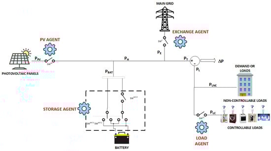
Figure 1.
Distributed control architecture for an MG.
Figure 1 introduces four agents: the PV agent denotes the control mechanism to deactivate or activate solar energy; the exchange agent manages energy supply from non-renewable sources; the storage agent handles battery charging and discharging according to specific conditions; and the load agent deactivates controllable loads when there is no renewable energy (from solar energy or battery), or the demand is greater than the power of renewable energy delivered to the energy network, and the energy market cost exceeds the price that consumers are willing to pay.
Thus, the energy system (ES) includes a PV panel, a battery, a load demand side, and a connection to the main grid. The batteries store energy during surplus generation and release it during peak load demand. The main grid is taken as a standby producer that begins to compensate when there is a deficit for the demanded energy; that is, when the storage and/or renewable generation systems fail in the supply of demanded energy. Our hybrid system’s overall power output () is indicated as follows (Equation (7)):
where is the produced power by the renewable systems (e.g., wind turbines, PV panels (), etc.) and the power in the energy storage system () (see Equation (8)), and is the main grid power.
As well, the demand will be divided into controllable () and non-controllable () (see Equation (9)):
4.2. Specification of the MAS
Utilizing the MultiAgent Systems for INtegrated Automation (MASINA) methodology [34,35], we design the emergent control approach based on the RTM. MASINA requires two steps: (i) specifying the general architecture of the system to derive the MAS, and (ii) designing each agent.
The first step involves representing the distributed system as a MAS, identifying agents, relevant variables, parameters, and behaviors, among other aspects. Table 1 summarizes the agent characterization for the MG in Figure 1.

Table 1.
Characterization of the agents.
Now it is necessary to identify the system variables which have the most influence on the agents’ behavior, in our case:
- Solar radiation.
- Demand.
- Weather conditions.
- SOC.
- Energy costs.
The second step involves designing agents based on their behavioral models using the RTM (see Figure 2). With the RTM variables (probability, stimulus and response threshold) and the internal and external variables of each agent, it is established when an agent can be active (its ON/OFF states).
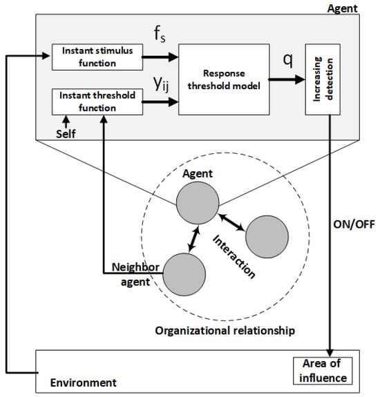
Figure 2.
RTM-based agent architecture.
Figure 2 illustrates the RTM model instantiated in each agent of our MAS. The stimulus of each agent (Equation (10)) is characterized by a cumulative function, in which is the instantaneous stimulus based on the behaviors defined in Table 1 and is the attenuation factor of the instantaneous stimulus function.
In turn, the expression of the RTM response threshold (Equation (3)), which is related to the sensitivity to the stimulus, represents the current needs in the denominator, and, in the numerator, the contribution of the agent to satisfy it. In the context of our MAS, it is specific to the role that each agent has, so it must consider aspects such as the requested demand and energy generation capacity, among other things. The following section explains these aspects in detail for each agent. Finally, the activation probability of an agent (Equation (1)) can be directly used by our agents to define their states.
In summary, the initial step in designing an emergent control system based on the RTM involves identifying the agents to define the MAS. This process includes determining their local and external variables. Once the agents are identified, we then proceed to model their behavior. This involves defining the stimulus and response threshold for each agent, dictating whether an agent will act or not. The stimulus is designed to assess context information, while the response threshold is aligned with the objectives. These components facilitate the implementation of an emergent control approach using the RTM, enabling autonomous energy management.
Equations (1), (3) and (10) are crucial for determining the behavior of each agent. They incorporate an implicit RL process as a self-control mechanism to regulate the agent’s response, along with a feedback process for sharing experiences and information. This allows for autonomous actions by the agents (see the macro-algorithm of each agent in Algorithm 1).
| Algorithm 1. Behavior of each agent based on the RTM. |
| Input: local/external variables |
Procedure:
|
| Output: state of the agent (OFF/ON) |
4.3. Emergent Control System for a Microgrid
In this section, a control model for each agent is designed based on the RTM, identifying contextual variables and components to formulate mathematical expressions of stimuli and thresholds, whose integration will form the final control system.
4.3.1. Photovoltaic Agent
Each PV agent will be activated when the stimulus increases, which occurs when energy can be produced due to weather conditions (there is radiation (), see Equation (4)), and there is demand () or capability to store energy (). In addition, it will be prone to not activate when its response threshold rises, i.e., when the power delivered to the electrical network is being covered by the PV ( > 0 and ); causing the controller to turn off. Thus, the RTM for one PV agent, in an emergent control scheme, is as follows, where is its probability to generate solar energy:
where is the maximum power output of the PV agent that varies according to solar radiation (see Equation (4)) and is an attenuation factor to make the differences of the perceived signals less sensitive.
4.3.2. Energy Storage Agent
This section presents the RTM used with the energy storage agent. This emergent control system must manage three states: consumer, producer, or passive. The following are the equations for this emergent control system:
Producer:
Equation (14) defines that the stimulus for the production is when there are demand needs (PL) that are not covered by PPV and there is stored energy (SOC). Thus, the threshold (Equation (15)) is minimized when the power supplied by the solar panels does not contribute to meeting the demand and there is also stored energy ().
Consumer:
Equation (17) defines that the stimulus happens when the battery is discharged (1 − Soc) and there is excess energy from the solar panels. The threshold (Equation (18)) is adjusted to active the agent when there is storage availability and the solar panels cover the energy needs and there is an excess ().
Passive:
Thus, is the probability of supplying energy and is the probability of consuming energy. Finally, state 3 is a passive state (see Equation (20)).
4.3.3. Main Grid Agent
The RTM applied for the exchange agent is defined in Equations (21)–(23). The agent is stimulated when the demand () is greater than the power produced by the renewable systems in the energy storage systems (); see Equation (21). The threshold is adjusted to activate the agent when the ratio between the available power and demand is not sufficient ; see Equation (22). Lastly, is the probability of activating, or not, the exchange agent:
4.3.4. Load Agent
This part of the study focuses on the RTM for the load agent, representing the controllable type III loads of customers. The load agent enables consumers to connect to the distribution network based on their needs, scheduling the use of controllable loads to utilize renewable energy or during periods of low energy prices. We assume that the uncontrollable and controllable loads of other types such as security systems, external lighting, refrigerators, and heating, are already covered.
Specifically, controllable loads of type III can be switched off when the price of electricity is high or there is no renewable energy or in the battery, among other reasons. In particular, in our context, the stimulus to turn on the controllable loads is when the energy comes from renewable sources () or when the minimum acceptable price of the energy () is not exceeded (. can be defined by the user or can be defined as the minimum or average cost of the previous day’s invoice, or something similar. The threshold is adjusted to activate the agent when there is surplus energy that comes from renewable sources ( > 1) or the price to pay for energy is interesting (). When is exceeded and there is no surplus energy, then this agent must be turned off to avoid overpayments. Finally, is the probability of activating, or not, one of the load agents (controllable loads of type III).
Table 2 summarizes the different stimulus and response threshold expressions for each agent of our MAS to model the behavior of each MG component. This allows an autonomous distributed coordination using our RTM-based emergent control approach.
Table 2.
Stimulus and response threshold expressions of each agent.
5. Experiments
This section presents the experimental protocol and scenarios for analyzing the behavior of our emergent control system based on the RTM.
5.1. Experimental Protocol
To validate the proposed controller described in Section 4, we explore a series of case studies, each with its unique characteristics. The experiments simulate a range of operational situations that controllers might encounter, such as variations in renewable generation dynamics due to weather conditions, fluctuations in uncontrolled loads, battery charging and discharging processes, and compensation from the main grid in case of deficiencies in other MG supply components. Power units are expressed in Watts [W]. We use the following performance criteria [36] to evaluate the quality of the results:
- Integral square error (ISE): This metric penalizes errors with higher values more severely than those with lower values. It is particularly useful for indicating overshoots and aggressive control, which are common following a disturbance.
- Integral Absolute Error (IAE): Unlike ISE, IAE does not differentiate between positive and negative errors. It is frequently used for online controller tuning and is suitable for typical operations and non-monotonic step responses.
We also define an objective function J for hyperparameter optimization of our models, which was defined by Equation (30), which reaches an error close to zero. Mostly, it was used for the search grid algorithm [37,38] to alter the parameters of our model.
These metrics help compare different case studies in the absence of similar works, demonstrating the feasibility and potential of our proposal. Real scenarios are modeled to conduct proof-of-concept tests. The baseline for our paper is maintaining energy balance (Equation (6)), with on/off delay time inferred through the ISE and IAE metrics. Hyperparameter optimization is an ongoing process, evolving as new agents are incorporated into the ecosystem.
5.2. Energy Scenarios
In order to demonstrate the adaptability and effectiveness of our emergent control strategy, we conducted several case studies, each designed to test the system under different conditions. Following is an overview of each one:
5.2.1. Case Study 1: Solar Energy in Remote Rural Locations
This case study analyzes the calibration and performance of the PV agent in an environment without an ESS. Conducted over 10 sunny days (measured in hours) with a constant demand of 250 W, the study aims to understand the model’s dynamics by examining the interplay between the stimulus variable and the threshold. The calibration process involved is as follows:
- Setting to modulate the instantaneous stimulus signal such that it allows variations of the accumulated stimulus in the order of tenths, to prevent overflow.
- Estimating preliminary values for and with simulations indicating the temporal trends of the stimulus and the threshold as shown in Figure 3B, with the dotted gray line representing the orientation of the signals. The adjustment is made using Equation (30) as the objective function.
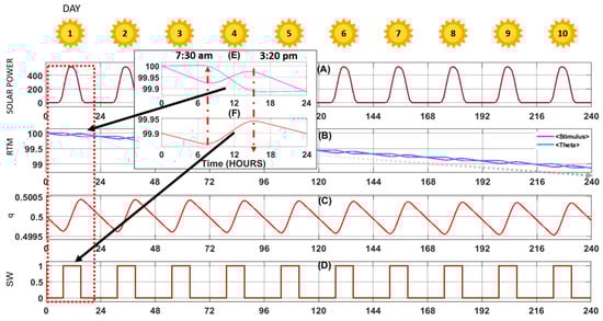 Figure 3. Solar energy in remote rural locations. From top to bottom: (A) Solar power. (B) Relationship between stimulus and threshold. (C) Probability of activation of the solar panels. (D) Smart switch activation. Figures (E,F) are the detailed and bounded views in a period of 24 h.
 - The space around the previously obtained initial values of and is explored. For that, a sweep is made of between 1 × 10⁻⁵/100 × 10−5 and between 1 × 10⁻⁵/10 × 10−5, obtaining the following values: = 2.1 × 10⁻⁴ and = 1 × 10⁻⁵ and a = 0.0641.
The PV agent is activated in response to solar radiation (see Equation (4)) and consumer demand as there are no ESSs to store the produced energy. Figure 3 exhibits the key variables involved in the PV agent, with stable sunny days (as shown at the top of Figure 3).
Figure 3A depicts the consistent solar power available throughout the study, providing a foundational context for the PV agent’s operation. This consistent availability of solar radiation is crucial for the agent’s activation. In addition, it is observed how the interaction between the stimulus variables (context-dependent, such as solar radiation) and threshold intertwine to exhibit a dynamic (see Figure 3B,E,F) which results in the probability of activation or deactivation of the PV agent (see Figure 3C,D) that comes into operation when conditions are favorable, which will be explained below.
Figure 3E shows a day (24 h) during which the PV agent must be used to meet the demand from sunrise to sunset. Figure 3F illustrates how the stimulus (pink line) exhibits a decreasing behavior at night and an increasing behavior with sunrise, which is expected. In addition, the threshold (blue line) decreases when the solar panels contribute to satisfying the demand, translating into an increase in probability when there is solar radiation (see Figure 3F). At approximately 7:30 am, the PV agent switch is activated to supply power to the load, and remains activated for almost 8 h, until its deactivation at 3:20 p.m. when the power generated by the panel is no longer sufficient. This reveals that the activation mechanism is based on the probability signal (stimulus due to the sun), which allows the switches to be automated.
The simulation was conducted 20 times, and the results, including the averages and worst results for the ISE and IAE metrics, are summarized in Table 3. The standard deviation (S), trending towards zero, indicates the control system’s stable performance. This pattern of stability, as reflected in the ISE and IAE results, is consistent with the results achieved in the other case studies (see Section 5.2.2, Section 5.2.3, Section 5.2.4, Section 5.2.5, Section 5.2.6, Section 5.2.7 and Section 5.2.8). This pattern of stability, as reflected in the ISE and IAE results, is consistent with the results achieved in the other case studies (see Section 5.2.2, Section 5.2.3, Section 5.2.4, Section 5.2.5, Section 5.2.6, Section 5.2.7 and Section 5.2.8).
Table 3.
Performance metrics for case study 1.
Table 3 provides a comprehensive overview of the system’s behavior by presenting a set of metrics. In the worst-case scenario, where the power supply–demand discrepancy (∆P) is at its maximum, ISE and IAE values reach their highest. These values are compared to the average ISE (1.01 × 10⁷) and IAE (4.03 × 10⁴) recorded during the experiment. The difference in magnitude between the worst-case and average scenarios is approximately 67.47% for ISE and 67.17% for IAE. This implies that over the 10-day (or 240-h) study period, the agent remained deactivated 67% of the time, translating to the PV agent being active for about 33% of the time. In terms of power supply, this equates to approximately 79 h or 3.3 days of activation. Table 4 details the parameters derived from the hyperparameter optimization process specific to this case study.
Table 4.
Optimization of hyperparameters for functional control mode.
The most relevant parameters of our model are the initial values of the stimuli and thresholds, as well as the factors used by each model, which significantly impact the speed and effectiveness of the reinforcement process. Notably, for each parameter, the forgetting factor outweighs the learning factor. This characteristic enables the agents to effectively utilize and build upon the knowledge they have acquired. Additionally, the attenuation factor, which plays a crucial role in modulating the stimulus, is kept relatively small. This careful calibration ensures that the stimulus is adjusted in a controlled manner, contributing to the overall precision and responsiveness of the model.
5.2.2. Case Study 2: Variable Solar Power in Remote Rural Areas
In a typical scenario encountered in rural or remote areas, such as farms without electricity service, inhabitants often turn to alternatives like solar systems to harness daylight radiation. This case study, inspired by the research of Yousif et al. [39], examines renewable energy sources without ESS, focusing on the quality and stability of the power delivered. Over a 10-day period, marked by variability in weather conditions and demand, the study explores these dynamics. The findings are presented in Table 5 and Figure 4.
Table 5.
Performance metrics for case study 2.
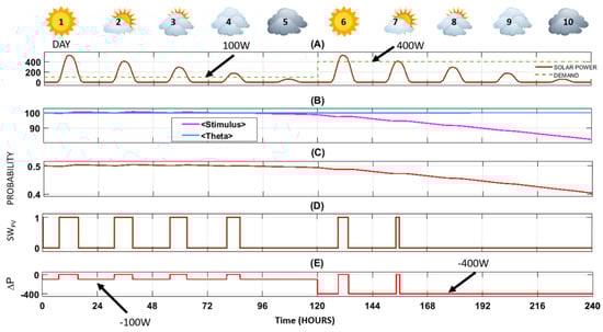
Figure 4.
Variable solar power in remote rural areas with load demand. From top to bottom: (A) Continuous line represents solar power as a function of irradiance and the dotted line represents the real demand. (B) Relationship between stimulus and threshold. (C) Probability of activation of the solar panels. (D) Digital control signal for activation/deactivation of the switch by the PV agent. (E) Difference between the power delivered and consumed.
In Figure 4A, there are two significant shifts in energy demand. For the initial five days, the demand remains low at 100 W, allowing for optimal use of the available solar power. However, from day 6 onwards, the demand surges to 400 W. Consequently, solar energy is only sufficient to meet this increased demand on days 6 and 7. Starting from day 8, the solar radiation drops to levels too low to activate the Photovoltaic (PV) agent, as illustrated in Figure 4D.
Figure 4E highlights the energy deficit resulting from the lack of alternative energy sources to fulfill the demand. This deficit is corroborated by the data in Table 5, where is close to the worst of the scenarios, with 93.33% for ISE and 82.6% for IAE, which means the percentage that fails to satisfy the demand. As a result, the PV agent’s contribution is limited to 17.4%, with the shortfall leading to a blackout.
These outcomes, derived from 20 simulations as shown in Table 5, also reveal a standard deviation (S) tending towards zero. This indicates that despite the challenging conditions and the resultant shortfall in energy supply, the control system’s performance remains stable.
5.2.3. Case Study 3: Coordination between Energy Supply Agents
The objective of this case is to evaluate the coordination of the energy supply agents (solar energy and main grid) over a 10-day period characterized by variable sunny conditions. This scenario, typical of a residential setting, assumes a constant demand of 250 W with unvarying costs. The study, inspired by the findings in the work of Hu et al. [11], aims to assess how photovoltaic systems and the main electrical network collaborate to meet the energy needs of residential consumers.
In this case study, cloudiness significantly impacts the solar energy output, as observed in Figure 5A. The reduction in solar radiation due to cloud cover, particularly on days 2–5 and 7–10, leads to a decreased contribution from solar energy, which is clearly demonstrated in Figure 5B. The impact is most pronounced on days 4–5 and 9–10, where the cloudiness is so substantial that the Photovoltaic (PV) agent remains inactive, unable to generate adequate power due to insufficient radiation.
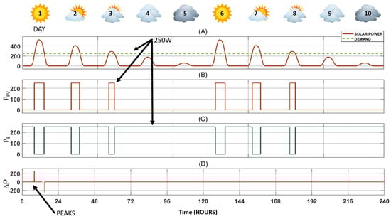
Figure 5.
Failure in the energy storage system. From top to bottom: (A) Continuous line represents solar power as a function of irradiance and the dotted line represents the real demand. (B) Real power delivered by the solar panels. (C) Power from the external electrical grid. (D) Difference between the power delivered and consumed.
During these days, with the PV agent being inactive, the residential demand for power cannot be met by solar energy alone. Consequently, as depicted in Figure 5C, the electricity demand is fulfilled by an external power source. This reliance on an external grid during periods of reduced solar output underscores the importance of having a diversified energy supply, particularly in residential settings where consistent power availability is crucial.
Figure 5D illustrates the disparity between the energy supplied and the energy consumed. This difference is quantitatively depicted in Table 6, which shows exceptional demand satisfaction (∆P = 0), marked by a singular peak in both the IAE and ISE, each at 0.01%. The distribution of contributions from various components of the energy ecosystem is as follows: solar panels account for 13.13%, the battery contributes 0.0%, and the external power supply provides the majority at 86.88%. This distribution underscores the predominant role of the external power supply in this energy mix.
Table 6.
Performance metrics for case study 3.
5.2.4. Case Study 4: Storage System with Failures
This case study centers on examining the coordination among PV agents, the battery, and the main electrical network in a situation where the battery, initially 100% charged, experiences a deep discharge due to a malfunction in its recharging mechanism, rendering its recovery impossible. Uniformity in energy costs and demand is maintained in this typical residential scenario. However, the battery charge and discharge controller encounter an issue in its electrical system, preventing proper charging of the storage system. This study is grounded in the research presented by Hu et al. [11].
Figure 6A displays solar power alongside the constant demand, highlighting days (such as 4, 5, 9, and 10) where solar power is insufficient due to weather conditions. In addition, Figure 6B shows how the photovoltaic agent is activated when there is solar radiation, which influences the time of the power delivered by the solar panels due to the level of radiation. Also, it is observed between the period of absence of solar radiation or cloudiness (see Figure 6A) that the battery comes into operation to supply the demand of consumers (Figure 6C). On day 4, with inadequate irradiation, solar panels fail to activate, and the storage device must supply energy all day. However, a failure in the battery agent leads to its complete discharge. (Figure 6D). The exchange agent intermittently compensates until it fully assumes supply due to the battery’s complete discharge (SOC = 0) and insufficient solar radiation from day 9 onwards (Figure 6E).
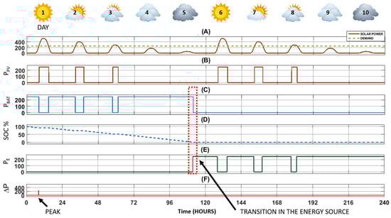
Figure 6.
Storage system charging process failure. From top to bottom: (A) Continuous line represents solar power as a function of irradiance and the dotted line represents the real demand. (B) Real power delivered by the solar panels. (C) Battery power. (D) Dotted line represents the SOC battery charge percentage. (E) Power of the external electrical grid. (F) Difference between the power delivered and consumed.
Figure 6F depicts the balance achieved in the electrical network, fulfilling demand through the joint coordination of the agents and compensating for the deficiencies due to failures. Notably, the utilization of the storage device improves the metrics compared with case study 2 by reducing peaks caused by the entry of the external electrical network. The figure shows the difference between the energy delivered and consumed, as quantitatively represented in Table 7, with excellent demand satisfaction (∆P = 0). A single peak is noted in the IAE (0.02%) and ISE (0.04%) metrics, with the latter being higher. The contributions from each component of the energy ecosystem are as follows: solar panels at 13.13%, the battery at 39.95%, and the external power supply at 46.96%. This distribution highlights the significant influence of climatic conditions on renewable energy production (solar energy) and the increased reliance on external energy sources due to the battery’s failure.
Table 7.
Performance metrics for case study 4.
5.2.5. Case Study 5: Storage System Failure and Restoration
Case Study 5 examines the ecosystem’s response to a battery failure in a typical residential setting, where the battery, initially fully charged, encounters a communication failure. This failure prevents the SOC variable from being detected by any system agent during the first five days. After 120 h, the communication issue is resolved. The scenario assumes variable solar radiation due to weather conditions and a constant demand over 10 days. This study, based on the insights from Hu et al. [11], analyzes the impact of a battery agent problem and its subsequent restoration on the overall energy supply system.
Figure 7A displays solar power in relation to irradiance alongside the actual demand. It highlights days, such as 4, 5, 9, and 10, where solar power is insufficient due to weather conditions. In addition, Figure 7B illustrates the activation of the PV agent and its influence on the power delivered by the solar panels, dictated by the level of solar radiation. Figure 7C shows that for the first five days, the battery does not operate due to the failure in communicating the SOC variables. Once this issue is resolved, the battery resumes operation and supplies the required power for the subsequent days. In Figure 7D, the dotted line represents the SOC battery charge percentage throughout the period, and Figure 7E indicates the periods when the power from the external electrical grid is utilized, particularly after the battery is fully discharged on the 10th day.
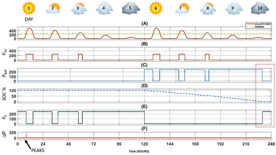
Figure 7.
Storage system failure and restoration. From top to bottom: (A) Continuous line represents solar power as a function of irradiance and the dotted line represents the real demand. (B) Real power delivered by the solar panels. (C) Period where the battery power is supplied. (D) Dotted line represents the SOC battery charge percentage. (E) Period where the power of the external electrical grid is used. (F) Difference between the power delivered and consumed.
Figure 7F reveals the difference between the energy delivered and that consumed, whose behavior is represented quantitatively through Table 8, with excellent demand satisfaction (∆P = 0), and with a single peak expressed in the metric IAE (0.03%) and ISE (0.09%), the latter being higher due to the presence of the peak. The contribution of each of the components of the energy ecosystem is distributed as follows: 13.13% the solar panels, 39.94% the battery, and 46.96% the external power supply, which demonstrates the high influence of climatic conditions on production from renewable sources (solar energy), and the greater participation of the external energy source.
Table 8.
Performance metrics for case study 5.
5.2.6. Case Study 6: Normal Operation of the MG with Constant Demand
The aim of this case study is to evaluate the performance of the energy storage agent in managing energy supply and consumption processes under constant demand. It operates under the assumption of stable energy costs over time ( > ), and varying solar radiation, as depicted in see Figure 8A. This scenario is typical of a residential environment powered by various sources, with the study focusing on the coordination of its components. The foundational research for this case is drawn by Zhou et al. [10].
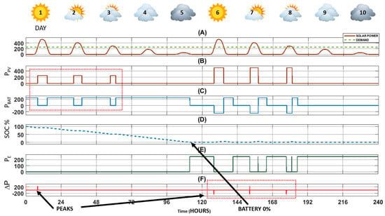
Figure 8.
Normal operation of the MG with constant demand. From top to bottom: (A) Continuous line represents solar power as a function of irradiance and the dotted line represents the real demand. (B) Real power delivered by the solar panels. (C) Period where the battery power is supplied. (D) Dotted line represents the SOC battery charge percentage. (E) Period where the power of the external electrical grid is used. (F) Difference between the power delivered and consumed.
Figure 8A shows the solar power with constant demand, evidencing that there are days where the solar power is not enough to satisfy the demand, such as days 4, 5, 9, and 10, due to weather conditions. In addition, Figure 8B shows how the PV agent is activated according to the solar radiation and load demand. On the one hand, it is evident that in the absence of solar energy, the storage device starts to work and is activated again when the power of the panel is not enough, which is highlighted between days 1 and 3 of Figure 8B,C. On the other hand, the battery is completely discharged on day 5, and tries to recover slowly, but, motivated by the demand and variability of the climatic conditions, the SOC tends to zero (see Figure 8D). Thus, the external power system comes into operation intermittently from day 5, and becomes permanent from day 9, due to insufficient solar radiation and battery discharge.
Figure 8F presents the difference between the energy delivered and consumed. This behavior, quantitatively depicted in Table 9, shows excellent demand satisfaction (∆P = 0), with occasional peaks in the IAE (0.09%) and ISE (0.16%) metrics, the latter being higher due to the quantity and magnitude of the peaks. Meanwhile, the IAE remains lower than the ISE due to the infrequent occurrence of these peaks. The energy contributions are distributed as follows: solar panels at 13.11%, the battery at 46.58%, and the external power supply at 40.31%. This distribution highlights the significant impact of climatic conditions on renewable energy production (solar energy) and the subsequent effects on the battery charging processes.
Table 9.
Performance metrics for case study 6.
5.2.7. Case Study 7: Normal Operation of the MG with Variable Consumption
The focus of this case study is to analyze the coordination between the components of an MG—specifically the solar panels and external power source—in a scenario where there is variable consumption against a backdrop of constant solar radiation over a 10-day period. The battery in this scenario is fully functional and charged (charge and discharge). This residential scenario, drawing on various energy sources, examines the coordination between the MG components in response to demand variations. The study is based on the research conducted by Zhou et al. [10].
Figure 9A shows the solar power and the variation in the demand of the electrical network, highlighting the excess energy that will allow the battery to be charged. The power generated by PPV (solar panels) is used depending on the demand needs and availability of storage in the battery (SOC << 1). For example, on days 1 and 2, only what is required by the load is supplied, while for the rest of the days, both the demand and the battery charge are covered (see Figure 9B). It can also be seen in Figure 9C,D, the power delivered by the battery and the percentage (SOC), respectively, where it is fully discharged on day 6 and begins a gradual recovery process, due to the demand decreases at the end of day 7. Between days 6 and 8, the battery is completely discharged, so the external power source comes into operation (see Figure 9E).
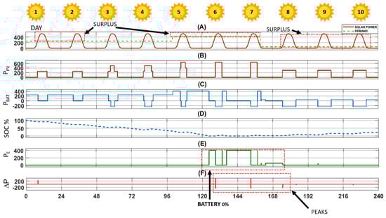
Figure 9.
Normal operation of the MG with variable consumption. From top to bottom: (A) Continuous line represents solar power as a function of irradiance and the dotted line represents the real demand. (B) Real power delivered by the solar panels. (C) Period where the battery power is supplied. (D) Dotted line represents the SOC battery charge percentage. (E) Period where the power of the external electrical grid is used. (F) Difference between the power delivered and consumed.
Figure 9F presents the difference between the energy delivered and consumed. This behavior, as quantified in Table 10, indicates excellent demand satisfaction (∆P = 0), with occasional peaks expressed in the metrics IAE (0.73%) and ISE (0.19%). The ISE is lower due to the frequency and magnitude of the peaks, whereas the IAE is higher, reflecting an increase in magnitude due to demand variations on days 6 and 7. The energy contributions are distributed as follows: solar panels at 27.92%, the battery at 58.38%, and the external power source at 13.72%. This distribution signifies that 86.26% of the energy comes from renewable sources, underscoring the MG’s effective management and utilization of renewable energy.
Table 10.
Performance metrics for case study 7.
5.2.8. Case Study 8: Energy Price Variability
This case study investigates the functionality of the entire energy ecosystem amidst energy price fluctuations over a 10-day period, focusing on how these changes affect behavior around the cost of comfort. The scenario assumes constant solar radiation, a fully charged (100%) battery at the start, and normal operation for charging and discharging processes. The non-controllable loads consume 200 W, and the controllable loads consume 50 W, representing a scenario with diverse energy sources and fluctuating energy costs.
The dotted line in Figure 10A indicates solar power related to irradiance, while the solid line shows the actual potential delivered by the solar panels. For the initial two days, the energy supply is solely from the battery and solar agents, as shown in Figure 10B. Despite high battery charge levels and solar panel energy surpluses, these surpluses are not utilized until the third day.
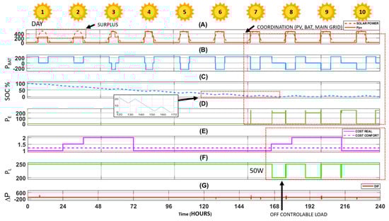
Figure 10.
Energy price variability. From top to bottom: (A) The dotted line represents solar power as a function of irradiance and the solid line represents the real potential delivered by the solar panels. (B) Continuous line is the battery power supplied. (C) Dotted line represents the SOC battery charge percentage. (D) Period where the power of the external electrical grid is used. (E) The dotted line represents the cost of comfort and the continuous line the variations in the price of energy. (F) Demand or power consumed by the apartment. (G) Difference between the power delivered and consumed.
The battery has a high percentage of load, and the energy surpluses of the solar panels are not used, but from the third day on, the excess energy from the solar panels is gradually used to charge the battery, which is evidenced by the overlapping of both signals (see Figure 10A) This charge is very tenuous (See Figure 10C). Figure 10B shows the three states of the battery: when PBAT > 0 then it supplies power; when PBAT = 0 then it does nothing; and when PBAT < 0 then it charges. On day 7th, the batteries are completely discharged for the first time, and that is when the external electrical energy comes into operation to supply the energy deficiencies (see Figure 10D). It should be noted that the batteries manage to partially charge themselves in periods of excess solar energy, but are not enough to achieve 100% charge. So, coordinated control is obtained between the solar panels, the batteries and the external electrical network.
Figure 10E shows the variations in the price of energy. When the batteries are charged in the first 6 days, despite the cost increase, it is not relevant because the external source does not act. But then, in the second cycle of variations in the price of energy that occurs between days 8 and 9, it affects the operation of the electrical network, which causes the deactivation of controllable loads to reduce consumption. Most of the time (91.46%), full energy supply is guaranteed to both controllable and non-controllable loads, but only 8.54% of the time, controllable loads are turned off due to high energy prices.
Figure 10G quantitatively represents the difference between the energy delivered and consumed. In other words, a measure of satisfaction of consumers who seek to have the trend as close to zero as possible, which is shown in Table 11, when the peaks and transitions of the energy sources are minimal with values of 0.10% in the case of the IAE and 0.17% in the ISE. The latter is higher because it penalizes the peaks that appear. To calculate the above measurements, the worst case is considered when the error is maximum (250 W) during the 10 days.
Table 11.
Performance metrics for case study 8.
5.3. General Discussion
The results of the case studies, reflecting the contributions of the MG generation sources, are summarized in Table 12. The data are expressed in hours, days, and percentages relative to a period of 240 h/10 days/100 percent. Each case study explores a variety of scenarios that can occur in electrical networks. These scenarios include weather variations, component failures, market price fluctuations, and changes in consumer demand, among others.
Table 12.
Summary of the case studies.
Figure 11 graphically represents the percentage contribution of each component. In cases 1 and 2, only the solar panels are involved, with differences between the two cases due to climatic variability.
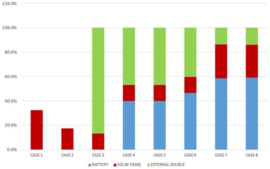
Figure 11.
Contribution of supply sources in each case study.
According to Figure 11, blackouts are caused by an energy deficit when other supply sources are absent, leading to a vulnerable and deficient electricity supply. Conversely, from cases 3 to 8, there is evident perfect coordination among the various agents to ensure energy supply under any condition. Cases 4–6 exhibit similar behaviors, as do cases 7 and 8, where most of the energy supply is from renewable sources. This situation is advantageous for consumers, as renewable energy is generally cheaper and less polluting than fossil fuel-based sources such as gas and oil.
This paper has demonstrated the technical feasibility of our proposal through simulations. However, for real-world implementation, other technological aspects must be considered. Specifically, the emerging agent-oriented RTM-based controller would operate at the tertiary level of an MG control architecture, necessitating coordination, control, and communication processes with higher-level agents. This would require communication capabilities depending on the distributed nature of the MG components. For wireless communication needs, technologies like GSM, GPRS, 3G, 4G, and Wi-Max could be utilized; ZigBee, WiFi, or Bluetooth are suitable for shorter distances. Wired solutions might include Power Line Communication (PLC), fiber optics, and DSL for longer distances, or RS485 and Ethernet for shorter distances [9].
5.4. Qualitative Comparison with Previous Works
In comparing our work with previous studies (refer to Table 13), several criteria have been considered:
Table 13.
Comparison with previous works.
- Context of Distributed Control: one criterion is whether the study is within the context of distributed control.
- Energy Problem Involving Both Supply and Demand: another criterion is whether the study addresses the energy problem involving both supply and demand simultaneously.
- Consideration of New Agents: lastly, we consider if the study incorporates dynamically new agents, such as new renewable energy sources.
The x symbol on Table 13 indicates that this work meets that criterion.
Following is a qualitative comparison with some of the previous works: Harmouch et al. [14] suggest a decentralized MA-EMS with the goal of minimizing power exchange with the main grid. While it shares a similar architecture with our paper, it does not search into the coordination between different elements or variations in market prices, and the study time periods are shorter. Additionally, its objective is to minimize grid reliance rather than satisfy consumer needs.
Kofinas et al. [15] recommend a cooperative MAS for managing the energy of a stand-alone MG. The MAS learns to control the MG components, but it requires previous experience to define the control rules. Moreover, it does not consider the participation of controllable loads on the demand side. Zhou et al. [9] propose an autonomous coordination control strategy for MGs, and Areekkara et al. [13] study a MAS approach to model an MG EMS with diverse forecasting agents and a real-time correction agent.
Chouikhi, et al. [16] present electricity management mechanisms in smart buildings to reduce total energy cost and the peak to the average consumption ratio, and maximize the exploitation of renewable energy. Unlike our proposal, which focuses on controllable loads, this work analyzes various loads within building apartments but does not detail their distribution within the building.
Zheng et al. [40] examine self-organization algorithms that are appropriate for task distribution in industrial manufacturing processes with significant task dependencies. They propose two algorithms based on the RTM for task dependencies. They only rely on local interactions between the relevant agents and the environment for decision-making. It is a different application of the RTM compared to our approach as an emergent control strategy.
The rest of the works [9,11,17,18] fall along the same lines as the previous ones: they do not simultaneously consider both sides (producer and consumer), or they do not allow distributed control or the natural integration of new agents. These aspects are covered by our proposal. It is worth highlighting the works [11,12,19] that address trends in coordination strategies around energy management systems as an MG. In these works, it can be verified that the RTM has not been previously used, showing that our RTM-based approach is an innovative proposal. Additionally, this paper indicates the way to specify an MG using the MAS paradigm with an emergent coordination approach between its agents (see Section 4.2).
6. Conclusions
Based on the emergent control paradigm, this paper proposes a distributed control architecture for MGs. Specifically, it is based on the RTM, which was inspired by how ants react to internal or external stimuli of local variables in their environment. The paper suggests an emergent control approach for MGs composed of heterogeneous agents, including batteries, solar panels, controllable loads, and external energy sources. These agents must coordinate to satisfy consumer demand.
One of the main features of our emergent control method is its robustness. It adapts to component failures, changes in climatic conditions, or economic variables, ensuring the achievement of global goals. The activation mechanisms derived from this approach significantly improve performance, with IAE metrics as low as 0.01% (in case study 3), indicating minimal difference between supplied and demanded power.
The research results demonstrate the potential of this approach to address several challenges in the energy ecosystem: (i) MG component decentralized coordination based on local environmental knowledge; (ii) Robustness in distributed control actions in the face of different failures (see cases 3, 4 and 5); (iii) RES prioritization. From cases 3 to 8, there is evidence of perfect coordination between the various agents to guarantee the energy supply in any condition ∆P = 0. Cases 4–6 show similar behaviors, as well as cases 7 and 8, where most of the energy comes from renewable energy sources, 59.7% and 86.1%, respectively. The main findings of the research work focus on the definition of an autonomous distributed control based on the RTM, and the definition of a methodology to apply our emergent approach to control an MG. Our approach allows maximizing the use of renewable energy, uses controllable charging when it is least expensive, and optimizes the use of batteries, among other things. On the other hand, one of the main limitations of this work is the implementation in a reduced number of energy agents.
Future work aims to integrate additional RES such as wind and geothermal and consider their joint performance. The study will also dig into controllable loads and other agents like electric vehicles, exploring various user comfort levels for load adjustment. The emergent control proposal will be integrated into a MAPE-K (Monitor-Analyze-Plan-Execute plus Knowledge) model [41] for smart energy management in smart grids. Furthermore, the approach will be implemented in an energy simulator like ESDL-based Energy System Simulator (ESSIM) [42] and investigated for compatibility with advanced RL models, including Deep RL.
Additionally, other conditions, such as penalties stipulated in electricity supply contracts for interruptions to consumer supply, can be incorporated into the design of our emerging controller. Under these conditions, maintaining the stability of the MG requires action on the electricity supply networks rather than on the consumers. Another aspect for future studies is the monitoring of frequency values to control the balance between the electrical energy produced and consumed. Finally, while future work will concentrate on distributed control issues, there is also a potential to explore more complex component models and apply MG design methods to size components appropriately according to various needs and operational requirements.
Author Contributions
Conceptualization, M.G. and J.A.; Methodology, J.A.; Validation, M.D.R.-M.; Formal analysis, M.G. and J.A.; Investigation, M.G., J.A. and M.D.R.-M.; Writing—original draft, M.G.; Writing—review & editing, J.A. and M.D.R.-M. All authors have read and agreed to the published version of the manuscript.
Funding
This project received funding from the European Union’s Horizon 2020 research and innovation programme under the Marie Skłodowska-Curie grant agreement No 754382 GOT ENERGY TALENT. M.D.R.-M. is supported by the JCLM project SBPLY/19/180501/000024 and the Spanish Ministry of Science and Innovation project PID2019-109891RB-I00, both under the European Regional Development Fund (FEDER).
Data Availability Statement
The data presented in this study are available on request from the corresponding author.
Conflicts of Interest
The authors declare no conflict of interest.
Disclaimer
The content of this publication does not reflect the official opinion of the European Union. Responsibility for the information and views expressed herein lies entirely with the authors.
Nomenclature and Abbreviations
| Subscripts | |
| i | For agents/individuals |
| j | For tasks, j = {PV, ESS, UG} |
| Variables | |
| Response threshold | |
| s | Stimulus |
| q | Activation probability |
| Nact | Quantity of active entities |
| N | Quantity of entities that may be active in the colony |
| Instant stimulus | |
| Portion of entities of type i doing task j | |
| Maximum active power output PV [W] | |
| Solar radiation [kw/m2] | |
| Ambient temperature [°C] | |
| Terminal voltage of the battery [V] | |
| Battery state of charge at t [%]. | |
| The effective value of the discharge current [A] | |
| Total active power generated [W] | |
| Error in the supply-demand [W] | |
| Generated active power by the renewable systems [W] | |
| Main grid active power [W] | |
| Active power in the energy storage system [W] | |
| Total energy consumption or demand [W] | |
| Power consumed by controllable loads [W] | |
| Power consumed by uncontrollable loads [W] | |
| Comfort cost | |
| Market cost | |
| Abbreviations | |
| DER | Distributed energy resources |
| DRL | Deep Reinforcement Learning |
| EP | Energy pool |
| PEU | Power exchange unit |
| EMS | Energy Management System |
| ES | Energy system |
| ESS | Energy storage system |
| HES | Hybrid energy systems |
| LC | Controllable loads |
| LNC | Non-controllable loads |
| MAS | Multiagent Systems |
| MASINA | Multiagent Systems for Integrated Automation |
| MG | Microgrid |
| PV | Photovoltaic |
| RES | Renewable Energy Systems |
| RTM | Response Threshold Model |
| RL | Reinforcement Learning |
| UG | Utility grid |
| WECS | Wind energy conversion systems |
| Parameters | |
| α | Scale factor that measures the efficiency in performing the task |
| δ | Increase in the stimulus’s intensity per unit of time |
| β | Learning rate |
| Forgetting rate | |
| Conversion efficiency of the PV array | |
| Area of the PV array [m2] | |
| Circuit voltage [V] | |
| Internal resistance of the battery [Ω] | |
| Polarization constant | |
| Attenuation factor of the instantaneous stimulus function (fs) | |
References
- Ray, P.K.; Mohanty, S.R.; Kishor, N. Small-signal analysis of autonomous hybrid distributed generation systems in presence of ultracapacitor and tie-line operation. J. Electr. Eng. 2010, 61, 205–214. [Google Scholar] [CrossRef]
- Moghaddas-Tafreshi, S.; Jafari, M.; Mohseni, S.; Kelly, S. Optimal operation of an energy hub considering the uncertainty associated with the power consumption of plug-in hybrid electric vehicles using information gap decision theory. Int. J. Electr. Power Energy Syst. 2019, 112, 92–108. [Google Scholar] [CrossRef]
- Anvari-Moghaddam, A.; Rahimi-Kian, A.; Mirian, M.S.; Guerrero, J.M. A multi-agent based energy management solution for integrated buildings and microgrid system. Appl. Energy 2017, 203, 41–56. [Google Scholar] [CrossRef]
- Ahmethodzic, L.; Music, M. Comprehensive review of trends in microgrid control. Renew. Energy Focus 2021, 38, 84–96. [Google Scholar] [CrossRef]
- Aguilar, J.; Garcès-Jimènez, A.; Gallego-Salvador, N.; de Mesa, J.G.; Gomez-Pulido, J.; Garcìa-Tejedor, À. Autonomic Management Architecture for Multi-HVAC Systems in Smart Buildings. IEEE Access 2019, 7, 123402–123415. [Google Scholar] [CrossRef]
- Rahman, M.S.; Orchi, T.; Saha, S.; Haque, M.E. Cooperative Multiagent Based Distributed Power Sharing Strategy in Low-Voltage Microgrids. IEEE Trans. Ind. Appl. 2020, 56, 3285–3296. [Google Scholar]
- Bonabeau, E. Fixed Response Thresholds and the Regulation of Division of Labor in Insect Societies. Bull. Math. Biol. 1998, 60, 753–807. [Google Scholar] [CrossRef]
- Shahgholian, G. A brief review on microgrids: Operation, applications, modelling, and control. Int. Trans. Electr. Energy Syst. 2021, 31, e12885. [Google Scholar] [CrossRef]
- Liu, Z.; Xiang, T.; Wang, T.; Mu, C. Cooperative Optimization Strategy for Distributed Energy Resource System using Multi-Agent Reinforcement Learning. In Proceedings of the IEEE Symposium Series on Computational Intelligence, Orlando, FL, USA, 5–7 December 2021; pp. 1–6. [Google Scholar]
- Zhou, Q.; Shahidehpour, M.; Paaso, A.; Bahramirad, S.; Alabdulwahab, A.; Abusorrah, A. Distributed Control and Communication Strategies in Networked Microgrids. IEEE Commun. Surv. Tutor. 2020, 22, 2586–2633. [Google Scholar] [CrossRef]
- Hu, M.; Xiao, F.; Wang, S. Neighborhood-level coordination and negotiation techniques for managing demand-side flexibility in residential microgrids. Renew. Sustain. Energy Rev. 2021, 135, 110248. [Google Scholar] [CrossRef]
- Zhou, X.; Zhou, L.; Chen, Y.; Guerrero, J.; Luo, A.; Wu, W.; Yang, L. A microgrid cluster structure and its autonomous coordination control strategy. Int. J. Electr. Power Energy Syst. 2018, 100, 69–80. [Google Scholar] [CrossRef]
- Areekkara, S.; Kumar, R.; Bansal, R. An Intelligent Multi Agent based Approach for Autonomous Energy Management in a Microgrid. Electr. Power Compon. Syst. 2020, 49, 18–31. [Google Scholar] [CrossRef]
- Harmouch, F.; Krami, N.; Hmina, N. A multiagent based decentralized energy management system for power exchange minimization in microgrid cluster. Sustain. Cities Soc. 2018, 40, 416–427. [Google Scholar] [CrossRef]
- Kofinas, P.; Dounis, A.I.; Vouros, G.A. Fuzzy Q-Learning for multi-agent decentralized energy management in microgrids. Appl. Energy 2018, 219, 53–67. [Google Scholar] [CrossRef]
- Chouikhi, S.; Merghem-Boulahia, L.; Esseghir, M.; Snoussi, H. A Game-Theoretic Multi-Level Energy Demand Management for Smart Buildings. IEEE Trans. Smart Grid 2019, 10, 6768–6781. [Google Scholar] [CrossRef]
- Xu, X.; Jia, Y.; Xu, Y.; Xu, Z.; Chai, S.; Lai, C.S. A Multi-Agent Reinforcement Learning-Based Data-Driven Method for Home Energy Management. IEEE Trans. Smart Grid 2020, 11, 3201–3211. [Google Scholar] [CrossRef]
- Arnone, D.; Croce, V.; Paternó, G.; Rossi, A.; Emma, S.; Miceli, R.; Di Tommaso, A.O. Energy Management of Multi-carrier Smart Buildings for Integrating Local Renewable Energy Systems. In Proceedings of the 5th International Conference on Renewable Energy Research and Applications, Birmingham, UK, 20–23 November 2016; Volume 5, pp. 20–23. [Google Scholar]
- Aguilar, J.; Giraldo, J.; Zapata, M.; Jaramillo, A.; Zuluaga, L.; Moreno, M.R. Autonomous Cycle of Data Analysis Tasks for Scheduling the Use of Controllable Load Appliances using Renewable Energy. In Proceedings of the 2021 International Conference on Computational Science and Computational Intelligence (CSCI), Las Vegas, NV, USA, 15–17 December 2021. [Google Scholar]
- García, M.; Aguilar, J. Emergent control in the context of industry 4.0. Int. J. Comput. Integr. Manuf. 2021, 35, 247–262. [Google Scholar] [CrossRef]
- Du, Y.; Lu, X.; Wang, J.; Lukic, S. Distributed secondary control strategy for microgrid operation with dynamic boundaries. IEEE Trans. Smart Grid 2019, 10, 5269–5282. [Google Scholar] [CrossRef]
- Chai, J.; Peng, Y. Coordinated Power Control for Islanded DC Microgrids Based on Bus-Signaling and Fuzzy Logic Control. In Proceedings of the 2nd IEEE Conference on Energy Internet and Energy System Integration, Beijing, China, 20–22 October 2018. [Google Scholar]
- Arwa, E.O.; Folly, K.A. Reinforcement Learning Techniques for Optimal Power Control in Grid-Connected Microgrids: A Comprehensive Review. IEEE Access 2020, 8, 208992–209007. [Google Scholar] [CrossRef]
- Zheng, Y.; Li, S.; Tan, R. Distributed Model Predictive Control for On-Connected Microgrid Power Management. IEEE Trans. Control Syst. Technol. 2018, 26, 1028–1039. [Google Scholar] [CrossRef]
- Kyriakou, D.G.; Kanellos, F.D. Optimal Operation of Microgrids Comprising Large Building Prosumers and Plug-in Electric Vehicles Integrated into Active Distribution Networks. Energies 2022, 15, 6182. [Google Scholar] [CrossRef]
- Escobar, L.M.; Aguilar, J.; Garcés-Jiménez, A.; De Mesa, J.G.; Gomez-Pulido, J. Advanced Fuzzy-Logic-Based Context-Driven Control for HVAC Management Systems in Buildings. IEEE Access 2020, 8, 16111–16126. [Google Scholar] [CrossRef]
- Bonabeau, E.; Sobkowski, A.; Theraulaz, G.; Deneubourg, J. Adaptive Task Allocation Inspired by a Model of Division of Labor in Social Insects. Biocomput. Emergent Comput. 1997, 36–45. [Google Scholar]
- Yamada, K. Specialization in Swarm Robotics using Local Interactions. Int. J. Eng. Res. Technol. 2016, 5, 103–108. [Google Scholar] [CrossRef]
- Teruya, D.; Indurkhya, B.; Maksaki, T.; Nakajo, H. Autonomous Distributed System Based on Behavioral Model of Social Insects. In Proceedings of the International Conference on Parallel and Distributed Processing Techniques and Applications, Las Vegas, NV, USA, 30 July–2 August 2018; pp. 289–295. [Google Scholar]
- Ding, Z.; Huang, Y.; Yuan, H.; Dong, H. Introduction to Reinforcement Learning. In Deep Reinforcement Learning; Springer: Berlin/Heidelberg, Germany, 2020; pp. 47–123. [Google Scholar]
- Antonanzas-Torres, F.; Urraca, R.; Polo, J.; Perpiñán-Lamigueiro, O.; Escobar, R. Clear sky solar irradiance models: A review of seventy models. Renew. Sustain. Energy Rev. 2019, 107, 374–387. [Google Scholar] [CrossRef]
- Mousavi, S.M.; Nikdel, M. Various battery models for various simulation studies and applications. Renew. Sustain. Energy Rev. 2014, 32, 477–485. [Google Scholar] [CrossRef]
- Shen, J.; Jiang, C.; Li, B. Controllable Load Management Approaches in Smart Grid. Energies 2015, 8, 11187–11202. [Google Scholar] [CrossRef]
- Aguilar, J.; Cerrada, M.; Hidrobo, F. A Methodology to Specify Multiagent Systems. In Proceedings of the Agent and Multi-Agent Systems: Technologies and Applications, Wroclaw, Poland, 31 May–1 June 2007; Volume 4496, pp. 92–101. [Google Scholar]
- Aguilar, J.; Besembel, I.; Cerrada, M.; Hidrobo, F.; Narciso, F. Una Metodología para el Modelado de Sistemas de Ingeniería Orientado a Agentes. Intel. Artif. Rev. Iberoam. Intel. Artif. 2008, 12, 39–60. [Google Scholar]
- Domański, P.D. Control Performance Assesment: Theoretical Analyses and Industrial Practice; Springer: Berlin/Heidelberg, Germany, 2020. [Google Scholar]
- Bergstra, J.; Bengio, Y. Random Search for Hyper-Parameter Optimization. J. Mach. Learn. Res. 2012, 13, 281–305. [Google Scholar]
- Morales, L.; Ouedraogo, C.; Aguilar, J.; Chassot, C.; Medjiah, S.; Drira, K. Experimental comparison of the diagnostic capabilities of classification and clustering algorithms for the QoS management in an autonomic IoT platform. Serv. Oriented Comput. Appl. 2019, 13, 199–219. [Google Scholar] [CrossRef]
- Yousif, M.; Ai, Q.; Wattoo, W.; Jiang, Z.; Hao, R.; Gao, Y. Least cost combinations of solar power, wind power, and energy storage system for powering large-scale grid. J. Power Sources 2019, 412, 710–716. [Google Scholar] [CrossRef]
- Zheng, K.; Schmitt, J.; González, A.; Fettweis, G. Self-organized Allocation of Dependent Tasks in Industrial Applications. In Proceedings of the IEEE International Conference on Autonomic Computing and Self-Organizing Systems (ACSOS), Washington, DC, USA, 27 September–1 October 2021; pp. 170–176. [Google Scholar]
- Sánchez, M.; Aguilar, J.; Cordero, J.; Valdiviezo-Díaz, P.; Barba-Guamán, L.; Chamba-Eras, L. Cloud Computing in Smart Educational Environments: Application in Learning Analytics as Service. In New Advances in Information Systems and Technologies; Rocha, Á., Correia, A., Adeli, H., Reis, L., Mendonça Teixeira, M., Eds.; Springer: Berlin/Heidelberg, Germany, 2016; Volume 444, pp. 993–1002. [Google Scholar]
- Wetzels, W.; van Dam, K.; Geerdink, T.; Meerman, H. Decision Making on Regional Energy Transition. Models, Tools and Approaches; Technical Report: TNO2020P10053; ESTRAC: Guiche, France, 2019; Available online: https://research.hanze.nl/ws/files/35101462/TNO2020_P10053_Decision_making_on_regional_energy_transition.pdf (accessed on 1 September 2023).
Disclaimer/Publisher’s Note: The statements, opinions and data contained in all publications are solely those of the individual author(s) and contributor(s) and not of MDPI and/or the editor(s). MDPI and/or the editor(s) disclaim responsibility for any injury to people or property resulting from any ideas, methods, instructions or products referred to in the content. |
© 2024 by the authors. Licensee MDPI, Basel, Switzerland. This article is an open access article distributed under the terms and conditions of the Creative Commons Attribution (CC BY) license (https://creativecommons.org/licenses/by/4.0/).