Article

BYCFoam: An Improved Solver for Rotating Detonation Engines Based on OpenFOAM

Center for Combustion and Propulsion, CAPT and SKLTCS, Department of Mechanics and Engineering Sciences, College of Engineering, Peking University, Beijing 100871, China
*
Author to whom correspondence should be addressed.
Energies 2024, 17(4), 769; https://doi.org/10.3390/en17040769
Submission received: 11 January 2024 / Revised: 1 February 2024 / Accepted: 4 February 2024 / Published: 6 February 2024
(This article belongs to the Special Issue Steady and Unsteady Shock Waves—Expansion Waves Energy Converters)

Abstract

:
A rotating detonation engine (RDE) is a highly promising detonation-based propulsion system and has been widely researched in recent decades. In this study, BYCFoam, the latest gaseous version of the BYRFoam family, is developed specifically for RDE simulations. It is based on the standard compressible flow solver rhoCentralFoam in OpenFOAM and incorporates several enhancements: improved reconstruction variables and flux schemes; detailed chemistry and transport properties; the utilization of an adaptive mesh refinement (AMR) and dynamic load balancing (DLB). A series of comprehensive numerical tests are conducted, including the shock-tube problem, shock-wave diffraction, homogeneous ignition delay, premixed flame, planar detonation, detonation cellular structure and rotating detonation combustor (RDC). The results demonstrate that BYCFoam can accurately and efficiently simulate the deflagration and detonation processes. This solver enhances the capability of the BYRFoam family for the in-depth exploration of RDE in future research.

1. Introduction

In recent decades, detonation-based propulsion systems have received increasing interest, due to their ability to achieve higher thermal efficiency and faster energy-releasing rates compared to deflagration [1,2]. The rotating detonation engine (RDE) is considered a highly promising type of detonation-based engine and has been extensively researched in experiments and numerical simulations [3,4]. Due to limitations in measurement techniques, detailed flow field information cannot be obtained through experiments [5,6,7]. Consequently, numerical simulations are popularly employed to gain a deeper understanding of the complicated phenomena in detonation processes. Chen et al. [8] and Liu et al. [9] investigated the effects of reversed shock waves on the operation mode in a hydrogen-fueled RDE with a fifth-order WENO code. In the work by Mikhalchenko et al. [10,11,12], three-dimensional (3D) numerical modeling were conducted with different reactant mixtures and RDE configurations to study the effects of the detonation onset in the transition period. Schau et al. [13] presented a detailed analysis of the wave characteristics in the simulation of a methane–oxygen RDE by using their RAPTOR code. Li et al. [14] performed a 3D numerical simulation in ANSYS Fluent to investigate the film cooling efficiency in a hydrogen-enriched kerosene-fueled RDE.
OpenFOAM [15] is an open-source computational fluid dynamics (CFD) toolkit and has been used by many groups to simulate nonreactive and reactive flows [16,17]. In the framework of OpenFOAM, a density-based solver, namely, rhoCentralFoam [18], has been developed to solve compressible high-speed flows by the central-upwind scheme [19]. Based on rhoCentralFoam, Ettner et al. [20] developed ddtFoam with the HLLC scheme [21] to simulate the deflagration-to-detonation transition in inhomogeneous mixtures; Marcantoni et al. [22,23] developed rhoCentralRfFoam in predicting propagation of one-dimensional and two-dimensional detonation waves; Huang et al. [24] developed a hybrid Eulerian–Lagrangian solver RYrhoCentralFoam to simulate detonation in two-phase gas–liquid mixtures.
The BYRFoam family is a multiphase, multiregion, compressible and reacting flow toolbox designed for RDE modeling. It is also based on the rhoCentralFoam solver and has been continuously improved at Peking University. Xia et al. [25] first used BYRFoam to study the influence of the predetonator in RDE. After that, Shen et al. [26] considered the effects of supersonic nozzle guide vanes in a two-dimensional rotating detonation combustor (RDC) with BYRFoam. Thereafter, a two-phase Eulerian–Lagrangian version of BYRFoam was also developed. Rong et al. [27] investigated a carbon–hydrogen/oxygen-rich air RDE with this two-phase gas–solid version. Recently, Hou et al. [28] conducted an unsteady conjugate heat transfer simulation of RDC with a multiregion version of BYRFoam. Generally, the BYRFoam family has achieved satisfactory results in these two-dimensional and three-dimensional RDE simulations.
In this work, an updated gaseous version of the BYRFoam family, namely BYCFoam, is developed by incorporating several new features. Firstly, we modify the original reconstruction variables in rhoCentralFoam, along with an integration of four flux schemes. Secondly, the open-source library Cantera [29] is introduced for the calculation of detailed chemistry and transport properties. Thirdly, the adaptive mesh refinement (AMR) with dynamic load balancing (DLB) [30,31] and the chemistry DLB library [32] are integrated with the solver to improve the computational efficiency. The performance of BYCFoam is validated against comprehensive numerical tests, including a zero-dimensional (0D) homogeneous autoignition problem, one-dimensional (1D) and two-dimensional (2D) shock-wave problems, 1D premixed laminar flame, 1D and 2D detonation-wave problems and a 2D rotating detonation combustor.
This paper is structured as follows. The governing equations and numerical methods are described in Section 2 and Section 3, respectively. The numerical validations of BYCFoam are elaborated in Section 4. Finally, conclusions are drawn in Section 5.

2. Governing Equations

The BYCFoam solver utilized in this study is based on the standard rhoCentralFoam solver in OpenFOAM [15] (version v1812) and is coupled with the open-source library Cantera [29] (version 2.5.1) for the calculation of detailed chemistry and transport properties. The governing equations for unsteady, compressible, reacting flows involving ideal gases are summarized as follows:
ρ t + · ( ρ u ) = 0 ,
( ρ u ) t + · ( ρ u u ) + p = · τ ,
( ρ E ) t + · [ ( ρ E + p ) u ] = · ( λ T k h k j k ) + · ( τ · u ) ,
( ρ Y k ) t + · ( ρ Y k u ) = ω ˙ k · j k ,
p = ρ R 0 T W ¯ .
where t is time, ρ is the density, u is the velocity, p is the pressure, T is the temperature, λ is the mixture thermal conductivity, R 0 is the universal gas constant, and W ¯ is the mean molecular weight of the mixture. h k , Y k , ω ˙ k and j k are the specific enthalpy, the mass fraction, the production rate by chemical reaction and the mass diffusive flux of the kth species, respectively. In addition, the viscous stress tensor τ and the total internal energy E are defined as:
τ = μ u + ( u ) T 2 3 I ( · u ) ,
E = e + 1 2 u · u = k Y k h k p ρ + 1 2 u · u .
where μ is the dynamic viscosity, I is the identity tensor, and e is the internal energy.
The mixture-averaged model in Cantera is employed for the computation of transport properties, providing a beneficial balance between computational accuracy and cost. The species diffusive flux j k in Equation (4) becomes:
j k = ρ Y k ( V k + V C ) ,
V k = D k X k X k ,
V C = k Y k V k ,   to   make   sure k j k = 0 .
where X k is the mole fraction of species k, V k is the ordinary diffusion velocity, and the correction velocity V C is introduced to ensure total mass conservation. The dynamic viscosity μ , the thermal conductivity λ and the diffusion coefficient D k are calculated by the mixture-averaged formulation [33] as follows:
μ = k X k μ k i X i Φ k , i ,   and   Φ k , i = 1 + ( μ k / μ i ) 1 2 ( W i / W k ) 1 4 2 [ 8 ( 1 + W k / W i ) ] 1 2 ,
λ = 1 2 k X k λ k + 1 k X k / λ k ,
D k = 1 Y k j k X j / D j k .
where μ k , W k and λ k are the dynamic viscosity, the molecular weight and the thermal conductivity of the pure species k, respectively. D j k are the binary diffusion coefficients for the “jk” species pair.
The default transport models in OpenFOAM are also listed as follows. The dynamic viscosity μ is calculated with Sutherland’s formula [33]:
μ = A s T 1 + T s / T
where A s and T s are two fitting parameters.
The thermal conductivity λ is calculated using the modified Eucken correlation [34]:
λ = μ 1.32 c v + 1.77 R
where c v is the specific heat capacity at constant volume, and R = R 0 / W ¯ is the gas constant.
The species diffusive flux j k is calculated with the unity Schmidt number assumption:
j k = ρ D Y k ,
S c = μ ρ D = 1 .

3. Numerical Methods

3.1. Numerical Schemes

In the current OpenFOAM platform, a variety of spatial and temporal discretization schemes are available and flexible to use. For example, the temporal accuracy could be either first-order (e.g., the Euler schemes) or second-order (e.g., the backward and the Crank–Nicolson schemes). In the scope of this context, we chose a first-order Euler time discretization. The second-order central scheme was applied for the diffusion terms. As for the convection terms, we adopted a second-order MUSCL reconstruction [35] with a minmod limiter and implemented four schemes (Kurganov [19], HLL [36], HLLC [21] and AUSM+M [37]) to calculate the convective flux. It should be noted that the Kurganov scheme is used in the standard rhoCentralFoam solver, so we added it into our solver for comparisons. Moreover, we chose three independent primitive variables as reconstruction variables, as listed in Table 1. The improvement can be seen in Section 4.1.
The time steps Δ t chem necessary for integrating the chemical source terms are typically much smaller than the time steps Δ t F needed for solving the nonreactive flows. Therefore, an operator splitting method [38] was used here. It is only first-order accurate in time, but in many practical cases, results are nearly identical compared with a second-order Strang splitting [38,39]. With this operator splitting method, the source term was integrated separately in Cantera and then contributed to the governing equations in OpenFOAM. Specifically, at each fluid time step Δ t F , the Sundials CVODE library [40] in Cantera was used to integrate the chemical ordinary differential equation (ODE) systems with time steps Δ t chem in each computational cell. Then, the governing equations were solved with time step Δ t F in the whole computational domain.
Chemkin-formatted mechanisms [41] are most widely used in combustion research. They can be easily read and converted to the Cantera formatted files (cti/xml/yaml), which support different reaction types, such as Arrhenius, third-body and falloff reactions. Moreover, the pressure-dependent PLOG reaction type and analytically reduced chemistry (ARC) [42] are also included in Cantera, which are not supported in OpenFOAM.
Figure 1 provides a flow chart at each fluid time step Δ t F in BYCFoam. At the beginning of a time step, the mesh update (AMR) is carried out if current the simulation time matches with the user-defined refine interval. Multiple user-defined refinement criteria can be set to conduct mesh refinement and coarsening. The error indicator of density gradient ϵ ρ defined by Zheng et al. [35] was mainly used in this work. After mesh refinement and coarsening, a mapping of field values was implemented in a straightforward and conservative manner [30].
In OpenFOAM, the MPI parallel algorithm is achieved through the process of domain decomposition, wherein the simulation domain is divided into subdomains and allocated to individual processors. When the mesh is updated, the mesh load imbalance i b max is calculated as:
i b max = max i | C i C ¯ | C ¯
where C i is the number of cells on the ith processor, and C ¯ = i C i / N is the average number of cells on N processors. The mesh balancing (DLB_Mesh) is conducted when i b max exceeds the user-defined allowable imbalance, typically set at 20%.
Next, convective fluxes are calculated by the user-selected scheme as listed in Table 1 and transport properties are updated from Cantera. Furthermore, the chemistry balancing (DLB_Chem) is carried out by using the DLBFoam library [32] and the chemistry ODE systems are solved by Cantera in each computational cell. At the final stage of a time step, the governing equations are solved with explicit convective terms, explicit source terms and implicit diffusion terms.
It is noteworthy that the DLB_Mesh and DLB_Chem play distinct roles in BYCFoam. The DLB_Mesh enables a balanced distribution of cells on different processors after the AMR, while the DLB_Chem helps to balance the calculation time on different processors for solving the stiff chemistry ODEs. More details on the AMR, DLB_Mesh and DLB_Chem are described in [30,31,32].

3.2. Thermodynamic Properties

The thermodynamic properties of individual species are calculated with JANAF polynomials (also known as NASA-7 polynomials) [43]. The specific heat capacity at constant pressure c p , k , the specific enthalpy h k and the specific entropy s k of species k are:
c p , k R k = a k , 0 + a k , 1 T + a k , 2 T 2 + a k , 3 T 3 + a k , 4 T 4 ,
h k R k T = a k , 0 + a k , 1 2 T + a k , 2 3 T 2 + a k , 3 4 T 3 + a k , 4 5 T 4 + a k , 5 T ,
s k R k = a k , 0 ln T + a k , 1 T + a k , 2 2 T 2 + a k , 3 3 T 3 + a k , 4 4 T 4 + a k , 6 .
where R k = R 0 / W k is the gas constant of species k and a k , 0 a k , 6 are two sets of polynomial coefficients for each species, corresponding to a low and a high temperature range:
a k , i = a k , i H i g h T T M i d , k a k , i L o w T < T M i d , k
The thermodynamic properties of the mixture are determined by employing a weighted average of mass fractions, taking the calculation of specific heat capacity c p as an example:
c p = k Y k c p , k = k Y k R k i = 0 4 a k , i T i
= i = 0 4 k Y k R k a k , i T i
= i = 0 4 A i T i
where A i are defined in OpenFOAM as follows:
A i = k Y k R k a k , i H i g h T T c o m m o n k Y k R k a k , i L o w T < T c o m m o n
T c o m m o n = k Y k T M i d , k
In the framework of OpenFOAM, all species should have the same intermediate temperature T M i d , k , typically set at 1000 K. Under this condition, Equation (23b) can be expressed as Equation (23c).
However, the expression of Equation (23c) is not applicable for some complicated negative-temperature coefficient (NTC) mechanisms, such as DME [44] and n-heptane [45], in which the intermediate temperature T M i d , k of each species are not all the same. Figure 2 shows specific heat capacity c p of stoichiometric DME/air mixtures, calculated with Equation (23a,c). We can see that Equation (23c) produces discrepancies within 710–1000 K, which correspond to the intermediate temperatures of DME and air, respectively.
The autoignition of homogeneous stoichiometric DME/air mixtures under constant volume conditions is calculated with different initial temperatures T 0 and initial pressures P 0 . The standard chemFoam solver in OpenFOAM is used for comparison with the results calculated by Chemkin. The NTC behavior of the ignition delay time and two-stage ignition are presented in Figure 3a,b, respectively. We can see that chemFoam underestimates the ignition delay time, with a maximum relative error around 20% when compared to Chemkin. This is partially induced by the inappropriate use of Equation (23c) in OpenFOAM, and the error decreases as the initial pressure P 0 increases. The seulex ODE solver used in chemFoam is also responsible for such deviations in ignition delay time, as reported in Yang et al. [46]. Then, in BYCFoam, we fixed it by using the original expression Equation (23a) and the CVODE solver in Cantera. The improvement can be seen in Section 4.3.

4. Numerical Validations

4.1. One-Dimensional Sod Shock Tube

In the first test case, we consider the standard Sod shock-tube problem [47]. The inviscid Euler equations are solved here and also in Section 4.2. A uniform grid of 200 cells was set in the one-dimensional (1D) computational domain [0, 1]. The initial conditions were given by ( ρ , u , p ) L = ( 1 , 0 , 1 ) and ( ρ , u , p ) R = ( 0.125 , 0 , 0.1 ) , where the discontinuity was set at x = 0.5 . This discontinuity would result in the formation of a right-propagating shock wave and contact discontinuity, along with a rarefaction wave propagating to the left. The slip and adiabatic wall boundary conditions were set on the left and right sides of the computational domain.
Figure 4 shows the solutions calculated by rhoCentralFoam and BYCFoam at time t = 0.15 , and the Riemann exact solution is also included for comparisons. The numerical results are almost identical, and they all show a correct agreement with the exact solution. Figure 5a is the close-up of pressure distributions behind the shock waves. Compared with BYCFoam, rhoCentralFoam yields a greater pressure fluctuation, attributed to the distinct selection of reconstruction variables as mentioned in Section 3.1. Then, we considered the numerical dissipation around the contact discontinuity. As shown in Figure 5b, AUSM+M and HLLC schemes have lower dissipation than HLL and Kurganov schemes. In general, BYCFoam demonstrates improvements over rhoCentralFoam.

4.2. Two-Dimensional Shock-Wave Diffraction

We now consider a two-dimensional (2D) problem investigated by Quirk [48] to test the shock robustness of flux schemes. A planar shock wave moving around a corner was simulated on a 400 × 400 grid. The left boundary of the computational domain was specified with an inflow condition of Mach number 5.09, while the remaining boundaries were defined by slip and adiabatic wall boundary conditions. Figure 6 shows the density contours with rich flow features, such as shock-wave diffraction, reflection and interaction. As reported in Kim et al. [49], the HLLC scheme produces shock instability at the planar moving shock. In contrast to the unphysical results of HLLC, the other three schemes work well and eliminate spurious oscillations. Considering the above simulation results in Section 4.1 and Section 4.2, the AUSM+M scheme is a better choice for further validations in subsequent subsections.

4.3. Zero-Dimensional Homogeneous Autoignition

This case focuses on the homogeneous autoignition processes under constant volume conditions, to assess the performance of BYCFoam in terms of chemical reaction calculations. Two stoichiometric fuel/air mixtures with NTC behavior were considered, as shown in Table 2. Figure 7 shows the evolutions of the temperature during autoignition obtained from three different solvers. We can see that chemFoam underpredicts the ignition delay time of DME and n-heptane. Here, chemFoam used the CVODE solver in Cantera to keep consistency with BYCFoam. The absolute tolerance and relative tolerance of chemistry ODE solver were set to 10 15 and 10 9 , respectively. Thus, the discrepancies in Figure 7 are not attributed to the chemistry ODE solver but rather stem from the inappropriate calculation of the thermodynamic properties, as detailed in Section 3.2. On the other hand, the results of BYCFoam show excellent agreement with the calculations by Chemkin. This demonstrates that the correction in BYCFoam works well and the coupling with Cantera is successful in solving chemical kinetics.

4.4. One-Dimensional Premixed Laminar Flames

This classical one-dimensional test is designed to evaluate the performance of our solver in situations where the convection, diffusion and chemical terms dominate and balance, according to Law (2010) [50]. The temperature and pressure of the premixed hydrogen/air mixture were 300 K and 1 atm, respectively. The chemical mechanism was the one proposed by Li et al. [51] accounting for 9 species and 21 elementary reactions.
Figure 8 shows the laminar flame speeds obtained from three different solvers. The standard reactingFoam solver in OpenFOAM obviously has different results compared to BYCFoam and Cantera. The simplified transport models in Equations (14)–(17) are responsible for such deviations. As plotted in Figure 8 and Figure 9, the results show a great agreement between BYCFoam and Cantera. The slight variance in flame speeds can be ascribed to the difference in methodologies, as Cantera utilizes the modified damped Newton’s method [52] to directly seek the converged solution of 1D steady equations, while BYCFoam achieves the quasi-steady-state flame through transient simulation. Generally, the use of the mixture-averaged model enables BYCFoam to accurately simulate one-dimensional premixed laminar flames.

4.5. One-Dimensional Planar Detonation Wave

In the following subsections, three detonation cases involving a strong coupling of shock waves and chemistry are considered. In this part, we simulated a one-dimensional planar detonation wave with kerosene/air mixtures under a grid size of 0.1 mm. A similar validation of hydrogen/air detonation was conducted by Sheng [53] with BYCFoam, which gave a satisfactory result with a maximum relative error around 0.2%.
As shown in Figure 10a, a detonation tube was filled with premixed gaseous kerosene/air mixtures at 1 atm and 373 K. The detonation wave was directly initiated by a hot spot (50 atm, 2000 K) set at the left end of the tube. The slip and adiabatic wall boundary conditions were set on the left and right sides of the tube. Due to the complex nature of the kerosene mixture, the full-scale kinetic mechanisms were too time-consuming for computations. Consequently, a reduced C 12 H 23 /air mechanism from Liu [54] was employed to model the detonation of kerosene/air. This mechanism contained 18 species and 30 reactions, as presented in Appendix A.
Figure 10b illustrates the temperature and pressure history in the detonation tube with stoichiometric kerosene/air mixtures. It can be seen that a stable propagating detonation wave is captured well. Furthermore, the theoretical Chapman–Jouguet (CJ) properties calculated by SDToolbox [55] are compared with the 1D simulation results in Table 3. The maximum relative error is around 1%, which confirms that BYCFoam is capable of simulating the premixed near-stoichiometric kerosene/air detonation propagation with this simplified mechanism.
It should also be noticed that the reduced mechanism used here was only verified over a range of equivalence ratios 0.8 ϕ 1.4. When we tried to further expand the range of ϕ , the error increased rapidly or the detonation initiation failed. Therefore, some more detailed mechanisms will be considered in future work.

4.6. Two-Dimensional Detonation Cellular Structure

In contrast to the one-dimensional planar results from Section 4.5, detonation waves actually exhibit complex multidimensional structures. Here, the two-dimensional detonation cellular structure was simulated to further verify the reliability of our solver. A 6 cm height channel with a H 2 / O 2 / A r mixture (2/1/7 by volume) was set with the same initial conditions and chemical mechanism as Oran et al. [56]. As shown in Figure 11, the one-dimensional CJ detonation was placed on a two-dimensional domain, and the transverse perturbation was created by placing an unreacted gas pocket (10 mm × 14 mm) behind the leading shock. The temperature and pressure of the gas pocket were set to seven times the initial conditions. The slip and adiabatic wall boundary conditions were applied to all sides of the computational domain.
The base grid size was 200 µm, and the finest grid size was 25 µm after a three-level mesh refinement. A combination of error indicator ϵ ρ , mass fraction Y H 2 and temperature T were used as adaptation criteria, listed in Table 4. The default threshold value of the error indicator was set to 0.04. The computation could fastly converge to a well-developed detonation structure but lost some details in transverse waves and slip lines. Then, we continued the calculations by adjusting the threshold to 0.01, which enabled a better resolution of transverse waves and slip lines.
Figure 12 shows the final flow fields of a mode-four detonation, which is consistent with that of Oran et al. [56]. Here, the mode means the number of triple points or transverse waves. Figure 13a gives a detailed look around the detonation front, and the triple wave structure is captured well in this simulation. The triple-point trajectories were also recorded by the history of the maximum pressure, as shown in Figure 13b. The detonation cell size was approximately 53 mm × 30 mm, which was close to the values reported in [38,56,57], as listed in Table 5. In general, the current simulation confirmed the capability of BYCFoam to resolve complex detonation wave systems.

4.7. Two-Dimensional Rotating Detonation Combustor

BYCFoam and its early version BYRFoam have been widely used in the RDC simulations of our group [25,26,27,28,53]. In this part, we performed a two-dimensional test to assess the computational efficiency improved by the AMR and DLB algorithms. Figure 14 illustrates the schematic of an RDC in a 2D computational domain (12 cm × 4 cm). The premixed stoichiometric hydrogen/air mixtures were injected into the combustor through the bottom boundary with Laval nozzle inlet conditions [8,9]. The area ratio of nozzle was 1.7. The stagnation pressure and temperature of the fresh gas were fixed at 8 atm and 540 K, respectively. Under this condition, the inlet mass flow rate in the simulation was about 486 kg / ( m 2 · s ) . The wave transmissive boundary condition [58] was adopted at the outlet to prevent the shock reflection from the top boundary. Periodic boundary conditions were set on the left and right sides of the computational domain. The time step in the simulation was about 10 9 s, and the simulation time was 800 µs. Based on the error estimation method proposed by Smirnov et al. [59,60], the maximum allowable integration steps in the present study was about 3.8 × 10 11 when the total error was controlled within 1%. The integration step in this simulation was around 8 × 10 5 . Therefore, the accumulation of numerical errors was well controlled, and the simulation was reliable.
To initialize the RDC flow field, a hot spot (30 atm, 3000 K) was set at the bottom of the computational domain, as shown in Figure 15. Stoichiometric hydrogen/air mixtures with 1 atm and 300 K were located at the right of the hot spot to form the detonation. The rest of the flow field was filled with air at ambient pressure and temperature. The chemical mechanism proposed by Ó Conaire et al. [61] was used in the present study.
As listed in Table 6, six cases were considered to assess the computational time cost with different acceleration algorithms. Case 0 was a benchmark with uniform static grids of Δ x = Δ y = 0.1 mm. Cases 2–5 were calculated with the AMR. The base grid size was 0.4 mm, and the finest grid size was 0.1 mm after a two-level mesh refinement. An error indicator ϵ ρ with a threshold value of 0.04 was used as adaptation criteria. Dynamic mesh balancing was used in Cases 4–5 and chemistry balancing was used in Case 1, Case 3 and Case 5. The relative CPU time in the computations is also recorded in Table 6. Compared with Case 0, a maximum reduction in CPU time of 11% was achieved by using the AMR and DLB in Case 5.
Figure 16 plots the history of mass flow rates in Case 0 and Case 5. The mass flow rates of the inlet and outlet converged to a value around 486 kg / ( m 2 · s ) after 400 µs. The results of the AMR in Case 5 were close to those of the static mesh in Case 0. Moreover, the well-developed flow fields of the RDC are shown in Figure 17. Almost identical rotating detonation wave structures were obtained, which further verified the reliability of the AMR and DLB. Overall, the introduction of the AMR and DLB algorithms in the RDC simulation yielded a substantial enhancement in computational efficiency with a small compromise in the accuracy of the results.
It should be noticed that the 2D simulation in this subsection is an approximation of an RDE. The actual RDE problems are essentially 3D, and the modeling of an RDE poses a series of challenges, involving complex interactions among shock waves, chemical reactions, turbulence and so on. For example, the existing turbulence modeling methods for detonation are relatively constrained, as the characteristics of turbulence in detonation waves are different from classical Kolmogorov turbulence due to the compressibility effects and chemical kinetics [62]. The turbulence model parameters and grid resolution require careful considerations; otherwise, it may lead to inaccurate results in numerical simulations [13]. The purpose of this 2D simulation was to test the computational acceleration techniques, as mentioned above. The turbulence model was beyond our scope in this study, and more realistic 3D RDE applications will be presented with BYCFoam in future work.

5. Conclusions

In this paper, we presented an improved rhoCentralFoam-based solver for a rotating detonation engine (RDE), BYCFoam, which is the latest version of the BYRFoam family. The following achievements were obtained:
  • The calculation of convective fluxes was improved by choosing three independent primitive variables as reconstruction variables, along with a wide selection of flux schemes. The AUSM+M scheme demonstrated the best performance among the chosen flux schemes.
  • The disadvantage of OpenFOAM when calculating the thermodynamic properties was fixed. The coupling with Cantera enabled us to deal with more complex reaction mechanisms, efficiently solve chemical kinetics and accurately evaluate the detailed transport properties.
  • The adaptive mesh refinement (AMR) and the dynamic load balancing (DLB) algorithms were integrated with the solver, resulting in a substantial enhancement in computational efficiency.
Comprehensive validations for both nonreactive and reactive flows were selected: (1) one-dimensional shock tube; (2) two-dimensional shock-wave diffraction; (3) zero-dimensional homogeneous autoignition; (4) one-dimensional premixed laminar flame; (5) one-dimensional planar detonation; (6) two-dimensional detonation cellular structure; (7) two-dimensional rotating detonation combustor. The solver showed very satisfactory results for all cases, demonstrating the capability of BYCFoam for both deflagration and detonation simulations, and it can play an important role in numerical simulations of RDEs.

Author Contributions

Conceptualization, M.C. and J.-P.W.; methodology, M.C.; software, M.C.; validation, M.C., Z.S. and J.-P.W.; formal analysis, M.C. and Z.S.; investigation, M.C. and Z.S.; resources, M.C. and J.-P.W.; data curation, M.C. and Z.S.; writing—original draft preparation, M.C.; writing—review and editing, Z.S. and J.-P.W.; visualization, M.C. and Z.S.; supervision, J.-P.W.; project administration, J.-P.W.; funding acquisition, J.-P.W. All authors have read and agreed to the published version of the manuscript.
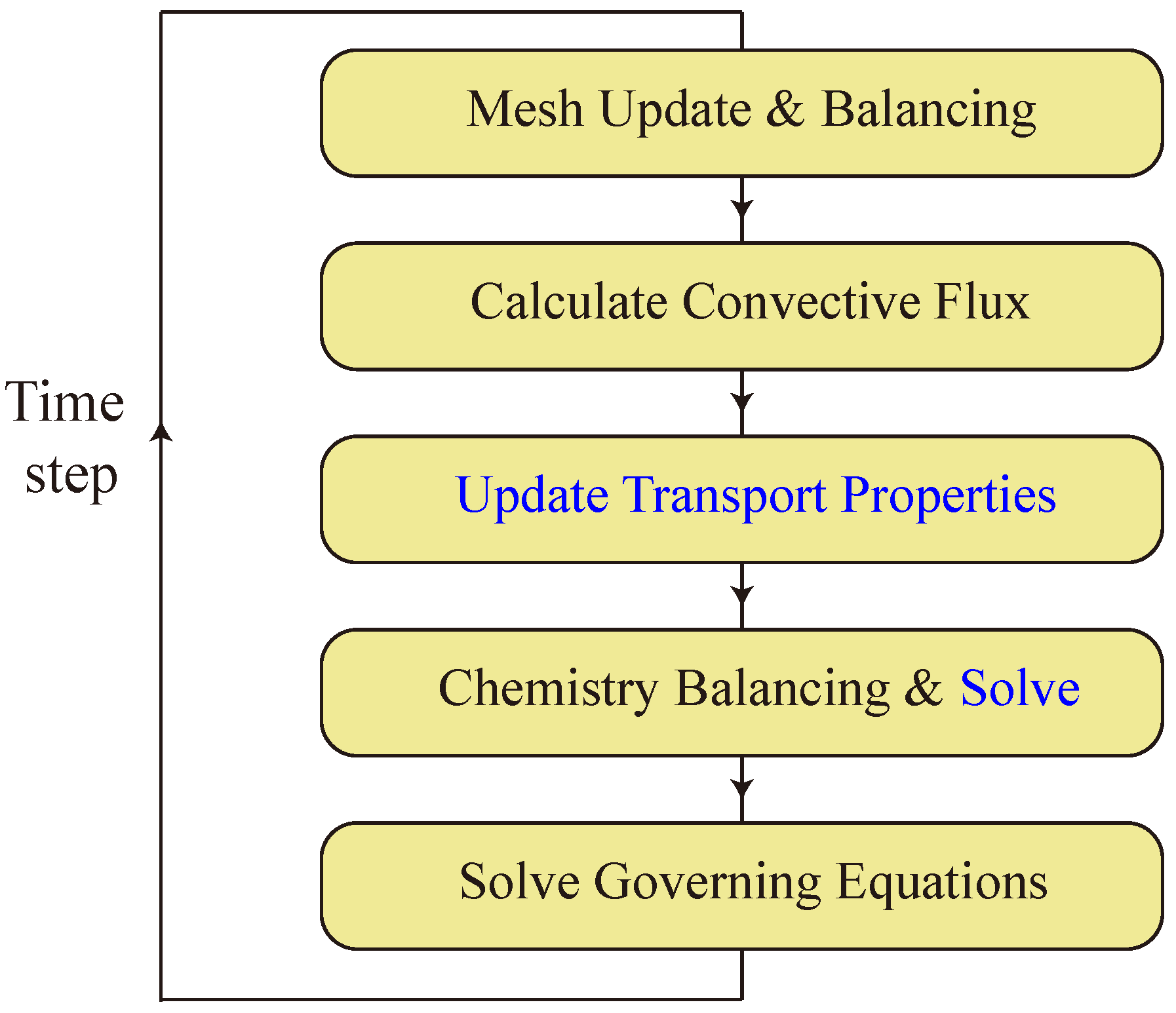
Funding

This research was funded by National Natural Science Foundation of China, grant number 52076003.

Institutional Review Board Statement

Not applicable.

Informed Consent Statement

Not applicable.

Data Availability Statement

The data that support the findings of this study are available from the corresponding author upon reasonable request.

Acknowledgments

Part of the computations in this work were supported by resources from the Beijing Super Cloud Computing Center (https://www.blsc.cn (accessed on 11 January 2024)). We also appreciate the contributions of the OpenFOAM and Cantera community.

Conflicts of Interest

The authors declare no conflicts of interest.

Abbreviations

The following abbreviations are used in this manuscript:
RDERotating detonation engine
CFDComputational fluid dynamics
RDCRotating detonation combustor
AMRAdaptive mesh refinement
DLBDynamic load balancing
0DZero-dimensional
1DOne-dimensional
2DTwo-dimensional
3DThree-dimensional
ODEOrdinary differential equation
ARCAnalytically reduced chemistry
NTCNegative temperature coefficient
CJChapman–Jouguet

Appendix A. Reaction Mechanism

The reduced C 12 H 23 /air mechanism from Liu [54] contains 18 species and 30 reactions, as listed in Table A1.
Table A1. Reduced C 12 H 23 /air mechanism units: [s, mol, cm 3 , kcal].
No.ReactionAn E a
1 C 12 H 23 + O 2 5 C 2 H 4 + C 2 H 3 + O 2 7.50 × 10 + 07 1.5015.701
2 C 12 H 23 + OH 6 C 2 H 4 + O2.00 × 10 + 07 1.0018.901
3H + O 2 OH + O3.52 × 10 + 16 −0.7017.056
4OH + O ⟶ H + O 2 1.15 × 10 + 14 −0.32−0.167
5OH + H 2 H 2 O + H1.17 × 10 + 09 1.303.631
6 H 2 O + H ⟶ OH + H 2 6.72 × 10 + 09 1.3020.209
7O + H 2 O OH + OH7.60 × 10 + 00 3.8412.780
8OH + OH ⟶ O + H 2 O 2.45 × 10 01 3.97−4.539
9 aH + O 2 + M HO 2 + M6.76 × 10 + 19 −1.400
10 HO 2 + H ⟶ OH + OH1.70 × 10 + 14 00.884
11 HO 2 + H H 2 + O 2 4.28 × 10 + 13 01.409
12 HO 2 + OH H 2 O + O 2 2.89 × 10 + 13 0−0.502
13 aH + OH + M H 2 O + M2.20 × 10 + 22 −2.000
14 a H 2 O + M ⟶ H + OH + M2.18 × 10 + 23 −1.93119.201
15CO + OH CO 2 + H4.40 × 10 + 06 1.50−0.741
16 CO 2 + H ⟶ CO + OH4.97 × 10 + 08 1.5021.428
17 C 2 H 4 + O 2 C 2 H 3 + HO 2 4.22 × 10 + 13 057.570
18 C 2 H 4 + OH C 2 H 3 + H 2 O 2.70 × 10 + 05 2.312.962
19 C 2 H 4 + O CH 2 CHO + H2.25 × 10 + 06 2.080
20 C 2 H 4 + O CH 3 + HCO1.21 × 10 + 06 2.080
21 C 2 H 4 + H C 2 H 3 + H 2 2.25 × 10 + 07 2.1213.353
22 C 2 H 3 + O 2 CH 2 O + HCO1.70 × 10 + 29 −5.316.498
23 C 2 H 3 + O 2 CH 2 CHO + O7.00 × 10 + 14 −0.615.255
24 CH 3 + O 2 CH 2 O + OH3.30 × 10 + 11 08.934
25 CH 3 + O CH 2 O + H8.43 × 10 + 13 00
26 CH 2 CHO CH 2 CO + H1.05 × 10 + 37 −7.1944.432
27 CH 2 CO + H CH 3 + CO1.11 × 10 + 07 2.002.007
28 CH 2 O + OH ⟶ HCO + H 2 O 3.90 × 10 + 10 0.890.406
29 bHCO + M ⟶ CO + H + M1.86 × 10 + 17 −1.0016.984
30HCO + O 2 CO + HO 2 3.00 × 10 + 12 00
a Third-body efficiencies: CO = 1.9, CO 2 = 3.8, H 2 = 2.5, H 2 O = 12.0; b Third-body efficiencies: CO = 2.5, CO 2 = 2.5, H 2 = 1.9, H 2 O = 12.0.

References

  1. Wolański, P. Detonative propulsion. Proc. Combust. Inst. 2013, 34, 125–158. [Google Scholar] [CrossRef]
  2. Kailasanath, K. Recent developments in the research on pressure-gain combustion devices. In Innovations in Sustainable Energy and Cleaner Environment; Springer: Singapore, 2020; pp. 3–21. [Google Scholar]
  3. Anand, V.; Gutmark, E. Rotating detonation combustors and their similarities to rocket instabilities. Prog. Energy Combust. Sci. 2019, 73, 182–234. [Google Scholar] [CrossRef]
  4. Ma, J.Z.; Luan, M.Y.; Xia, Z.J.; Wang, J.P.; Zhang, S.J.; Yao, S.B.; Wang, B. Recent progress, development trends, and consideration of continuous detonation engines. AIAA J. 2020, 58, 4976–5035. [Google Scholar] [CrossRef]
  5. Kindracki, J.; Wacko, K.; Woźniak, P.; Siatkowski, S.; Meżyk, Ł. Influence of gaseous hydrogen addition on initiation of rotating detonation in liquid fuel–air mixtures. Energies 2020, 13, 5101. [Google Scholar] [CrossRef]
  6. Bennewitz, J.W.; Bigler, B.R.; Ross, M.C.; Danczyk, S.A.; Hargus, W.A., Jr.; Smith, R.D. Performance of a rotating detonation rocket engine with various convergent nozzles and chamber lengths. Energies 2021, 14, 2037. [Google Scholar] [CrossRef]
  7. Han, H.S.; Lee, E.S.; Choi, J.Y. Experimental investigation of detonation propagation modes and thrust performance in a small rotating detonation engine using C2H4/O2 propellant. Energies 2021, 14, 1381. [Google Scholar] [CrossRef]
  8. Chen, Y.; Liu, X.; Wang, J. Effects of reversed shock waves on operation mode in H2/O2 rotating detonation chambers. Energies 2021, 14, 8296. [Google Scholar] [CrossRef]
  9. Liu, X.Y.; Chen, Y.L.; Xia, Z.J.; Wang, J.P. Numerical study of the reverse-rotating waves in rotating detonation engine with a hollow combustor. Acta Astronaut. 2020, 170, 421–430. [Google Scholar] [CrossRef]
  10. Betelin, V.; Nikitin, V.; Mikhalchenko, E. 3D numerical modeling of a cylindrical RDE with an inner body extending out of the nozzle. Acta Astronaut. 2020, 176, 628–646. [Google Scholar] [CrossRef]
  11. Nikitin, V.; Mikhalchenko, E. Safety of a rotating detonation engine fed by acetylene–oxygen mixture launching stage. Acta Astronaut. 2022, 194, 496–503. [Google Scholar] [CrossRef]
  12. Smirnov, N.; Nikitin, V.; Stamov, L.; Mikhalchenko, E.; Tyurenkova, V. Rotating detonation in a ramjet engine three-dimensional modeling. Aerosp. Sci. Technol. 2018, 81, 213–224. [Google Scholar] [CrossRef]
  13. Schau, K.A.; Oefelein, J.C. Numerical Analysis of Wave Characteristics in a Methane-Oxygen Rotating Detonation Engine. AIAA J. 2023, 61, 97–111. [Google Scholar] [CrossRef]
  14. Li, J.; Yu, J.; Li, J.; Lei, Y.; Yao, S.; Zhang, W. Investigation of hydrogen-enriched kerosene-fueled rotating detonation engine with multi-column film cooling. Phys. Fluids 2024, 36, 016138. [Google Scholar] [CrossRef]
  15. OpenFOAM. Available online: https://www.openfoam.com (accessed on 11 January 2024).
  16. Komen, E.; Camilo, L.H.; Shams, A.; Geurts, B.J.; Koren, B. A quantification method for numerical dissipation in quasi-DNS and under-resolved DNS, and effects of numerical dissipation in quasi-DNS and under-resolved DNS of turbulent channel flows. J. Comput. Phys. 2017, 345, 565–595. [Google Scholar] [CrossRef]
  17. Zirwes, T.; Zhang, F.; Habisreuther, P.; Hansinger, M.; Bockhorn, H.; Pfitzner, M.; Trimis, D. Quasi-DNS dataset of a piloted flame with inhomogeneous inlet conditions. Flow Turbul. Combust. 2020, 104, 997–1027. [Google Scholar] [CrossRef]
  18. Greenshields, C.J.; Weller, H.G.; Gasparini, L.; Reese, J.M. Implementation of semi-discrete, non-staggered central schemes in a colocated, polyhedral, finite volume framework, for high-speed viscous flows. Int. J. Numer. Methods Fluids 2010, 63, 1–21. [Google Scholar] [CrossRef]
  19. Kurganov, A.; Noelle, S.; Petrova, G. Semidiscrete central-upwind schemes for hyperbolic conservation laws and Hamilton–Jacobi equations. SIAM J. Sci. Comput. 2001, 23, 707–740. [Google Scholar] [CrossRef]
  20. Ettner, F.; Vollmer, K.G.; Sattelmayer, T. Numerical simulation of the deflagration-to-detonation transition in inhomogeneous mixtures. J. Combust. 2014, 2014. [Google Scholar] [CrossRef]
  21. Toro, E.F.; Spruce, M.; Speares, W. Restoration of the contact surface in the HLL-Riemann solver. Shock Waves 1994, 4, 25–34. [Google Scholar] [CrossRef]
  22. Marcantoni, L.G.; Tamagno, J.; Elaskar, S. rhoCentralRfFoam: An OpenFOAM solver for high speed chemically active flows–simulation of planar detonations–. Comput. Phys. Commun. 2017, 219, 209–222. [Google Scholar]
  23. Marcantoni, L.G.; Tamagno, J.; Elaskar, S. Two-dimensional numerical simulations of detonation cellular structures in h2o2ar mixtures with openfoam®. Int. J. Hydrogen Energy 2017, 42, 26102–26113. [Google Scholar] [CrossRef]
  24. Huang, Z.; Zhao, M.; Xu, Y.; Li, G.; Zhang, H. Eulerian-Lagrangian modelling of detonative combustion in two-phase gas-droplet mixtures with OpenFOAM: Validations and verifications. Fuel 2021, 286, 119402. [Google Scholar] [CrossRef]
  25. Xia, Z.J.; Sheng, Z.H.; Shen, D.W.; Wang, J.P. Numerical investigation of pre-detonator in rotating detonation engine. Int. J. Hydrogen Energy 2021, 46, 31428–31438. [Google Scholar] [CrossRef]
  26. Shen, D.; Cheng, M.; Wu, K.; Sheng, Z.; Wang, J. Effects of supersonic nozzle guide vanes on the performance and flow structures of a rotating detonation combustor. Acta Astronaut. 2022, 193, 90–99. [Google Scholar] [CrossRef]
  27. Rong, G.; Cheng, M.; Zhang, Y.; Sheng, Z.; Wang, J. Investigation of flow field characteristics and performance of carbon–hydrogen/oxygen-rich air rotating detonation engine. Phys. Fluids 2023, 35. [Google Scholar] [CrossRef]
  28. Hou, Y.; Cheng, M.; Sheng, Z.; Wang, J. Unsteady conjugate heat transfer simulation of wall heat loads for rotating detonation combustor. Int. J. Heat Mass Transf. 2024, 221, 125081. [Google Scholar] [CrossRef]
  29. Goodwin, D.G.; Speth, R.L.; Moffat, H.K.; Weber, B.W. Cantera: An Object-Oriented Software Toolkit for Chemical Kinetics, Thermodynamics, and Transport Processes. Version 2.5.1. 2021. Available online: https://cantera.org (accessed on 11 January 2024).
  30. Rettenmaier, D.; Deising, D.; Ouedraogo, Y.; Gjonaj, E.; De Gersem, H.; Bothe, D.; Tropea, C.; Marschall, H. Load balanced 2D and 3D adaptive mesh refinement in OpenFOAM. SoftwareX 2019, 10, 100317. [Google Scholar] [CrossRef]
  31. Scheufler, H. multiDimAMR. Available online: https://github.com/HenningScheufler/multiDimAMR (accessed on 11 January 2024).
  32. Tekgül, B.; Peltonen, P.; Kahila, H.; Kaario, O.; Vuorinen, V. DLBFoam: An open-source dynamic load balancing model for fast reacting flow simulations in OpenFOAM. Comput. Phys. Commun. 2021, 267, 108073. [Google Scholar] [CrossRef]
  33. Kee, R.J.; Coltrin, M.E.; Glarborg, P.; Zhu, H. Chemically Reacting Flow: Theory, Modeling, and Simulation; John Wiley & Sons: New York, NY, USA, 2017. [Google Scholar]
  34. Poling, B.E.; Prausnitz, J.M.; O’connell, J.P. The Properties of Liquids and Gases; McGraw-Hill: New York, NY, USA, 2001. [Google Scholar]
  35. Zheng, H.; Shu, C.; Chew, Y.T. An object-oriented and quadrilateral-mesh based solution adaptive algorithm for compressible multi-fluid flows. J. Comput. Phys. 2008, 227, 6895–6921. [Google Scholar] [CrossRef]
  36. Harten, A.; Lax, P.D.; Leer, B.v. On upstream differencing and Godunov-type schemes for hyperbolic conservation laws. SIAM Rev. 1983, 25, 35–61. [Google Scholar] [CrossRef]
  37. Chen, S.; Cai, F.; Xue, H.; Wang, N.; Yan, C. An improved AUSM-family scheme with robustness and accuracy for all Mach number flows. Appl. Math. Model. 2020, 77, 1065–1081. [Google Scholar] [CrossRef]
  38. Deiterding, R. Parallel Adaptive Simulation of Multi-Dimensional Detonation Structures. Ph.D. Thesis, Brandenburg University of Technology: Cottbus, Germany, 2003. [Google Scholar]
  39. Strang, G. On the construction and comparison of difference schemes. SIAM J. Numer. Anal. 1968, 5, 506–517. [Google Scholar] [CrossRef]
  40. Hindmarsh, A.C.; Brown, P.N.; Grant, K.E.; Lee, S.L.; Serban, R.; Shumaker, D.E.; Woodward, C.S. SUNDIALS: Suite of nonlinear and differential/algebraic equation solvers. ACM Trans. Math. Softw. (TOMS) 2005, 31, 363–396. [Google Scholar] [CrossRef]
  41. Kee, R.J.; Rupley, F.M.; Miller, J.A. Chemkin-II: A Fortran Chemical Kinetics Package for the Analysis of Gas-Phase Chemical Kinetics; Technical Report SAND-89-8009; Sandia National Lab: Livermore, CA, USA, 1989. [Google Scholar]
  42. Cazères, Q.; Pepiot, P.; Riber, E.; Cuenot, B. A fully automatic procedure for the analytical reduction of chemical kinetics mechanisms for computational fluid dynamics applications. Fuel 2021, 303, 121247. [Google Scholar] [CrossRef]
  43. Mcbride, B.J.; Gordon, S.; Reno, M.A. Coefficients for Calculating Thermodynamic and Transport Properties of Individual Species; Technical Report NASA-TM-4513; National Aeronautics and Space Administration: Cleveland, OH, USA, 1993.
  44. Bhagatwala, A.; Luo, Z.; Shen, H.; Sutton, J.A.; Lu, T.; Chen, J.H. Numerical and experimental investigation of turbulent DME jet flames. Proc. Combust. Inst. 2015, 35, 1157–1166. [Google Scholar] [CrossRef]
  45. Mehl, M.; Pitz, W.J.; Westbrook, C.K.; Curran, H.J. Kinetic modeling of gasoline surrogate components and mixtures under engine conditions. Proc. Combust. Inst. 2011, 33, 193–200. [Google Scholar] [CrossRef]
  46. Yang, Q.; Zhao, P.; Ge, H. reactingFoam-SCI: An open source CFD platform for reacting flow simulation. Comput. Fluids 2019, 190, 114–127. [Google Scholar] [CrossRef]
  47. Sod, G.A. A survey of several finite difference methods for systems of nonlinear hyperbolic conservation laws. J. Comput. Phys. 1978, 27, 1–31. [Google Scholar] [CrossRef]
  48. Quirk, J.J. A contribution to the great Riemann solver debate. Int. J. Numer. Methods Fluids 1994, 18, 555–574. [Google Scholar] [CrossRef]
  49. Kim, S.D.; Lee, B.J.; Lee, H.J.; Jeung, I.S. Robust HLLC Riemann solver with weighted average flux scheme for strong shock. J. Comput. Phys. 2009, 228, 7634–7642. [Google Scholar] [CrossRef]
  50. Law, C.K. Combustion Physics; Cambridge University Press: Cambridge, UK, 2010. [Google Scholar]
  51. Li, J.; Zhao, Z.; Kazakov, A.; Dryer, F.L. An updated comprehensive kinetic model of hydrogen combustion. Int. J. Chem. Kinet. 2004, 36, 566–575. [Google Scholar] [CrossRef]
  52. Grcar, J.F. The TWOPNT Program for Boundary Value Problems; Technical Report SAND91-8230; Sandia National Lab: Livermore, CA, USA, 1992. [Google Scholar]
  53. Sheng, Z.; Cheng, M.; Wang, J.P. Multi-wave effects on stability and performance in rotating detonation combustors. Phys. Fluids 2023, 35, 076119. [Google Scholar] [CrossRef]
  54. Liu, X. Numerical Investigations on the Stability and Thrust Performance of Rotating Detonation Engine. Ph.D. Thesis, Peking University, Beijing, China, 2023. (In Chinese). [Google Scholar]
  55. Shepherd, J. Shock & Detonation Toolbox. Available online: https://shepherd.caltech.edu/EDL/PublicResources/sdt (accessed on 11 January 2024).
  56. Oran, E.S.; Weber, J.W., Jr.; Stefaniw, E.I.; Lefebvre, M.H.; Anderson, J.D., Jr. A numerical study of a two-dimensional H2-O2-Ar detonation using a detailed chemical reaction model. Combust. Flame 1998, 113, 147–163. [Google Scholar] [CrossRef]
  57. Wang, C.; Xu, S.; Guo, C. Gaseous detonation propagation in a bifurcated tube. J. Fluid Mech. 2008, 599, 81–110. [Google Scholar] [CrossRef]
  58. Poinsot, T.J.; Lelef, S.K. Boundary conditions for direct simulations of compressible viscous flows. J. Comput. Phys. 1992, 101, 104–129. [Google Scholar] [CrossRef]
  59. Smirnov, N.; Betelin, V.; Nikitin, V.; Stamov, L.; Altoukhov, D. Accumulation of errors in numerical simulations of chemically reacting gas dynamics. Acta Astronaut. 2015, 117, 338–355. [Google Scholar] [CrossRef]
  60. Smirnov, N.; Betelin, V.; Shagaliev, R.; Nikitin, V.; Belyakov, I.; Deryuguin, Y.N.; Aksenov, S.; Korchazhkin, D. Hydrogen fuel rocket engines simulation using LOGOS code. Int. J. Hydrogen Energy 2014, 39, 10748–10756. [Google Scholar] [CrossRef]
  61. Ó Conaire, M.; Curran, H.J.; Simmie, J.M.; Pitz, W.J.; Westbrook, C.K. A comprehensive modeling study of hydrogen oxidation. Int. J. Chem. Kinet. 2004, 36, 603–622. [Google Scholar] [CrossRef]
  62. Mahmoudi, Y.; Mazaheri, K.; Parvar, S. Hydrodynamic instabilities and transverse waves in propagation mechanism of gaseous detonations. Acta Astronaut. 2013, 91, 263–282. [Google Scholar] [CrossRef]
Figure 1. Flow chart within a time step Δ t F in BYCFoam. Calculations carried out in Cantera are denoted by the blue font.
Energies 17 00769 g001
Figure 2. Specific heat capacity c p of stoichiometric DME/air mixtures.
Energies 17 00769 g002
Figure 3. Homogeneous autoignition of stoichiometric DME/air mixtures: (a) ignition delay time with different initial temperatures T 0 and initial pressures P 0 , (b) temperature evolution during autoignition with T 0 = 625 K and P 0 = 0.5 atm.
Energies 17 00769 g003
Figure 4. Solutions of 1D Sod shock-tube problem at time t = 0.15 : (a) pressure, (b) density. Black solid line: Riemann exact solution. Red solid line: rhoCentralFoam. Dashed lines: BYCFoam with four flux schemes.
Energies 17 00769 g004
Figure 5. The close-up of (a) pressure distributions behind the shock wave; (b) density distributions near the contact discontinuity. Black solid line: Riemann exact solution. Red solid line: rhoCentralFoam. Dashed lines: BYCFoam with four flux schemes.
Energies 17 00769 g005
Figure 6. Density contours of shock-wave diffraction.
Energies 17 00769 g006
Figure 7. Temperature evolution during autoignition with three different solvers (a) DME/air (b) n-heptane/air.
Energies 17 00769 g007
Figure 8. Laminar flame speeds of premixed hydrogen/air mixture with varying equivalence ratios.
Energies 17 00769 g008
Figure 9. One-dimensional planar flame structure of stoichiometric hydrogen/air mixture: (a) temperature and density, (b) mass fraction of O H and H 2 O 2 .
Energies 17 00769 g009
Figure 10. Numerical simulation of one-dimensional detonation tube with kerosene/air mixture at 1 atm and 373 K: (a) schematic of the detonation tube, (b) temperature and pressure distributions at different simulation times.
Energies 17 00769 g010
Figure 11. The computational domain and initial setup in the simulation of a detonation cellular structure.
Energies 17 00769 g011
Figure 12. The final flow fields of a mode-four detonation: (a) pressure, (b) temperature, (c) mesh refinement, (d) mass fraction of O H .
Energies 17 00769 g012
Figure 13. Numerical simulation of a two-dimensional detonation cellular structure: (a) schlieren plot by density gradient, (b) triple-point trajectories.
Energies 17 00769 g013
Figure 14. Schematic of an RDC in a two-dimensional computational domain.
Energies 17 00769 g014
Figure 15. Schematic of the initial conditions. A hot spot is located at the bottom of the computational domain to ignite the reactants. The rest of the mixture is air at 1 atm and 300 K.
Energies 17 00769 g015
Figure 16. The mass flow rates of the inlet and outlet. Solid lines: Case 0 with a static mesh. Dashed lines: Case 5 with AMR.
Energies 17 00769 g016
Figure 17. The well-developed flow fields of an RDC. (a) Temperature and (b) mass fraction of O H in Case 0. (c) Temperature and (d) mass fraction of O H in Case 5. (e) Temperature and pressure distributions in the circumferential direction at y = 0.2 cm. Solid lines: Case 0 with static mesh. Dashed lines: Case 5 with AMR.
Energies 17 00769 g017
Table 1. The distinctions between rhoCentralFoam and BYCFoam.
SolverReconstruction VariablesFlux Schemes
rhoCentralFoam( ρ ,   ρ u ,   R T ,   e ,   c ) *Kurganov
BYCFoam( ρ ,   u ,   p )Kurganov, HLL, HLLC, AUSM+M
* c is sound speed.
Table 2. Initial conditions of auto-ignition.
FuelInitial Temperature [K]Initial Pressure [atm]Chemical Mechanisms
DME6501Bhagatwala et al. [44]
n-heptane7003LLNL (Version 3) [45]
Table 3. Comparisons of one-dimensional detonation properties with varying equivalence ratios ϕ . U is the detonation velocity, p and T are the pressure and temperature at the CJ points of the detonation wave, respectively. e r r is the maximum relative error between 1D simulations and the theoretical CJ properties of ( U ,   p ,   T ).
ϕ U CJ [m/s] U Sim [m/s] p CJ [atm] p Sim [atm] T CJ [K] T Sim [K] err
0.81723.711716.2413.6713.512709.562703.751.17%
1.01795.041789.3115.0714.942876.972880.140.86%
1.21830.441827.9315.7315.682913.652906.930.32%
1.41832.181822.0615.6715.482828.182822.311.21%
Table 4. Refinement criteria used in the simulation of the detonation cellular structure.
CriteriaRefined Regions
ϵ ρ > 0.04 or 0.01Leading shock, transverse waves and slip lines
Y H 2 > 0.0027 and T > 1000 KInduction zone and reaction zone
Table 5. Comparisons of the detonation cell size with other numerical results. L and λ are the length and the width of the detonation cells, respectively.
StudyBase Grid [µm]Finest Grid [µm]Cell Size [mm]Comments
Δ x × Δ y Δ x × Δ y L × λ
Current study 200 × 200 25 × 25 53 × 30 AMR
Deiterding et al. [38] 500 × 750 31.250 × 46.875 53 × 30 AMR
Oran et al. [56] 150 × 235 - 54 × 31 Uniform grids
Wang et al. [57] 150 × 235 - 54 × 30 Uniform grids
Table 6. Test cases for the AMR and DLB algorithms. Case 0 is a benchmark without using any acceleration methods. Cases 0–1 are calculated with uniform static grids. Cases 2–5 are calculated with AMR. The CPU time costs in the computations are listed with a relative form.
CaseBase Grid [mm]Finest Grid [mm]DLB_MeshDLB_ChemRelative CPU Time
00.1---100%
10.1--80%
20.40.1--63%
30.40.1-20%
40.40.1-14%
50.40.111%
Disclaimer/Publisher’s Note: The statements, opinions and data contained in all publications are solely those of the individual author(s) and contributor(s) and not of MDPI and/or the editor(s). MDPI and/or the editor(s) disclaim responsibility for any injury to people or property resulting from any ideas, methods, instructions or products referred to in the content.

