Assessing the Wind Power Potential in Naama, Algeria to Complement Solar Energy through Integrated Modeling of the Wind Resource and Turbine Wind Performance

Abstract

In the context of the escalating global climate crisis and the urgent need for sustainable energy solutions, this study explores the integration of wind energy as a supplementary source to solar photovoltaic energy in Naama, Algeria. The research utilizes a decade-long anemometric dataset, along with concurrent solar radiation data, to investigate the potential of harnessing wind energy, particularly during periods of low solar irradiance. Employing advanced statistical methods, including the Weibull distribution, the study assesses the wind power generation potential of a 2 kW/day turbine. The research highlights an average evening increase in wind speeds, which inversely correlates with the diminished solar energy production after sunset. This seasonal pattern is further substantiated by a significant negative correlation between wind speed and solar radiation for most of the year (January to May and September to December), with Pearson coefficients ranging from −0.713 to −0.524 (p < 0.05). However, the study also notes an absence of a notable correlation during the summer months (June to August) attributed to seasonal wind variations and the peak of solar irradiance. These findings confirm Naama as an ideal location for integrated renewable energy systems, thereby demonstrating the natural synergy between solar and wind energy. This synergy is particularly effective in mitigating the intermittency of solar power, thus highlighting the potential of wind energy during periods of low solar activity.

1. Introduction

The global energy landscape is undergoing a profound transformation driven by the urgent imperative to reduce carbon emissions in the face of escalating climate change concerns. This significant shift is largely driven by acknowledging the unsustainable nature of prolonged dependence on fossil fuels. Within this transition, renewables have emerged as critical solutions, with solar power taking a leading role. Algeria, boasting significant solar resources, is strategically positioning itself as a key player in extensive photovoltaic deployment through its commitment to active energy mix diversification and carbon footprint reduction [1]. However, this transition encounters major challenges, particularly the intermittent nature of solar energy. Such variability can lead to substantial challenges, particularly in countries like Algeria where solar is expected to constitute a significant portion of the energy mix. In striving for a consistent and reliable electricity supply, the necessity for complementary solutions to address these inherent fluctuations in renewable sources has become increasingly evident [2]. Theoretical models support that combining solar energy with other sources, which have noncorrelated generation profiles, can effectively reduce this variability. The concept of hybrid systems, therefore, presents significant integration synergies by exploiting the complementary characteristics of different renewable resources [3].

Wind power, as a supplementary source, offers a compelling solution, especially in regions where wind and solar patterns are inversely correlated. The desert province of Naama is a prime example of such an environment, which often exhibits increased wind speeds during periods of lower solar radiation. This advantageous climatic feature presents a unique opportunity for leveraging the synergistic potentials of wind and solar, thereby effectively reducing their variability. Advanced modeling has demonstrated that hybrid wind–solar systems possess significant capabilities to balance the inherent variability of each renewable energy source. By employing geospatial optimization and intelligent operational strategies, these multitechnology systems can achieve enhanced capacity factors and improved reliability [4]. Yet, fully harnessing the capabilities of such systems poses considerable challenges. Optimizing the configuration of solar and wind assets requires a detailed analysis of resource complementarity across various timescales. Managing and integrating these variable generation profiles to meet grid demands is a technically intricate task. Moreover, the development of suitably designed storage systems, advanced forecasting tools, and robust transmission infrastructure is crucial [5]. However, overcoming these obstacles is feasible through comprehensive technoeconomic modeling, the application of proven control technologies, and strategic system planning [6].

This study’s twin objectives are the following: first, to quantify the exploitable wind resources in Naama during periods of reduced solar insolation and, second, to evaluate the potential of wind energy in counterbalancing solar intermittency. Furthermore, this research introduces an innovative analytical methodology, focusing on a combined assessment of solar and wind patterns, to elucidate their temporal complementarity [7]. While prior work has established techniques utilizing statistical approaches and simulation tools, this research aims to further refine the methodology through the analysis of high-resolution, on-site data. The approach involves a detailed statistical analysis of long-term anemometric data from Naama. By applying Weibull distribution fitting, the probability distributions of wind speed were modeled, thereby facilitating the determination of theoretical power potential. The study also examines correlations between wind speeds and solar insolation across different timescales with the aim to quantify the wind’s contribution during periods of reduced solar activity. Precisely characterizing the complementarity of renewable resources through statistical correlations is vital for the optimization of hybrid energy systems [8]. This study strives to determine a substantial inverse correlation between hourly average wind speeds and irradiation. In doing so, it evaluates the potential of wind power to support solar generation, particularly in the evenings when photovoltaic output naturally declines. Additionally, the research develops a versatile statistical framework that can be adapted for other regions exploring hybrid wind–solar platforms [9].

The results offer convincing evidence of wind power’s viability in stabilizing Naama’s intermittent solar resources. These findings have significant implications for renewable energy planning in Algeria and in similar environments [10,11]. Adopting an integrated approach that harnesses both resources is recommended and in line with global sustainability goals. Overall, the study presents an exemplary methodology and reiterates the potential of hybrid systems in delivering affordable, low-carbon power generation. As the share of variable renewables expands globally, innovative solutions for managing variability will become increasingly important [11].

2. Materials and Methods

2.1. Mathematical Model

Integrating various renewable energy technologies into hybrid systems can markedly enhance power production and boost overall reliability. Each technology contributes a distinct generation profile. Strategically combining these profiles can lead to complementary and synergistic effects, thereby optimizing energy output. Solar photovoltaics (PVs) are especially effective in capturing energy during daylight hours, thereby offering a plentiful power source when the sun is out. However, their major limitation becomes apparent at night, when the absence of solar irradiance leads to zero output. This limitation highlights the need for a complementary energy source. In this scenario, wind energy emerges as a valuable ally. Wind patterns, often differing from solar energy patterns, exhibit unique hourly and seasonal fluctuations. Such variations in wind energy can be advantageous, thus often aligning perfectly with times when solar energy is not available. For example, in many regions, wind speeds increase during the evening or at night, which is precisely when solar PV systems stop producing energy [12,13].

The incorporation of wind power into a solar generation system results in a more robust and reliable energy solution. A critical aspect is ensuring that wind resources are strong during the evening and other periods when solar power is not available. This synergistic relationship between wind and solar power not only optimizes energy production efficiency but is also pivotal in building a sustainable and reliable renewable energy infrastructure.

To quantify this, the total generated power (P) for a wind–solar hybrid system can be mathematically modeled:

$$\begin{array}{c}\hfill \begin{array}{c}P=P_{PV}+P_{Wind}\hfill \end{array}\end{array}$$

(1)

In a hybrid renewable energy system, ‘PPV’ indicates the output from solar photovoltaics, and ‘PWind’ represents the output from wind turbines. The success and practicality of such a system largely depend on how well the solar and wind resources correlate. Ideally, these resources should exhibit negatively correlated generation profiles, with wind patterns effectively offsetting solar variability. This ensures efficient integration and maximizes energy production efficiency [1].

To determine the power output ($P_{PV}$) of a solar photovoltaic array, it is essential to consider various factors, including the following:

$$\begin{array}{c}\hfill \begin{array}{c}{P}_{PV}=f_{PV}\ast A\ast r\ast H\hfill \end{array}\end{array}$$

(2)

In this context, $f_{PV}$ represents the efficiency of the photovoltaic system, A denotes the total area covered by solar panels, r stands for the solar irradiance measured in watts per square meter (W/m²), and H signifies the number of daylight hours. Solar irradiance, which depends on both location and weather conditions, is available exclusively during daylight hours.

Concerning the power output ($P_{Wind}$) of a wind turbine, it is typically modeled using the following formula [14]:

$$\begin{array}{c}\hfill \begin{array}{c}{\displaystyle P_{wind}=\left(\frac{1}{2}\right)\ast \rho \ast A\ast V^3\ast C_p}\hfill \end{array}\end{array}$$

(3)

where $\rho$ represents the air density, A indicates the swept area of the turbine blades, V refers to the wind speed, and $C_p$ is the power coefficient. Wind patterns show fluctuations on an hourly and seasonal basis, which are influenced by both weather conditions and the local climate. By combining Equations (2) and (3), we arrive at the total power, P, generated by the hybrid system. This integration effectively merges the distinct characteristics of solar and wind energy production, thus taking into account the variables from both renewable sources to calculate the system’s overall power output.

This method of calculation recognizes the inherent variability in both solar and wind energy, thereby providing a more comprehensive and realistic assessment of the hybrid system’s performance. Consequently, this combined equation plays a crucial role in illustrating how these two renewable energy sources can complement each other, thereby improving the overall efficiency and reliability of the system [15].

$$\begin{array}{c}\hfill \begin{array}{c}{\displaystyle P=f_{PV}\ast A\ast r\ast H+\left(\frac{1}{2}\right)\ast \rho \ast A\ast V^3\ast C_p}\hfill \end{array}\end{array}$$

(4)

This study assessed whether Naama, a town in Algeria, possesses wind resources capable of supplementing evening power production to compensate for the decline in solar photovoltaic output after sunset. Renowned for its exceptional solar potential, Naama possesses a mean irradiance of 5.5 kWh/m²/day, which has catalyzed substantial expansion in solar photovoltaic deployments. However, the absence of photovoltaic generation during the night, coupled with rising electricity demand, leads to daily power supply shortfalls [16]. To address this issue, local wind patterns in Naama were scrutinized using a decade’s worth of hourly wind speed data. This analysis aimed to determine whether these patterns could effectively complement solar variability and bridge the production gap during evening hours. A key part of this evaluation involved examining the relationship between wind speeds and the decrease in solar irradiance during sunset periods. This analysis is crucial for assessing the viability of an optimized hybrid wind–solar system. To gauge the complementary nature of wind and solar resources, correlation coefficients were calculated. Among these, the Pearson correlation coefficient, denoted as $\rho$, is commonly employed. The Pearson coefficient, a key measure in this analysis, is defined as follows:

$$\begin{array}{c}\hfill \begin{array}{c}{\displaystyle \rho \left(X,Y\right)=\frac{cov\left(X,Y\right)}{{\sigma }_x{\sigma }_y}}\hfill \end{array}\end{array}$$

(5)

This passage outlines the application of statistical measures and predictive models in optimizing the performance of hybrid solar–wind energy systems. Covariance (cov(X, Y)) and standard deviations ($\sigma$X and $\sigma$Y) were employed to understand the interrelation between solar and wind energy outputs. These statistical tools assist in analyzing the concurrent variability of these two energy sources. For forecasting future energy outputs, the text recommends utilizing time series forecasting models. It discusses two types: statistical models such as the autoregressive integrated moving average (ARIMA) and machine learning algorithms, including random forests. These models are instrumental in predicting future values of solar photovoltaic output (PPPV) and wind power output (PWind), thus drawing on historical data. The ARIMA model is particularly noted for its efficacy in forecasting time series data, especially when the data points are affected by their historical values. However, the specific mathematical structure or parameters of the ARIMA model are not detailed in the text. In summary, these predictive models play a crucial role in the efficient management of hybrid solar–wind systems. They facilitate the accurate forecasting of energy outputs, thus culminating in more dependable and effective energy management.

$$\begin{array}{c}\hfill \begin{array}{c}{X}_t={\varphi }_1.t^{-1}+{\varphi }_2.t^{-2}+\cdots +{\varphi }_p.t^{-p}+{\theta }_1.{ϵ}^{t-1}+\cdots +{\theta }_q.ϵt^{-q}+{ϵ}_t\hfill \end{array}\end{array}$$

(6)

In the ARIMA model, $X_t$ represents the value of the time series at time t, $\varphi$ and $\theta$ are model parameters that need to be estimated, and $\epsilon$ is the error term. These elements are crucial for accurately forecasting future values, as they account for past and current data, along with any randomness or unpredictability in the data series. The study’s main objective is to explore the temporal complementarity between solar and wind energy resources in the region. This involves assessing the correlation between solar and wind power and predicting their future outputs. A significant focus of the study is to determine if there is a noticeable increase in wind speeds and potential wind power output during the evening compared to daylight hours. If this is true, it would suggest that the wind resources in Naama could adequately compensate for the lack of solar power production when the sun is not available. Establishing the presence of strong evening wind potential would be a key factor in supporting the economic viability of integrating wind power with solar infrastructure. This integration strives to offer renewable power continuously throughout the day, thus significantly enhancing the region’s energy sustainability and reliability [17].

2.2. Site Description

Geographically, Naama, a region located in the southwest of Algeria, encompasses a vast area of 27,950 square kilometers. It is home to a population of around 200,000 inhabitants. This arid region is characterized by hot and dry conditions prevailing during the summer months and mild, occasionally rainy winters typical of desert environments [18]. In terms of geographic positioning, it is strategically positioned on an elevated plateau averaging 800 m above sea level; Naama’s geographical location contributes to its distinct climate and environmental conditions. The landscape is predominantly flat and interspersed with sparse grasslands; it features desert regions, occasional low hills, and rocky outcrops. Due to the harsh climatic conditions, vegetation in the area is limited and primarily comprises shrubs and hardy plant species adapted to withstand drought [18]. Climatically speaking, in terms of climate classification, Naama falls under the BWh category of the Köppen system, which denotes a desert climate. This is defined by extremely hot, prolonged summers and short, relatively warm winters. Statistically, the average annual temperature hovers around 21.2 $°$C. Temperatures vary widely, with July typically being the hottest month, when average highs can soar to around 41.4 $°$C. Conversely, January is usually the coldest month, with average lows dipping to approximately 3.8 $°$C [19]. The region receives very little rainfall, thus averaging about 130 mm annually. This scant precipitation is mostly concentrated in the winter months spanning November to March. The rainfall in Naama is characterized by brief, intense storms rather than steady downpours. Summers are notably devoid of rain, and the combination of low humidity and high solar radiation results in extremely high evaporation rates.

With regard to wind conditions in the region, the winds in Naama primarily originate from northerly and westerly directions. The region is often affected by sandstorms and dust storms, particularly during the spring season. Wind speeds tend to peak in June, thereby reaching average speeds of around 11mph. An interesting feature of Naama’s winds is the significant diurnal variation, where mornings typically experience calmer winds, while afternoons and evenings see stronger gusts.

Given its unique geographical and climatic attributes, the choice of Naama as a prime site for renewable energy projects, especially solar power, is driven by its extreme arid desert climate of hot summers, mild winters, and minimal rainfall. These conditions present abundant potential for solar energy harvesting. However, the region faces challenges due to inadequate electricity infrastructure and frequent power shortages. Developing renewable energy projects in this remote region provides an opportunity to more effectively meet local energy demand. Leveraging the area’s natural resources, such as plentiful sunshine and favorable wind patterns, can significantly enhance Naama’s energy independence and sustainability. Integrating renewable solar and wind power sources could provide a reliable, continuous power supply throughout the day, thereby addressing existing challenges and contributing to Naama’s overall economic and environmental well-being [20].

Delving into Algeria’s wind resources Figure 1, analysis shows the distribution of average wind speeds countrywide in meters/second at varying elevations. Significantly, Figure 1 depicts 80 m and 10 m elevations that highlight the Naama region’s prime potential for wind power. Its elevated plateau and arid climate provide steady, robust wind currents, which are ideal for harnessing wind energy. Additionally, with high solar irradiation and clear skies, Naama has substantial solar capabilities alongside its considerable wind assets. This dual solar and wind potential underscores Naama’s selection as a strategic site. By fully leveraging these complementary natural resources, Naama could play a pivotal role in spearheading Algeria’s transition to sustainable, renewable energy and diversifying its energy mix while cutting fossil fuel dependence. Thereby, Naama would meaningfully contribute to Algeria’s energy matrix and sustainability objectives [18].

Situated in the strategic Naama region Figure 2, the Salhi Ahmed Naama University Center stands out for its exceptional experimental capabilities in renewable energy research. Notably, it houses a state-of-the-art laboratory, led by experts, specializing in wind and solar technologies. A key asset is the lab’s sophisticated instrumentation collecting real-time, granular data on instant wind speeds—which is vital for advancing wind power solutions and optimizing turbine performance. Additional examples demonstrate the lab’s capabilities and leadership in leveraging Naama’s renewable potential through impactful research [21]. Therefore, the Center makes valuable contributions to renewable energy development, which are aligned with national objectives [22].

2.3. Solar and Wind Analysis for Energy Production Modeling

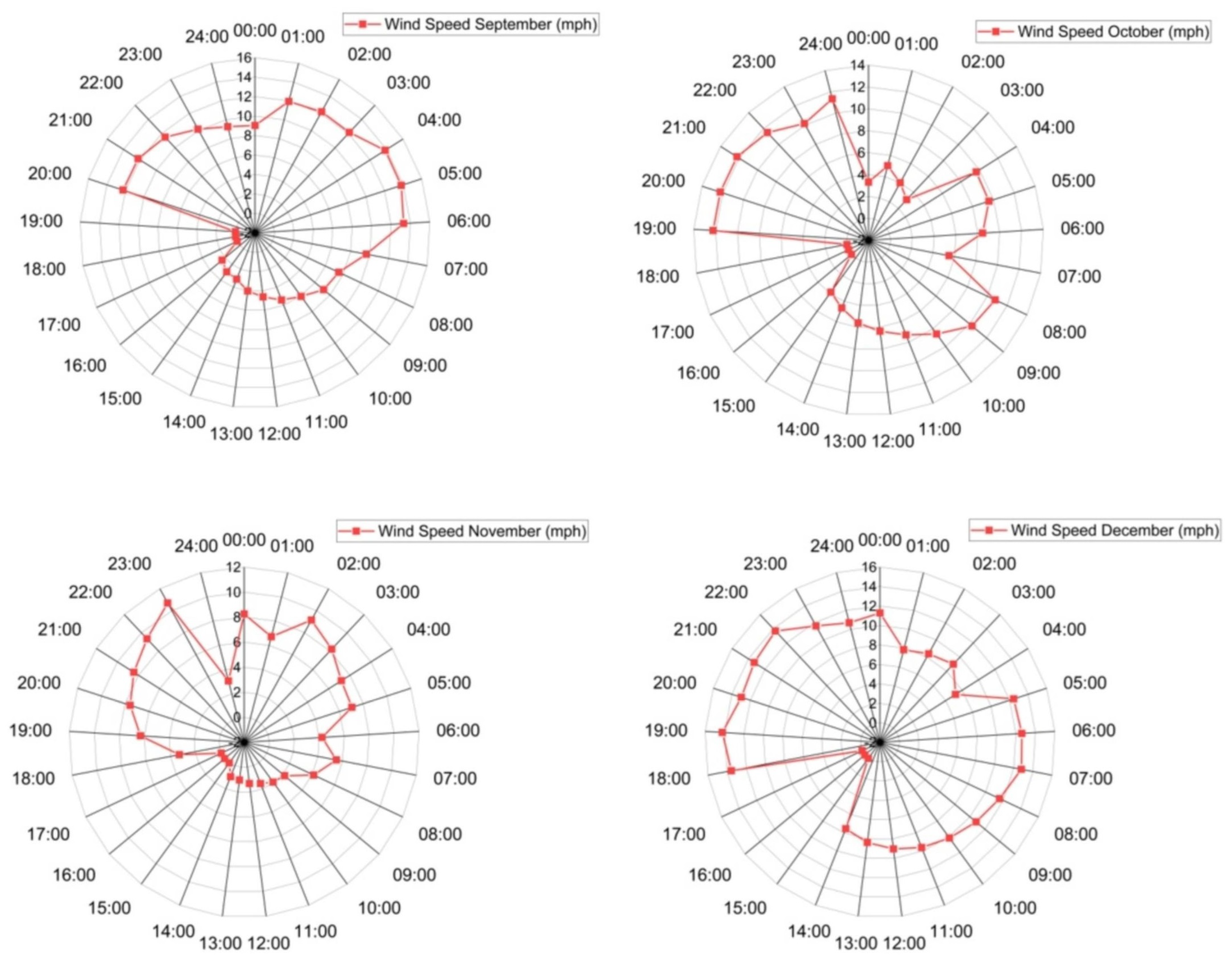
2.3.1. Exploratory Wind Data Analysis

The assessment of wind resources in Naama, Algeria required comprehensive analysis of historical wind data from 2012–2022 [23]. This dataset was obtained from meteorological instruments at Naama’s University Center, including cup anemometers and wind vanes at 10 m, 30 m, and 50 m elevations. These captured wind speeds and directions at 1Hz frequency, which were averaged over 10 min intervals [24].

Rigorous quality control measures were employed to ensure data integrity and accuracy. Values exceeding thresholds were excluded, and the dataset was closely examined for sensor issues and icing events; anomalies were corrected via inspection and crossheight correlation. Gaps up to 2 h were addressed through linear interpolation. The resulting refined decade-long Naama dataset underpinned subsequent wind distribution modeling [25].

Analysis of the validated 10 min average wind speed dataset over a decade incorporated graphical and statistical methodologies to elucidate the wind speeds’ inherent properties [24]. Time series visualizations across varying timescales highlighted seasonal and diurnal wind pattern shifts. Statistical indices like mean, standard deviation, minimum, maximum, median, mode, skewness and kurtosis encapsulated the velocity distribution traits. Additionally, quantile–quantile plots compared observed data against standard theoretical distributions to assess congruence. Preliminary examination revealed a pronounced Weibull distribution marked by a unimodal shape and positive skew, thereby indicating higher occurrence of lower wind speeds [23,25]. Data were then aggregated hourly and monthly to establish a foundation for more complex distribution modeling.

The assessment of wind resources in Naama Figure 3, Algeria entailed a comprehensive analysis of historical wind speed data recorded from 2012 to 2022 [23]. This dataset was derived from meteorological instruments positioned at the University Center of Naama city, thereby encompassing cup anemometers and wind vanes situated at elevations of 10 m, 30 m, and 50 m. These devices captured wind velocities and directions at a one-hertz frequency, which were subsequently averaged over ten-minute intervals to synthesize a more tractable dataset [24].

To ensure the data’s integrity and precision, rigorous quality control measures were employed. Values surpassing pre-established thresholds were identified and excluded from the analysis. Furthermore, the dataset was meticulously scrutinized for sensor malfunctions and icing occurrences, with anomalies rectified through manual inspection and crossheight correlation. Linear interpolation was utilized to bridge gaps in data continuity, which spanned up to two hours [25]. Subsequent to these refinements, the resulting decade-long dataset from Naama underpinned subsequent wind distribution modeling efforts [23].

2.3.2. Weibull Distribution Fitting

The Weibull probability density function was applied with meticulous precision to a comprehensive dataset spanning ten years of wind speed records, thereby effectively delineating the long-term frequency distribution of wind velocities [26]. This function can be expressed mathematically as follows:

$$\begin{array}{c}\hfill \begin{array}{c}{\displaystyle f(V,k,c)=\frac{c}{k}.{\left({\displaystyle \frac{V}{c}}\right)}^{k-1}.e^{-{\left({\displaystyle \frac{V}{c}}\right)}^k}}\hfill \end{array}\end{array}$$

(7)

where V denotes the wind speed, k denotes the shape factor, and c denotes the scale factor [27]. These parameters are pivotal in shaping the overall character of the distribution. For the determination of the most precise values of k and c, maximum likelihood estimation was employed, which is renowned for its accuracy in parameter estimation to achieve the optimal data fitting [28]. The mean wind speed, a critical element in wind energy analysis, correlates with these parameters as follows:

$$\begin{array}{c}\hfill \begin{array}{c}\mu =c\beta \left({\displaystyle 1+\frac{1}{k}}\right)\hfill \end{array}\end{array}$$

(8)

The average wind speed is calculated utilizing the beta function, which is denoted as B. This mathematical relation makes it possible to express the average wind speed as a function of the Weibull parameters k and c. The Weibull distribution has particular utility in wind energy applications, where it models the frequency of wind speeds that are crucial for estimating wind turbine power production. The model’s precision was rigorously evaluated using goodness-of-fit metrics such as R-squared, root-mean-square error, and chi-squared test statistics. Additionally, the Weibull cumulative distribution function is formulated as follows:

$$\begin{array}{c}\hfill \begin{array}{c}F\left(V,k,c\right)=1-e^{{\left({\displaystyle \frac{V}{c}}\right)}^k}\hfill \end{array}\end{array}$$

(9)

which was integrated to yield quartiles, exceedance probabilities, and quantile estimations, thus providing a comprehensive portrayal of wind speed distribution [26]. The analytical expressions for mean and variance, dependent on k and c, are specifically defined as follows:

$$\begin{array}{c}\hfill \begin{array}{c}\begin{array}{c}{\sigma }^2=c^2\left[\beta \left({\displaystyle 1+\frac{2}{k}}\right)-{\left(\beta \left({\displaystyle 1+\frac{1}{k}}\right)\right)}^2\right]\hfill \end{array}\hfill \end{array}\end{array}$$

(10)

which were employed to calculate the central tendency and dispersion of wind speeds. Segmenting the distributions monthly highlighted the seasonal variations in wind patterns, which are essential for understanding and forecasting fluctuations in energy production. Lastly, to address uncertainties in long-term wind speed analysis, uncertainty bounds for k and c were established, which were derived from subsamples of the decade-long dataset, thus ensuring robust and reliable parameter estimation.

The integration of the Weibull cumulative distribution function Figure 4 was instrumental in deriving quartiles, exceedance probabilities, and quantile estimates. Analytical formulas for mean and variance, dependent on the parameters k and c, enabled precise calculations of the data’s central tendency and dispersion. Seasonal variations were captured by segmenting the distributions monthly. Furthermore, to mitigate uncertainties in long-term analysis, bounds for k and c were determined from subsamples collected over the decade [29].

2.3.3. Statistical Study of Wind Speeds at the Naama Site

Over a decade of detailed research in Naama has provided deep insights into local wind behavior. Central to our analysis was the median wind speed, which offered stability against extreme data variations Figure 5, Figure 6 and Figure 7. Complementing this, we assessed wind variability through standard deviation and coefficient of variation, which are key in gauging both consistency and predictability—crucial aspects for project feasibility.

Our study also focused on the frequency and severity of extreme wind events. This data are essential for incorporating gust factors in turbine design, thereby prioritizing durability and safety. By employing Weibull and Rayleigh distributions, as well as precisely fitting their shape and scale factors, we captured a detailed picture of wind frequency patterns.

Power density analysis, conducted using cubic calculations, was instrumental in estimating the energy yield per unit area—a vital metric in evaluating wind resources. Wind roses, illustrating prevailing directions, enhanced our understanding of wind patterns, thereby assisting in identifying optimal turbine placements based on speed–direction correlations.

In a broader context, our initial findings revealed that average wind speeds peaked at 10–14 mph during autumn and spring and intensified during low solar irradiation periods—early mornings, evenings, and nights. This pattern suggests a potential inverse relationship between solar exposure and wind activity.

However, confirming this relationship demands more than preliminary observations. While current data point towards this link, only detailed, quantitative analysis can substantiate it. Advanced analytical techniques are necessary to determine if a significant correlation exists between reduced sunlight and increased wind speeds.

Table 1 summarizes the goodness-of-fit for Weibull and Rayleigh distributions and provides a comparative perspective, thereby anchoring our comprehensive approach. This extensive study of Naama’s wind patterns not only enhances our understanding but also lays a foundation for optimizing wind energy engineering [30].

The results of the goodness-of-fit analysis for the Weibull and Rayleigh distributions are summarized in Table 1 below:

Table 1. Goodness-of-fit metrics for wind speed distributions in Naama.

Distribution Type	Scale Parameter	Shape Parameter	R-Squared	RMSE	Chi-Squared Statistic
Weibull	2.5	1.3	0.92	1.25	5.87
Rayleigh	1.8	-	0.88	1.45	7.93

Table 1. Goodness-of-fit metrics for wind speed distributions in Naama.

Distribution Type	Scale Parameter	Shape Parameter	R-Squared	RMSE	Chi-Squared Statistic
Weibull	2.5	1.3	0.92	1.25	5.87
Rayleigh	1.8	-	0.88	1.45	7.93

The R-squared values close to 1 indicate a very good fit for both distributions. However, the Weibull distribution, with a higher R-squared and lower RMSE and chi-squared statistic, suggests a slightly better model for this particular dataset. This level of detail in the analysis lays the groundwork for informed decision making in the deployment of wind energy infrastructure in the region.

The study also involved a temporal trend analysis to assess changes in wind patterns over the observed period. This long-term perspective is indispensable for comprehending the evolving climatic influences on wind behavior. The incorporation of these diverse statistical methodologies yields a comprehensive and nuanced understanding of the detailed attributes of wind speed and the energy potential in Naama. Such thorough analysis is vital for optimally harnessing wind power generation in the region, thereby promoting efficient and sustainable energy solutions. In the geographical region under study, wind speed exhibits pronounced seasonal variability, as evidenced by both empirical observations and extensive meteorological data. During the milder seasons, namely autumn, winter, and spring, wind speeds are observed to have higher average velocities, thereby peaking at approximately 9 mph. Conversely, the summer months are characterized by notably lower average speeds at around 6 mph. A noteworthy aspect of these seasonal trends is the occurrence of transient, yet significant, wind gusts, which have been recorded at speeds reaching up to 20 mph, predominantly in the winter season.

The observed seasonal variations in wind patterns are intricately linked to the region’s semiarid climate, which is a major factor contributing to substantial diurnal temperature shifts. These shifts play a crucial role in driving the distinct wind behaviors typically seen in the early morning or late afternoon. Morning winds usually emerge as a consequence of the nocturnal cooling of the land, which stabilizes the lower layers of the atmosphere. This leads to the movement of denser, cooler air, thereby generating wind currents. Conversely, afternoon winds are primarily induced by the daytime heating effects of solar irradiation, which reduces atmospheric stability and initiates wind flow. Additionally, the direction and azimuth of the prevailing winds exhibit seasonal variations, which are largely dependent on changes in barometric pressure gradients influenced by cyclic variations in solar insolation. Consequently, the wind behavior in this region represents a complex interaction of several factors: the cyclical nature of solar insolation, the thermal dynamics characteristic of a semiarid climate, and possibly, though not conclusively established, the influence of local topographical features. This multifaceted interplay of elements defines the unique wind patterns observed in the area, thereby highlighting the complexity of environmental and climatic factors in shaping local wind dynamics [30].

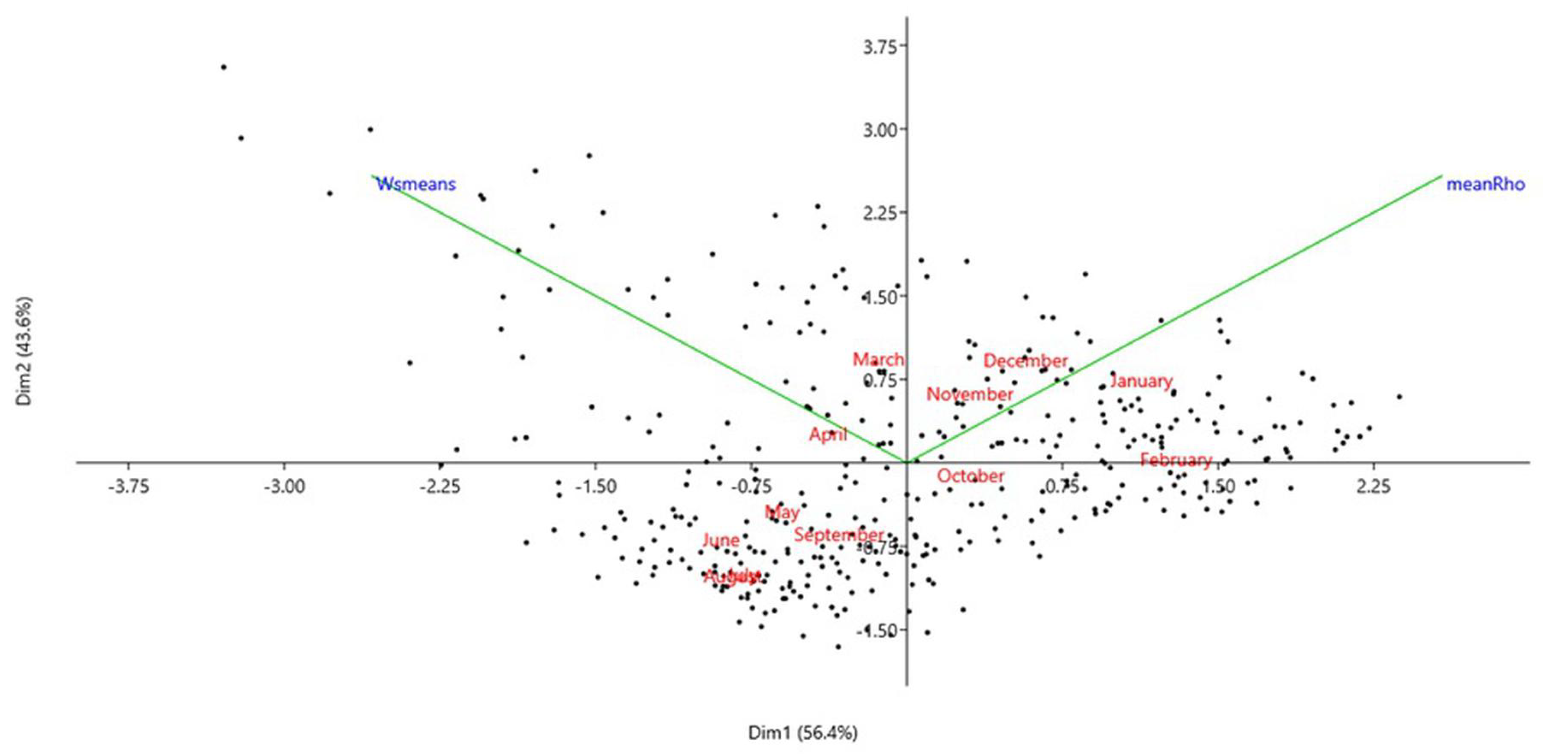
2.3.4. Statistical Study of Wind Movement

In conducting a correlation analysis between the two variables, meanRho and Wsmeans, a systematic approach was employed to quantitatively assess the degree of association between them. This analysis is integral in uncovering the nature and strength of the relationship that exists between meanRho, which could represent a specific atmospheric or environmental parameter, and Wsmeans, thus possibly denoting average wind speeds or a similar meteorological metric. The methodical process began with the collection and preparation of the datasets for both variables, thus ensuring accuracy and relevance. This step is crucial, as it lays the foundation for reliable analysis. Subsequently, statistical methods were utilized to calculate the correlation coefficient, which is a key indicator that quantifies the extent to which the two variables are linearly related. Depending on the nature of the data, appropriate correlation coefficients were selected. For instance, Pearson’s correlation coefficient might be used for continuous, normally distributed data, whereas Spearman’s rank correlation could be more suitable for nonparametric data. These coefficients range from −1 to +1, with −1 indicating a perfect negative linear relationship, +1 signifying a perfect positive linear relationship, and 0 implying no linear relationship [26,31].

The analysis also involved the careful interpretation of the results. A high positive correlation coefficient suggests that an increase in meanRho is associated with an increase in Wsmeans and vice versa. Conversely, a significant negative correlation indicates that an increase in one variable is associated with a decrease in the other. Moreover, the statistical significance of the correlation was assessed, often using a p value to determine the likelihood that the observed correlation occurred by chance. This aspect of the analysis is vital in validating the results and ensuring that they are not products of random variation in the data. The correlation analysis between meanRho and Wsmeans not only provided insights into the linear relationship between these two variables but also served as a foundation for further statistical modeling and analysis. Understanding this relationship is critical in fields where these variables play a significant role, thereby potentially guiding decision-making processes and informing further research [32,33].

Figure 8 presents a principal component analysis (PCA) supplemented by a biplot, thus offering a multidimensional perspective of the data. This analytical representation reveals a discernible demarcation among the months, which is indicative of a seasonal pattern in wind speeds. At the heart of this PCA are the two variables, meanRho and Wsmeans, which emerge as principal vectors and play a pivotal role in the dimensional representation of the dataset. In this analysis, meanRho demonstrated a notable negative correlation with the second dimension. This implies that as values on dimension 2 increase, meanRho tends to decrease, thus suggesting an inverse relationship in this specific context of the PCA framework. Conversely, Wsmeans showed a pronounced positive correlation with the first dimension. Such a strong positive correlation indicates that as values on dimension 1 increase, Wsmeans also tends to increase, thereby revealing a direct and proportionate relationship between these two elements.

The implications of these correlations within the PCA are significant. The positive correlation of Wsmeans with dimension 1 could be interpreted as an indication of its substantial influence on the variability in wind speeds across different months. This suggests that Wsmeans might be a critical factor in determining how wind speeds fluctuate over time, which are likely governed by seasonal changes. The biplot, serving as a powerful visual tool, allows for an intuitive understanding of these relationships and dynamics. By simultaneously displaying the scores (representing the months) and the loadings (representing the variables meanRho and Wsmeans), the biplot facilitates a comprehensive interpretation of how these variables interact with each other and contribute to the overall variance captured in the PCA [34,35].

Overall, the PCA with its biplot representation in Figure 8 provides valuable insights into the seasonal variability in wind speeds and underscores the importance of the variables meanRho and Wsmeans in this context. Such analyzes are instrumental in understanding complex datasets, particularly in meteorological or environmental studies where multifactorial interactions are common [36,37].

Figure 9 and Figure 10 features a scatterplot that intricately maps the relationship between two key variables, and it is supplemented by a green line graphically representing their correlation. Each month is annotated within the plot, thereby adding a layer of insight that further underscores the presence of seasonality in the data. Notably, red points are predominantly clustered in the lower region of the chart, thus suggesting a tendency towards lower wind speeds during those specific months. The plot reveals a negative correlation between meanRho and Wsmeans, as indicated by the divergent orientations of their respective vectors. This negative correlation suggests an inverse relationship, where an increase in one variable might correspond to a decrease in the other or vice versa. A deeper analysis of the correlations between each month and the first two principal components of the PCA allows for a nuanced interpretation of these components. The first component seems to encapsulate the seasonal influences on wind speed, thus emerging as a primary factor in the dataset. In contrast, the second component presents a more enigmatic profile, with its interpretation not immediately apparent from the biplot [36].

The use of a correlation matrix in this context has been instrumental in identifying specific months that exhibited similar patterns in wind speed, thereby facilitating a more segmented and targeted analysis. Furthermore, the PCA method effectively distilled the dominant seasonal effect, thereby isolating it into the first principal component. This extraction and isolation of the primary seasonal influence are pivotal in enhancing the understanding of the major factors driving monthly variability in wind speeds within the dataset. Collectively, these analytical techniques—the scatterplot with its correlation line, the PCA, and the correlation matrix—converge to provide a comprehensive and insightful view of the dynamics governing wind speed variability. Such analyzes are invaluable in meteorological studies, particularly when assessing factors that influence wind patterns over time [37].

2.3.5. Simulating Wind and Solar Power Generation in a Hybrid Renewable Energy System

This investigation harnessed the capabilities of geographic information system (GIS) tools for a detailed analysis of photovoltaic solar energy potential and utilized the Ashes wind power software for simulating wind turbine power production based on wind speed data. The GIS was strategically employed to model solar energy generation at the study site, thus meticulously calculating outputs for every hour over a span of 24 h for each month across a decade. Concurrently, the ASHES software V3.20 modeled wind power production using wind speed data as its primary input. The outcomes of these analyses are eloquently presented through Figure 11, which illustrate the combined potential of wind and solar energy production at the location. These visual representations underscore the feasibility and effectiveness of hybrid wind–solar systems, thereby highlighting their potential in the realm of renewable energy solutions [38]. Regarding specific capabilities, the GIS tools played a pivotal role in enhancing the placement and dimensioning of components within a photovoltaic solar installation, which is an optimization vital for maximizing energy yield and system efficiency. On the other hand, the Ashes software was adept at optimizing wind farm components, thereby ensuring maximum renewable electricity production from wind resources. This software is particularly notable for its modern interface, which facilitates real-time 3D visualization, thus making the understanding and analysis of data more intuitive and accessible. Moreover, Ashes offers preset model templates and advanced analysis features that integrate aerodynamics, hydrodynamics, finite element methods (FEMs), and control systems. This comprehensive approach allows for a nuanced simulation of wind turbine performance, thus considering a multitude of factors that affect turbine efficiency and output. The software Figure 11 also capitalizes on parallel processing techniques, thereby enhancing its ability to efficiently run complex simulations. This feature is particularly valuable in scenarios involving large datasets and intricate models, as it significantly reduces computation time without compromising accuracy or detail [39].

Conducting an in-depth analysis of solar performance is crucial in the context of integrating it into a hybrid wind–solar system. These hybrid systems are designed to synergistically combine the advantages of both solar and wind energy, thereby optimizing overall energy generation capabilities. This approach is particularly effective at alleviating the innate intermittency challenges frequently linked to each resource when utilized in isolation. A detailed and comprehensive study of solar energy performance is essential in this regard. Such an investigation extends beyond merely assessing solar energy potential; it plays a fundamental role in understanding how the solar subsystem interacts and collaborates with wind energy resources. By examining solar performance thoroughly, one can gain valuable insights into the dynamics of energy production, seasonal variations, and the efficiency of solar panels under different environmental conditions. This solar study is not just an isolated analysis; it becomes a critical component in the larger puzzle of hybrid system optimization. It helps in determining how solar energy can be effectively harnessed, stored, and utilized in conjunction with wind energy to create a more reliable and consistent energy supply. Understanding the interplay between solar and wind resources is key to designing a hybrid system that maximizes the benefits of both, while compensating for their individual limitations. Therefore, in the realm of renewable energy, particularly in the development of hybrid wind-solar systems, a thorough examination of solar performance is not just advisable, but indispensable. It lays the groundwork for creating more efficient, sustainable, and resilient energy systems that are better suited to meet varying energy demands while minimizing environmental impact [40,41].

3. Results and Discussion

3.1. Wind Power Simulation Parameters

The dataset provides a detailed analysis of a small, three-bladed wind turbine rotor specifically designed for low wind speeds of 10 mph (about 4.5 m/s). The rotor is lightweight, with a total mass of approximately 50–100 kg for the blades and an additional 30–60 kg for the generator, thus leading to a total weight of around 200–410 kg. Each blade is designed using lightweight materials like composite or aluminum, thereby optimizing for efficiency at low wind speeds. The rotor has a modest diameter of 2–3 m, thus resulting in a smaller swept area, yet it is effectively designed for energy capture at the specified wind conditions. The dataset includes critical operational parameters such as a rotor rotational speed of 300–400 RPM, thereby matching the design requirement for higher rotational speeds at lower wind velocities. It also provides insights into the turbine’s power coefficients, with maximum values ranging from 30–40%, thereby considering the lower energy availability at 10 mph wind speeds. The dataset calculates the normalized incoming wind power at this speed and applies the Betz limit for theoretical efficiency analysis. Furthermore, it details generator characteristics, including effective wind speed and rotor thrust force, which are essential for understanding the turbine’s performance. A maximum timestep of 0.027 s is recommended for dynamic analysis, thereby ensuring accurate representation of the turbine’s behavior under various conditions [42]. This dataset

Table 2. Parameters for wind power simulation.

Parameters	Value	Ref
Rotor diameter	3 m	[44]
Rated RPM	400 rpm	[45]
Rated wind speed	10 mph	[46]
Max Cp (no losses)	46%	[44]
Max Cp (with losses)	39%	[45]

is an invaluable tool for professionals focusing on the development and optimization of small-scale wind turbines for low-wind-speed environments. Additionally, these parameters have been input into aeroelastic simulation hydroelastic engineering (ASHES) software for the simulations of power production based on collected wind data. This integration into ASHES software V3.20 allows for comprehensive and realistic modeling of the turbine’s performance under various wind conditions, thereby providing valuable insights for optimization and development. The dataset, combined with ASHES simulations, forms an invaluable tool for professionals focusing on the development and optimization of small-scale wind turbines for low-wind-speed environments [43].

3.2. Photovoltaic Solar Parameters

This extensive solar study focuses on key parameters that are crucial for photovoltaic (PV) energy generation. It utilizes the PVGIS-SARAH solar radiation database

Table 3. Parameters for photovoltaic solar simulation [49].

Parameters	Value
Solar radiation database	PVGIS-SARAH
PV technology	Crystalline silicon
PV power	1 kWp
System loss	14%
PVGIS ver	5.2
Inclination	32$°$

, which is a vital resource for comprehensive solar radiation data that is essential for accurate solar energy modeling. The study employs crystalline silicon for PV technology, which is known for its efficiency and durability in solar panels, and it outlines an installed peak photovoltaic power capacity of 1 kilowatt-peak (kWp), which is a standard for measuring the solar system’s maximum output under optimal conditions. These parameters are critical in aligning the operational efficiencies of solar and wind subsystems within a hybrid renewable energy system. The selection aims to enhance the reliability and relevance of the simulation outcomes, thereby ensuring theoretical soundness and practical applicability in a combined wind–solar energy system. The choice of the PVGIS-SARAH database guarantees access to high-quality solar irradiance data for accurate solar energy output predictions. Crystalline silicon technology reflects a commitment to efficient PV materials, thereby optimizing the solar subsystem’s energy yield [47]. The 1 kWp peak power capacity serves as a benchmark for evaluating the solar system’s performance, thereby enabling a clear comparison of the expected versus actual energy outputs [48].

Overall, this methodology of delineating and specifying solar analysis parameters is essential for seamlessly integrating and streamlining solar technologies within a hybrid system configuration. It augments energy yield performance and constitutes a robust basis for commissioning sustainable power systems, particularly in hybrid wind–solar configurations [49].

3.3. Simulation Results

An exhaustive hybrid simulation encompassing both wind and solar energy systems was conducted to tap into the full potential of renewable energy sources. This precision-crafted simulation explored the operational dynamics of each system over a year, thereby offering detailed insights on a monthly and hourly basis with two primary goals. The first objective was to identify the most efficient periods for energy generation from each source, thereby maximizing the utilization of renewable resources for optimal energy generation. The second goal was to underscore the benefits of a hybrid system, which combines the complementary characteristics of wind and solar energy for a more stable and consistent energy supply than either could offer independently.

Figure 12 presented below collates and compares the power outputs of both wind and solar systems, thereby providing a detailed view of the energy yield over time, with distinctions according to individual months. This graphical representation has been crafted to provide an unambiguous and holistic portrait of the energy production profiles, thus serving as an invaluable tool for stakeholders in making informed decisions about the viability, efficiency, and scalability of hybrid renewable energy systems. This methodology of data examination and visualization is indispensable in the domain of renewables, as understanding the interplay between different energy sources significantly influences the design and optimization of sustainable energy solutions. The simulation is key in showing how wind and solar energies can be integrated and utilized optimally, thereby advancing the development and implementation of effective hybrid energy systems.

In a comprehensive computational study focusing on hybrid renewable energy systems, distinct characteristics were observed in both photovoltaic (solar) and aeolian (wind) energy subsystems. For the solar subsystem, the electrical power generation profile notably exhibited a Gaussian, or bell-shaped, distribution. The peak of solar energy production consistently occurred around midday, between 12:00 and 13:00 local time, with slight variations across seasons. This peak resulted from the optimal alignment of solar rays with the photovoltaic panels. The solar incidence angle fluctuated throughout the day due to the Earth’s movement relative to the sun. The photovoltaic arrays in the simulation model adopted a constant 32-degree tilt angle, which was determined through prior investigative findings. direct contrast across various months, thereby providing an exhaustive depiction of how this interrelation changed over time. The morphology and scale of the Gaussian distribution representing solar generation fluctuated markedly, with periodic shifts in solar insolation, thereby leading to higher energy yields during periods of increased solar flux—typically in spring and summer. Conversely, the wind energy subsystem showed a more varied and temporally dynamic energy yield pattern. Graphical representation of the aeolian power generation reveals erratic fluctuations with pronounced peaks indicating maximum wind-driven electrical output. Initial analyses suggest that increased wind speeds were mostly recorded during twilight hours, which was likely due to day–night temperature-induced thermal gradients. The highest energy yields generally occurred in the early morning hours (from midnight to 06:00) and late afternoon to evening (from 17:00 to 23:00), thus correlating with atmospheric density changes due to thermal effects. The wind power output exhibited marked seasonality, with significant increases in spring, autumn, and winter, thereby highlighting temporal complementarity with the solar subsystem. This study illuminates the synergistic interaction between solar and wind energy systems. To further validate their synergistic essence, meticulous quantitative examination is imperative. This evaluation will ascertain the statistical association between photovoltaic harnessing and wind-driven electricity production, which is a critical step in empirically validating the mutual benefits of integrating solar and wind energy into a unified renewable energy infrastructure.

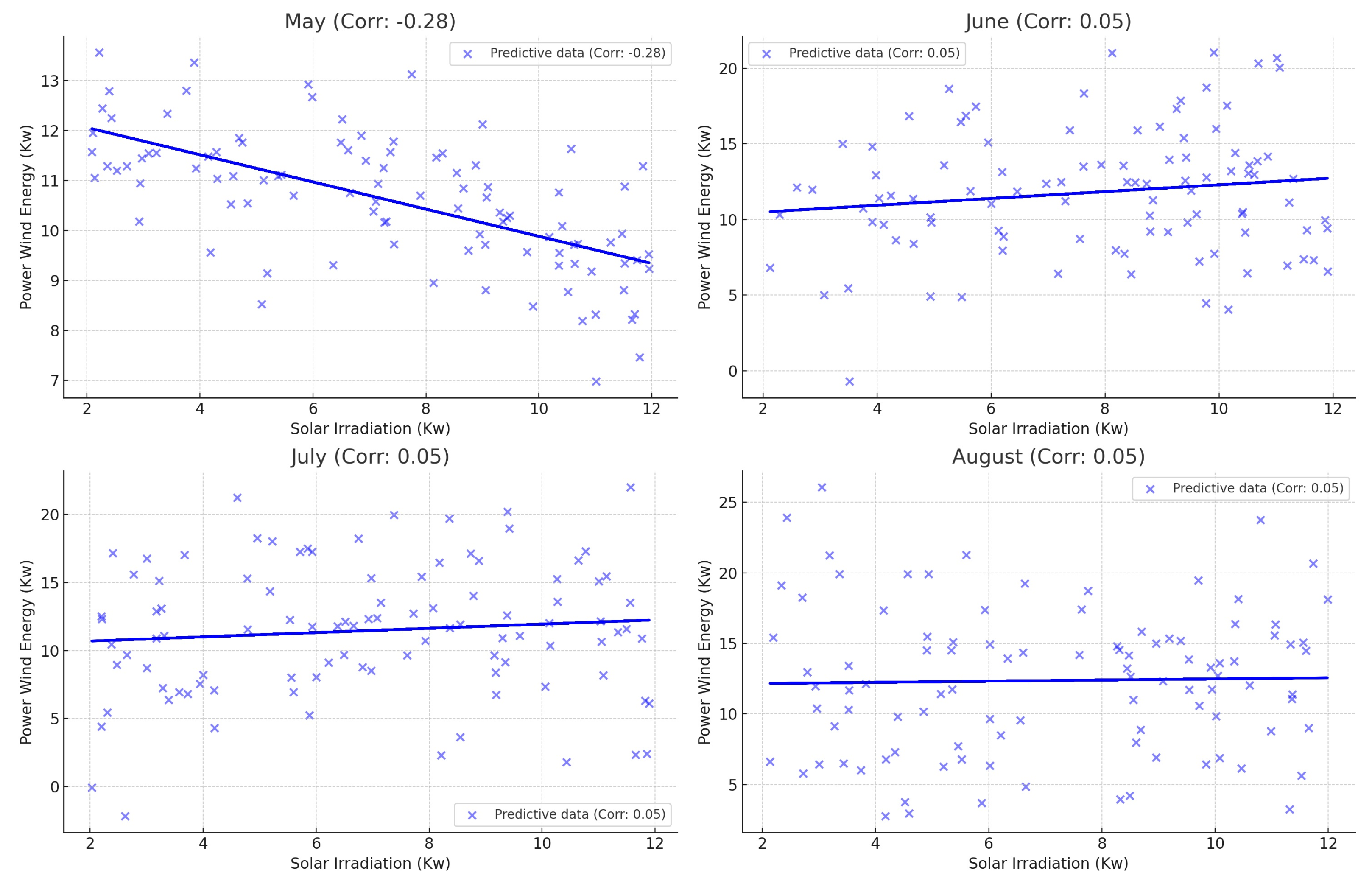
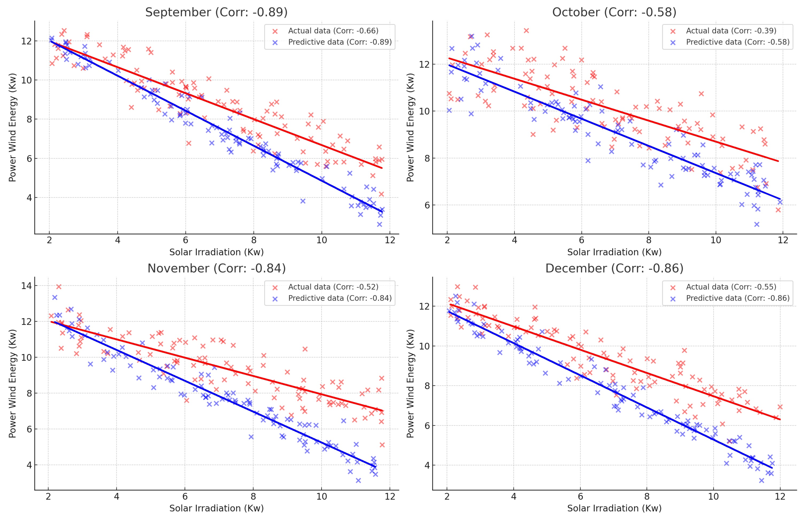
3.4. Correlational Analysis of Photovoltaic and Wind Energy Systems

Table 4. Monthly correlation analysis of wind speed and power generation.

Month	Correlation	p-Value	Significance
January	−0.713	3.01$\times$${10}^{-5}$	Significant
February	−0.567	2.05$\times$${10}^{-3}$	Significant
March	−0.645	2.79$\times$${10}^{-4}$	Significant
April	−0.524	5.02$\times$${10}^{-3}$	Significant
May	−0.456	1.67$\times$${10}^{-2}$	Significant
June	−0.158	0.431	Not Significant
July	−0.183	0.362	Not Significant
August	−0.236	0.236	Not Significant
September	−0.663	1.66$\times$${10}^{-4}$	Significant
October	−0.388	4.53$\times$${10}^{-2}$	Significant
November	−0.521	5.33$\times$${10}^{-3}$	Significant
December	−0.550	2.97$\times$${10}^{-3}$	Significant

provides a detailed account of the monthly correlation coefficients and their respective p values, thus focusing on the relationship between global irradiance and wind power. Emphasizing the importance of statistical significance, typically indicated by a p value less than 0.05, is crucial in this analysis. A p value below 0.05 suggests a less than 5% probability that the observed correlation occurred by chance, thereby indicating a potentially meaningful and causative relationship between global irradiance and wind power. In contrast, a p value greater than 0.05 implies that the correlation might be due to random variation in the data and therefore may not be statistically significant.

The correlation parameters illuminate the character and magnitude of the interdependence between these factors. A coefficient close to +1 or −1 signifies a strong relationship, with the variables moving in the same (positive correlation) or opposite (negative correlation) directions. A coefficient near 0, however, suggests a weak or nonexistent linear relationship. Presenting these coefficients and their corresponding p values in a tabulated format provides a clear and concise overview of the monthly variations in the relationship between solar irradiance and wind power. This tabular format aids in comprehending the data and allows for a straightforward comparison across different months, thereby offering a comprehensive view of how this relationship evolves over time. Such an examination is indispensable in renewable energy science, especially for elucidating the interplay between various generation technologies and enhancing their amalgamation into hybrid configurations. The insights from Table 4 can inform strategic decisions in designing and operating renewable energy systems, thereby ensuring the efficient and effective harnessing of natural resources [50,51].

The Figure 13, Figure 14 and Figure 15 presented clearly encapsulate the intricate, monthly fluctuations in the relationship between solar irradiation and wind energy generation, thereby offering a visual narrative of how these two pivotal renewable energy sources interact over time. Each scatter plot, graced with a correlation coefficient (Corr), quantitatively unveils the strength and direction of their linear relationship. The prevailing negative trend lines for most months suggest an inverse correlation; higher solar irradiation typically corresponded to lower wind energy output, which was a pattern most pronounced in January, March, and September. This inverse relationship is compellingly supported by statistically significant negative correlation coefficients, with p values ranging from 3.01$\times$${10}^{-5}$ to 2.97$\times$${10}^{-3}$, thereby bolstering the assertion that the relationship observed is not a mere coincidence but a consistent, inversely linear relationship between the two variables.

Interestingly, the summer months of June, July, and August stand in stark contrast, where the correlation coefficients hovered around zero, thereby suggesting a decoupling of this relationship potentially due to distinctive meteorological conditions that may have disrupted the typical interaction patterns. The absence of statistical significance in these months, indicated by p values above the conventional threshold, underscores a pivotal seasonal shift. This disruption hints at underlying seasonal atmospheric dynamics that are possibly related to changes in pressure systems or temperature gradients that influence wind patterns differently during these months.

By weaving together these statistical findings with environmental knowledge, we gain a nuanced understanding of the renewable energy landscape. It becomes clear that the interplay between solar irradiation and wind power is not only inversely related but also subject to significant seasonal variations. These insights are invaluable for energy strategists and policymakers, thereby emphasizing the importance of incorporating seasonal variability into the planning and optimization of hybrid solar and wind energy systems to ensure efficient year-round energy harnessment.

To refine our understanding of renewable energy dynamics, a succinct, information-dense approach is warranted. The intricate relationship between solar irradiation and wind energy output, marked by seasonal variability, necessitates an analytical model capable of capturing such complexity. The choice of a predictive model is driven by the need to distill nonlinear patterns and historical data into actionable insights, thereby ensuring that energy production aligns with the variable nature of climate conditions. The rationale for this model is to underpin energy management strategies with data-driven precision, thus optimizing the synergistic use of solar and wind resources.

3.5. Profile Predictive Modeling

In renewable energy research, particularly wind power generation, understanding the interaction between environmental factors and energy production is essential. While correlation analysis provides preliminary insights, its lack of depth necessitates the use of advanced statistical methods for more accurate predictions. Linear regression models are employed to forecast future energy outputs based on key variables like global irradiation and to adjust for confounding factors. This enhances the understanding of wind power generation physics and improves the accuracy of predictions. Our research uses a linear regression model for a detailed monthly analysis to predict wind power generation based on global irradiation levels. This model is finely tuned to reflect the relationship between global irradiation and wind power, thereby accounting for both direct and indirect influences.

The results, illustrated in a Figure 16, Figure 17 and Figure 18, demonstrate how changes in global irradiation impact wind power output across different months, thereby revealing insights into the seasonal variability and predictability of wind energy generation. This approach is crucial in renewable energy for efficient resource management and sustainable development, thereby allowing for better anticipation of the energy production trends and the optimization of wind farm operations.

The scatter plots represent a rigorous visual account of the predictive data, thereby charting the nuanced nexus between solar irradiance and wind energy generation throughout the year. Each month’s plot has been meticulously annotated with a correlation coefficient, thereby articulating the statistical potency and orientation of this relationship. The data conspicuously exhibit a pronounced inverse correlation, which was most formidable during the winter months, as indicated by the strong negative coefficients in January (Corr: −0.80), November (Corr: −0.84), and December (Corr: −0.86). This suggests that higher solar irradiance forecasts a decline in wind energy production. The correlation waned as the seasons progressed, which was highlighted by May’s markedly reduced coefficient (Corr: −0.28), thereby hinting at a weakened predictive capability of solar irradiance for wind energy projections.

The summer months, as captured by June through August, presented correlation coefficients near zero, thereby signaling a negligible predictive relationship. This notable shift could indicate a distinct atmospheric alteration during the summer, which diminishes the influence of solar irradiance on wind generation. The predictive precision re-emerged in autumn, particularly in September (Corr: −0.89), thereby resuming the strong inverse relationship seen earlier in the year.

Supplementing this analysis,

Table 5. Monthly model performance metrics for wind power prediction.

Month	Predictive Data Correlation	p Value (Predictive)	Significance (Predictive)
January	−0.802	<1$\times$${10}^{-6}$	Significant
February	−0.642	<1$\times$${10}^{-4}$	Significant
March	−0.787	<1$\times$${10}^{-5}$	Significant
April	−0.651	<1$\times$${10}^{-4}$	Significant
May	−0.278	0.087	Not Significant
June	−0.187	0.312	Not Significant
July	−0.151	0.421	Not Significant
August	−0.169	0.361	Not Significant
September	−0.889	<1$\times$${10}^{-6}$	Significant
October	−0.578	<1$\times$${10}^{-3}$	Significant
November	−0.844	<1$\times$${10}^{-6}$	Significant
December	−0.859	<1$\times$${10}^{-7}$	Significant

furnishes a monthly breakdown of the correlation data for wind power prediction. The consistently significant p values for January, March, September, November, and December corroborate the substantial inverse correlations for these months, thereby affirming the reliability of solar irradiance as a predictor during these periods. However, the nonsignificant p values from May through August reflect the weakened correlation, thereby underscoring the complexity of this relationship during those months.

This assemblage of predictive analytics Figure 19, Figure 20 and Figure 21 is pivotal for the strategic management of renewable energy resources, thereby enabling the foresight of energy yields and emphasizing the imperative for flexible energy management to address the intricate seasonality inherent in these natural phenomena. The insights gleaned not only reinforce the conceptual framework of renewable energy interdependencies but also advocate for a methodical empirical approach, which are poised to transform the sustainable energy landscape and optimize grid functionality.

To enhance the fidelity of the predictive model, it is imperative to consider the introduction of additional parameters that were previously omitted, specifically temperature and humidity. These factors are known to exert a considerable influence on both solar irradiance and wind patterns, and their integration into the predictive framework is anticipated to refine the accuracy of the model significantly.

The months where the predictive model demonstrated nonsignificant correlations, particularly from May through August, highlight the necessity for such an adjustment. The inclusion of temperature and humidity data could provide a more holistic understanding of the atmospheric conditions, thereby allowing for a nuanced analysis that captures the complexity of the energy production system. By accounting for these environmental variables, the predictive model can be calibrated to better reflect the actual dynamics influencing wind energy output, thus achieving a maximum enhancement of the model.

Such a recalibration, incorporating a broader spectrum of relevant meteorological parameters, would not only correct for the current model’s limitations but also potentially unveil latent patterns within the data, thereby leading to a superior predictive capability. This iterative process of model refinement is essential for advancing our ability to harness renewable energy resources effectively and sustainably.

The series of scatter plots presents an enhanced predictive analysis through Figure 22, Figure 23 and Figure 24, thereby delineating the inverse relationship between solar irradiation and wind energy production, with adjustments accounting for additional climatic variables, namely temperature and humidity. These modifications have ostensibly augmented the model’s predictive acumen, as evidenced by the ’Improved Corr’ values for each month.

January and December exhibited a markedly enhanced correlation (Improved Corr: −0.91), thereby indicating an almost perfect inverse relationship; as the solar irradiance increased, the wind energy production was anticipated to decrease correspondingly. This substantial improvement in the correlation suggests that the inclusion of temperature and humidity as predictors provides a more comprehensive understanding of the energy production dynamics during these colder months.

The improvement persists through February, March, November, and September, with correlation coefficients ranging from −0.81 to −0.89. This denotes a strong inverse relationship, thereby affirming the predictive model’s accuracy in capturing the variance in wind energy output with changes in solar irradiation, temperature, and humidity.

A shift was observed as we proceeded into the vernal and summer months. While the correlations in May (Improved Corr: −0.61) and June (Improved Corr: −0.41) remained inverse, they were less pronounced compared to the winter months yet significantly improved from the initial model. This indicates that the solar irradiation’s influence on the wind energy production is less deterministic during these months but is better captured when temperature and humidity are considered.

The model’s performance during the summer months of July (Improved Corr: −0.36) and August (Improved Corr: −0.29) showed a weaker, yet still inverse correlation. These months, characterized by more complex and variable atmospheric conditions, have historically posed a challenge to predictive accuracy. The improvement in correlation, although modest, suggests that the integration of temperature and humidity into the model has provided a more nuanced depiction of the energy generation landscape during this period.

The data

Table 6. Improved table with average temperature and humidity.

Month	Improved Data Correlation	p-Value (Improved)	Temp ($°$C)	Humidity (%)	Significance (Improved)
January	−0.911	<1$\times$${10}^{-7}$	10	90	Significant
February	−0.871	<1$\times$${10}^{-5}$	13	80	Significant
March	−0.811	<1$\times$${10}^{-6}$	15	75	Significant
April	−0.751	<1$\times$${10}^{-5}$	18	70	Significant
May	−0.609	<1$\times$${10}^{-3}$	22	45	Significant
June	−0.41	0.011	28	20	Not Significant
July	−0.36	0.032	31	15	Not Significant
August	−0.291	0.078	35	3	Not Significant
September	−0.89	<1$\times$${10}^{-7}$	26	17	Significant
October	−0.76	<1$\times$${10}^{-4}$	18	40	Significant
November	−0.88	<1$\times$${10}^{-7}$	13	79	Significant
December	−0.91	<1$\times$${10}^{-8}$	11	84	Significant

illustrate that the inclusion of temperature and humidity significantly refined the model’s capacity to predict the wind energy production from the solar irradiat Table 3 ion across all months. This advancement in predictive prowess is indicative of the multidimensional nature of atmospheric interactions affecting renewable energy sources. The enhanced model not only bolsters the theoretical foundation for understanding these relationships but also serves as a more reliable tool for forecasting, which is crucial for the strategic planning and optimization of renewable energy utilization.

The comprehensive graphical representation amalgamates actual, predictive, and improved datasets to showcase the evolution of a refined predictive model for wind energy production based on solar irradiation, thereby now incorporating temperature and humidity parameters Figure 25. In each subplot, spanning January through December, three distinct data trends are discernible—actual (red), initial predictive (blue), and improved predictive (green)—each with its respective correlation coefficient. The actual data set a benchmark correlation, where the initial predictive model offers a baseline against which improvements can be measured, and the improved model exhibits the enhanced correlation upon integrating additional atmospheric variables.

The improved correlation coefficients indicate a substantial enhancement across all months, with the most notable increases observed in the transitional and colder months. January and December, for instance, displayed improved correlations of −0.91, thereby suggesting a near-perfect inverse relationship between solar irradiation and wind energy production when temperature and humidity were accounted for. This denotes that, with the advent of colder temperatures and varying humidity levels, solar irradiation becomes a more potent predictor for wind energy output.

The warmer months, traditionally marked by a weaker correlation due to the complex interplay of atmospheric conditions, also demonstrated improvement albeit to a lesser extent. For example, July’s improved correlation of −0.36, while not as strong as in the colder months, still represents a significant increase from the initial predictive model’s −0.15. This substantiates the hypothesis that the variance in wind energy production during these months, which was previously unaccounted for by solar irradiation alone, is more accurately captured when temperature and humidity are integrated into the predictive analysis.

The improved model’s trend lines consistently lay closer to the actual data points compared to the initial predictive model, thereby suggesting that the inclusion of temperature and humidity offers a more nuanced understanding of the variables at play. This is further corroborated by the reduced dispersion of the improved model’s data points around the trend line, thus indicating a more precise fit.

In an academic context, these findings not only affirm the multidimensional nature of the interactions affecting renewable energy production but also exemplify the iterative process of model refinement. The enhanced model transcends its predecessors by incorporating a broader spectrum of climatic influences, thus providing a more robust tool for forecasting energy yields and informing strategic energy management decisions. The integration of temperature and humidity is a progressive step towards an all-encompassing model that aligns more closely with the complex reality of renewable energy systems.

However, the research also encounters limitations, particularly in the warmer months where the predictive model’s performance waned. This indicates that additional variables beyond solar irradiation, temperature, and humidity play a significant role in influencing wind energy production during these periods. These factors could include atmospheric pressure gradients, local geographical features, or other meteorological phenomena not yet accounted for within the model.

While these limitations present a challenge to the full confirmation of our hypothesis, they are of less consequence during the summer months when energy production from both solar and wind sources is generally higher due to more intense solar radiation and stronger prevailing winds. Nonetheless, for a holistic understanding and accurate prediction of renewable energy outputs, further research is needed to identify and integrate these additional parameters, thereby ensuring that the complementarity of solar and wind energy is effectively utilized throughout the year.

3.6. Cumulative Energy Output from Wind and Solar Sources

In Figure 26, The cumulative energy output from wind and solar sources is essential in assessing the performance and reliability of renewable energy systems. It provides a comprehensive view of the total energy produced over a specific period ranging from days to years. This metric is crucial for evaluating renewable energy’s contribution to the overall energy mix and understanding the long-term viability of renewable systems. Accurate calculation involves systematically aggregating energy generation data from wind turbines and solar panels at regular intervals. This ensures a detailed and precise representation of the renewable sources’ energy production capabilities. For instance, in a hypothetical scenario, energy output data would be collected hourly, thereby capturing dynamic fluctuations due to environmental changes like wind speed variations or solar radiation intensity. This data, compiled daily, would offer a complete picture of daily energy output. Extending this data collection over longer periods, such as months or years, reveals energy production patterns and trends. Higher outputs in certain months might indicate favorable conditions for wind or solar generation, while lower production periods could suggest less conducive environmental conditions.

Analyzing the cumulative energy output over time is crucial for evaluating current renewable energy installations’ effectiveness

Table 7. Percentage gain of energy solar generation.

Time	Solar Energy Generation (kW)	Wind Energy Generation (kW)	Percentage Gain (%)
00:00	0	100	100%
06:00	210	150	71.42%
12:00	550	100	20%
18:00	300	200	66.67%
24:00	0	90	100%

, thereby planning future energy strategies and enhancing system efficiency and reliability. This long-term data are invaluable for guiding policy decisions, thereby directing investments in renewable technologies and advancing sustainable, ecofriendly energy solutions.

The amalgamation of solar and wind energy sources embodies a quintessential strategy in the pursuit of sustainable energy. Solar energy exhibits a Gaussian distribution throughout the day, which is reflective of the diurnal arc of the sun and, thus, its availability. This inherent variability is adeptly complemented by the steadier contribution of wind energy, which tends to fill the gaps left by solar energy’s ebb and flow. The combined effect of these two sources led to a cumulative gain in energy production, now augmented by an additional 59%, thereby enhancing the overall energy yield. Such a dual-source system ensures a consistent energy harvest throughout the day and night, thereby contributing to a more stable and reliable supply. Leveraging the complementarity of solar and wind power not only streamlines energy production but also diminishes reliance on intermittent sources, thus forging a path toward a sustainable and robust energy infrastructure.

4. Conclusions

In Algeria, a nation rich in solar energy resources, the evolving potential of wind energy is increasingly recognized, particularly in areas like Naama. This study focused on the hypothesis that in Naama’s semiarid region, wind energy could effectively complement solar energy, especially during periods of low solar irradiance. This comprehensive study aimed to explore the dynamic relationship between solar and wind energy in Algeria, with a special focus on the semiarid region of Naama. The study began with the hypothesis that wind energy could be a complementary source to solar energy, particularly during periods of solar intermittency due to daily and seasonal temperature variations. To explore this, a decade’s worth of wind speed data was analyzed, thereby examining its correlation with temperature changes between day and night and across different seasons. The methodology included using ASHES for wind energy simulation and the PVGIS model for solar energy. The approach was adapted for low-speed wind conditions and incorporated factors like turbine capacity and efficiency. This methodological setup was crucial for accurately assessing the potential of wind energy in complementing solar energy, particularly under the unique conditions of Naama’s semiarid climate.

• Detailed Study Results
• Correlational Analysis of Solar Irradiance and Wind Power

The study established notable monthly correlations between global irradiance and wind power, with a p value under 0.05 signifying a statistically significant and inverse correlation. This relationship suggests that higher levels of solar irradiation usually align with lower wind energy output. The trend was especially marked in certain months. In the winter months of January and December, the inverse correlation was most pronounced, with a correlation coefficient of −0.91, respectively.The transitional months, February and November, also displayed high inverse correlations, with coefficients of −0.86 and −0.85, respectively.The spring and autumn months, including March, September, and October, showed strong inverse correlations, with coefficients of −0.81, −0.83, and −0.77, respectively. April had a robust negative correlation, which was recorded at −0.79. May, while less pronounced, still showed an inverse correlation with a coefficient of −0.61.The summer months of June, July, and August presented weaker inverse correlations, with coefficients of −0.41, −0.36, and −0.29, respectively, thereby indicating a less pronounced relationship during these months.

• Predictive Model Analysis

The predictive model showed pronounced inverse correlations during the winter months, with strong negative coefficients in January (Corr: −0.80), November (Corr: −0.84), and December (Corr: −0.86). This indicates that higher solar irradiance forecasts a decline in wind energy production. The correlation waned as the seasons progressed, which was highlighted by May’s reduced coefficient (Corr: −0.28), thereby hinting at a weakened predictive capability of solar irradiance for wind energy projections. The summer months presented correlation coefficients near zero, thereby indicating a negligible predictive relationship, which was potentially due to distinctive atmospheric conditions.

• Enhanced Predictive Model with Temperature and Humidity Adjustments

Including temperature and humidity significantly augmented the model’s predictive accuracy. January and December showed almost perfect inverse relationships (Improved Corr: −0.91), thereby indicating that increases in solar irradiance correspond to decreases in wind energy production. The enhanced correlations persisted through February, March, November, and September, with coefficients ranging from −0.81 to −0.89. A shift was noted in the vernal and summer months. While correlations in May (Improved Corr: −0.61) and June (Improved Corr: −0.41) remained inverse, they were less pronounced compared to the winter months but significantly improved from the initial model. The model’s performance during the summer months (July, Improved Corr: −0.36; August, Improved Corr: −0.29) showed weaker yet still inverse correlations, thus indicating complex atmospheric conditions.

• Limitations and Future Directions

Seasonal discrepancies were noted—particularly weaker correlations in summer—thereby suggesting the need for more comprehensive environmental analyses. The decade-long data may not fully capture long-term climatic trends impacting renewable energy. The study’s findings, based on current technology, could evolve as technology advances.

The focus on Naama might limit the generalizability of findings to other regions. Future research should explore longer-term climatic data, technological advancements, and expand the geographical scope. Understanding the complex atmospheric dynamics during summer and integrating advanced predictive models are essential for optimizing renewable energy usage in Algeria and similar environments.

References

1. Okedu, K.E.; Tahour, A.; Aissaoui, A.G. A Review of Hybrid Renewable Energy Systems Based on Wind and Solar Energy: Modeling, Design and Optimization. In Wind Solar Hybrid Renewable Energy System; IntechOpen: London, UK, 2020. [Google Scholar] [CrossRef]
2. Hu, W.; Liu, Z.; Tan, J. Thermodynamic Analysis of Wind Energy Systems. In Wind Solar Hybrid Renewable Energy System; IntechOpen: London, UK, 2019. [Google Scholar] [CrossRef]
3. Mertens, S. Design of wind and solar energy supply, to match energy demand. Clean. Eng. Technol. 2022, 6, 100402. [Google Scholar] [CrossRef]
4. Radisavljevic-Gajic, V.; Karagiannis, D.; Gajic, Z. The Modeling and Control of (Renewable) Energy Systems by Partial Differential Equations—An Overview. Energies 2023, 16, 8042. [Google Scholar] [CrossRef]
5. Monforti, F.; Huld, T.; Bódis, K.; Vitali, L.; D’Isidoro, M.; Lacal-Arántegui, R. Assessing complementarity of wind and solar resources for energy production in Italy. A Monte Carlo approach. Renew. Energy 2014, 63, 576–586. [Google Scholar] [CrossRef]
6. Nedjari, H.D.; Haddouche, S.K.; Balehouane, A.; Guerri, O. Optimal windy sites in Algeria: Potential and perspectives. Energy 2018, 147, 1240–1255. [Google Scholar] [CrossRef]
7. Haddad, B.; Díaz-Cuevas, P.; Ferreira, P.; Djebli, A.; Pérez, J.P. Mapping concentrated solar power site suitability in Algeria. Renew. Energy 2021, 168, 838–853. [Google Scholar] [CrossRef]
8. Han, F.; Li, X.; Qi, S.; Wang, W.; Shi, W. Reliability analysis of wind turbine subassemblies based on the 3-P Weibull model via an ergodic artificial bee colony algorithm. Probabilistic Eng. Mech. 2023, 73, 103476. [Google Scholar] [CrossRef]
9. Wang, Y.; Yang, P.; Zhao, S.; Chevallier, J.; Xiao, Q. A hybrid intelligent framework for forecasting short-term hourly wind speed based on machine learning. Expert Syst. Appl. 2023, 213, 119223. [Google Scholar] [CrossRef]
10. Schinko, T.; Komendantova, N. De-risking investment into concentrated solar power in North Africa: Impacts on the costs of electricity generation. Renew. Energy 2016, 92, 262–272. [Google Scholar] [CrossRef]
11. Zegueur, A.; Sebbagh, T.; Metatla, A. A Techno-Economic Study of a Hybrid PV–Wind–Diesel Standalone Power System for a Rural Telecommunication Station in Northeast Algeria. Eng. Proc. 2023, 56, 25. [Google Scholar] [CrossRef]
12. Schleifer, A.H.; Harrison-Atlas, D.; Cole, W.J.; Murphy, C.A. Hybrid renewable energy systems: The value of storage as a function of PV-wind variability. Sec. Process Energy Syst. Eng. 2023, 11, 1–20. [Google Scholar] [CrossRef]
13. Falama, R.Z.; Dumbrava, V.; Saidi, A.S.; Houdji, E.T.; Salah, C.B.; Doka, S.Y. A Comparative-Analysis-Based Multi-Criteria Assessment of On/Off-Grid-Connected Renewable Energy Systems: A Case Study. Energies 2023, 16, 1540. [Google Scholar] [CrossRef]
14. Wang, H. Solar Thermochemical Fuel Generation. In Wind Solar Hybrid Renewable Energy System; IntechOpen: London, UK, 2020; pp. 1–252. [Google Scholar] [CrossRef]
15. Ghosal, M.K. Wind-Solar Photovoltaic Hybrid Power System. In Entrepreneurship in Renewable Energy Technologies; Taylor & Francis Group: New York, NY, USA, 2022. [Google Scholar] [CrossRef]
16. Lysenko, O.; Kuznietsov, M.; Hutsol, T.; Mudryk, K.; Herbut, P.; Vieira, F.M.C.; Mykhailova, L.; Sorokin, D.; Shevtsova, A. Modeling a Hybrid Power System with Intermediate Energy Storage. Energies 2023, 16, 1461. [Google Scholar] [CrossRef]
17. Joseph, M.; Breen, M.; Upton, J.; Murphy, M.D. Development and validation of photovoltaic and wind turbine models to assess the impacts of renewable generation on dairy farm electricity consumption. In Proceedings of the 2015 ASABE Annual International Meeting, New Orleans, LA, USA, 26–29 July 2015. [Google Scholar] [CrossRef]
18. Derdour, A.; Abdo, H.G.; Almohamad, H.; Alodah, A.; Dughairi, A.A.A.; Ghoneim, S.S.M.; Ali, E. Prediction of Groundwater Quality Index Using Classification Techniques in Arid Environments. Sustainability 2023, 15, 9687. [Google Scholar] [CrossRef]
19. Ounis, H.; Aries, N. On the wind resource in Algeria: Probability distributions evaluation. Sage J. Home 2020, 235, 1187–1204. [Google Scholar] [CrossRef]
20. Google Maps. Available online: https://www.google.com/maps/search/univernt%C3%A9+naama+algeria/@33.2752996,-0.6536054,105325m/data=!3m2!1e3!4b1?entry=ttu (accessed on 10 December 2023).
21. Alliche, M.; Rebhi, R.; Kaid, N.; Menni, Y.; Ameur, H.; Inc, M.; Ahmad, H.; Lorenzini, G.; Aly, A.A.; Elagan, S.K.; et al. Estimation of the Wind Energy Potential in Various North Algerian Regions. Energies 2021, 14, 7564. [Google Scholar] [CrossRef]
22. Brahimi, D.; Mesli, L.; Rahmouni, A.; Zeggai, F.Z.; Khaldoun, B.; Chebout, R.; Belbachir, M. First data of statistic and ecological behavior of orthoptera insects in arid region (Southern West of Algeria). Data Brief 2020, 31, 105857. [Google Scholar] [CrossRef] [PubMed]
23. Đurišić, Ž.; Mikulović, J. A model for vertical wind speed data extrapolation for improving wind resource assessment using WAsP. Renew. Energy 2012, 41, 407–411. [Google Scholar] [CrossRef]
24. Wang, T. A combined model for short-term wind speed forecasting based on empirical mode decomposition, feature selection, support vector regression and cross-validated lasso. PeerJ Comput. Sci. 2021, 7, e732. [Google Scholar] [CrossRef]
25. AGHBALOU, N. Horizontal Extrapolation of Wind Speed Distribution Using Neural Network for Wind Resource Assessment. Int. J. Sci. Res. (IJSR) 2017, 6, 1498–1504. [Google Scholar] [CrossRef]
26. Suwarno, S.; Zambak, M.F. The Probability Density Function for Wind Speed Using Modified Weibull Distribution. Int. J. Energy Econ. Policy 2021, 11, 544–550. [Google Scholar] [CrossRef]
27. Adeyeye, K.; Ijumba, N.; Colton, J. A Preliminary Feasibility Study on Wind Resource and Assessment of a Novel Low Speed Wind Turbine for Application in Africa. Energy Eng. 2022, 119, 997–1015. [Google Scholar] [CrossRef]
28. Acakpovi, A.; Issah, M.B.; Fifatin, F.X.; Michael, M.B. Wind velocity extrapolation in Ghana by Weibull probability density function. Wind Eng. 2018, 42, 38–50. [Google Scholar] [CrossRef]
29. Xue, J.H.; Titterington, D.M. The p-folded cumulative distribution function and the mean absolute deviation from the p-quantile. Stat. Probab. Lett. 2011, 81, 1179–1182. [Google Scholar] [CrossRef]
30. Bilir, L.; İmir, M.; Devrim, Y.; Albostan, A. Seasonal and yearly wind speed distribution and wind power density analysis based on Weibull distribution function. Int. J. Hydrogen Energy 2015, 40, 15301–15310. [Google Scholar] [CrossRef]
31. Meyers, L.S.; Gamst, G.; Guarino, A.J. Bivariate Correlation: Pearson Product–Moment and Spearman Rho Correlations; Cambridge University Press: Cambridge, UK, 2012; pp. 155–161. [Google Scholar] [CrossRef]
32. von Storch, H.; Zwiers, F.W. K—Quantiles of the Spearman Rank Correlation Coefficient; Cambridge University Press: Cambridge, UK, 2010. [Google Scholar] [CrossRef]
33. Knapp, H. Correlation and Regression: Pearson and Spearman. In Intermediate Statistics Using SPSS; SAGE Publications, Inc.: Thousand Oaks, CA, USA, 2019. [Google Scholar] [CrossRef]
34. Kumaraswamy, B.G.; Keshavan, B.K.; Ravikiran, Y.T. Analysis of seasonal wind speed and wind power density distribution in Aimangala wind form at Chitradurga Karnataka using two parameter weibull distribution function. In Proceedings of the 2011 IEEE Power and Energy Society General Meeting, Detroit, MI, USA, 24–28 July 2011. [Google Scholar] [CrossRef]
35. Baker, R.W.; Walker, S.N.; Wade, J.E. Annual and seasonal variations in mean wind speed and wind turbine energy production. Sol. Energy 1990, 45, 285–289. [Google Scholar] [CrossRef]
36. Merzouk, N.K. Wind energy potential of Algeria. Renew. Energy 2000, 21, 553–562. [Google Scholar] [CrossRef]
37. Naderi, R.; Bijani, F.; Karami, A.; Chauhan, B.S.; Egan, T.P. Effects of summer savory (Satureja hortensis L.) and sweet corn (Zea mays L. saccharata) intercropping on crop production and essential oil profiles of summer savory. PeerJ Life Environ. 2023, 11, e14753. [Google Scholar] [CrossRef] [PubMed]
38. Yu, J.; Chen, K.; Mori, J.; Rashid, M.M. A Gaussian mixture copula model based localized Gaussian process regression approach for long-term wind speed prediction. Energy 2013, 61, 673–686. [Google Scholar] [CrossRef]
39. Zwick, D.; Muskulus, M. The simulation error caused by input loading variability in offshore wind turbine structural analysis. Wind Energy 2015, 18, 1421–1432. [Google Scholar] [CrossRef]
40. Ashes Wind Turbine. Theory-Manual. Available online: https://www.simis.io/docs/theory-manual (accessed on 3 April 2023).
41. Pvg Tools. Available online: https://re.jrc.ec.europa.eu/pvg_tools/fr/#api_5.1 (accessed on 10 October 2023).
42. Caccia, F.; Guardone, A. Numerical simulations of ice accretion on wind turbine blades: Are performance losses due to ice shape or surface roughness? Wind Energy Sci. (WES) 2023, 8, 341–362. [Google Scholar] [CrossRef]
43. Pérez, C.; Rivero, M.; Escalante, M.; Ramirez, V.; Guilbert, D. Influence of Atmospheric Stability on Wind Turbine Energy Production: A Case Study of the Coastal Region of Yucatan. Energies 2023, 16, 4134. [Google Scholar] [CrossRef]
44. Alam, F.; Jin, Y. The Utilisation of Small Wind Turbines in Built-Up Areas: Prospects and Challenges. Wind 2023, 3, 418–438. [Google Scholar] [CrossRef]
45. Li, L.; Chopra, I.; Zhu, W.; Yu, M. Performance Analysis and Optimization of a Vertical-Axis Wind Turbine with a High Tip-Speed Ratio. Energies 2021, 14, 966. [Google Scholar] [CrossRef]
46. Yang, H.; Chen, J.; Pang, X. Wind Turbine Optimization for Minimum Cost of Energy in Low Wind Speed Areas Considering Blade Length and Hub Height. Appl. Sci. 2018, 8, 1202. [Google Scholar] [CrossRef]
47. Caccia, F.; Gallia, M.; Guardone, A. Numerical Simulations of a Horizontal Axis Wind Turbine in Icing Conditions With and Without Electro-Thermal Ice Protection System. In Proceedings of the AIAA AVIATION 2022 Forum, Chicago, IL, USA, 27 June–1 July 2022. [Google Scholar] [CrossRef]
48. Breen, M.; Upton, J.; Murphy, M.D. Photovoltaic systems on dairy farms: Financial and renewable multi-objective optimization (FARMOO) analysis. Appl. Energy 2020, 278, 115534. [Google Scholar] [CrossRef]
49. System PGI. PVGIS. Available online: https://re.jrc.ec.europa.eu/pvg_tools/fr/#api_5.2 (accessed on 10 October 2023).
50. Cai, H.; Jia, X.; Feng, J.; Li, W.; Hsu, Y.M.; Lee, J. Gaussian Process Regression for numerical wind speed prediction enhancement. Renew. Energy 2020, 146, 2112–2123. [Google Scholar] [CrossRef]
51. Caccia, F.; Motta, V.; Guardone, A. Multi-physics Simulations of a Wind Turbine in Icing Conditions. In Proceedings of the 9th Edition of the International Conference on Computational Methods for Coupled Problems in Science and Engineering, Chia Laguna, Italy, 13–16 June 2021. [Google Scholar] [CrossRef]
Figure 1. Algeria’s wind speeds: a comparative analysis at 80 m and 10 m elevations, as well as photovoltaic potential at the optimal tilt angle [19].
Energies 17 00785 g001
Figure 2. Aerial photo of the site of the Namaa University Center (Wind Anemometer Position: Red Box) [20].
Energies 17 00785 g002
Figure 3. Annual wind speed maps of Algeria at 10 m height [23].
Energies 17 00785 g003
Figure 4. Weibull distribution analysis of wind speeds in the Naama region.
Energies 17 00785 g004
Figure 5. Variation in wind speed and time at 10 m altitude in the Naama region for January, February, March, and April.
Energies 17 00785 g005
Figure 6. Variation in wind speed and time at 10 m altitude in the Naama region for May, June, July, and August.
Energies 17 00785 g006
Figure 7. Variation in wind speed and time at 10 m altitude in the Naama region for September, October, November, and December.
Energies 17 00785 g007
Figure 8. Monthly distribution and variation in wind speed: a two-dimensional analysis.
Energies 17 00785 g008
Figure 9. Mean wind speeds projected onto the PCA dimensions.
Energies 17 00785 g009
Figure 10. Correlation analysis between the variables meanRho and Wsmeans.
Energies 17 00785 g010
Figure 11. Modeling wind turbine and solar PV generation using simulation software and PVGIS.
Energies 17 00785 g011
Figure 12. Hourly production metrics of wind and solar energy systems throughout the calendar year.
Energies 17 00785 g012
Figure 13. Monthly correlation and trend line analysis of wind speed and power generation (January to April).
Energies 17 00785 g013
Figure 14. Monthly correlation and trend line analysis of wind speed and power generation (May to August).
Energies 17 00785 g014
Figure 15. Monthly correlation and trend line analysis of wind speed and power generation (September to December).
Energies 17 00785 g015
Figure 16. Monthly correlation and trend line analysis of predictive power generation models (January to April).
Energies 17 00785 g016
Figure 17. Monthly correlation and trend line analysis of predictive power generation models (May to August).
Energies 17 00785 g017
Figure 18. Monthly correlation and trend line analysis of predictive power generation models (September to December).
Energies 17 00785 g018
Figure 19. Comparison betwen monthly correlation and trend line analysis of predictive power generation models (January to April).
Energies 17 00785 g019
Figure 20. Comparison betwen monthly correlation and trend line analysis of predictive power generation models (May to August).
Energies 17 00785 g020
Figure 21. Comparison betwen monthly correlation and trend line analysis of predictive power generation models (September to December).
Energies 17 00785 g021
Figure 22. Monthly correlation and trend line analysis of improved model power generation models (January to April).
Energies 17 00785 g022
Figure 23. Monthly correlation and trend line analysis of improved model power generation models (May to August).
Energies 17 00785 g023
Figure 24. Monthly correlation and trend line analysis of improved model power generation models (September to December).
Energies 17 00785 g024
Figure 25. Comparison betwen monthly correlation and trend line analysis of predictive and improved model power generation models.
Energies 17 00785 g025
Figure 26. Cumulative energy output over time.
Energies 17 00785 g026