Abstract
Demand response (DR) can improve the accommodation of renewable energy and further affect the distributed generation (DG) allocation strategy. In this context, this paper proposes a stochastic optimal allocation model of DG, considering DR. Firstly, to address the uncertainty of wind and solar power outputs, a large number of scenarios of wind and solar power are generated based on the scenario method, which are then clustered into 10 typical scenarios by the k-means method. Secondly, with the goal of maximizing the total cost, the DR cost and corresponding constraints are introduced. Then, the stochastic planning model for DG is established, where the planning level aims to minimize the investment cost while the operation level minimizes the total operation expectation cost. For the non-linear term in the DR cost and power flow constraint, the Taylor expansion method and second-order conic relaxation method are both adopted to transform the original mixed-integer non-linear model to the mixed-integer second-order conic planning model. Finally, the whole planning model for DG is solved by CPLEX 12.6.0. The results show that DR can reduce the total cost and improve the accommodation of renewable energy in the DG planning process, which should be paid more attention to in the DG planning model.
1. Introduction
Distributed generation (DG) shows an increasing trend in distribution systems for constructing new-type power systems, which indicates that the reasonable allocation of DG is of significant interest [1,2,3]. However, the allocation scheme of DG is affected by its renewable energy accommodation [4,5,6]. Giving some incentives to DG may improve the allocation of DG in new-type power systems. As a powerful incentive tool, demand response (DR) can promote the allocation of DG by peak shaving and valley filling of loads and improving renewable energy accommodation. In addition, the allocation of DG could be affected by the uncertainty of renewable energy. Consequently, in order to address the above concerns, it is very important to obtain a reasonably optimal allocation scheme.
Many studies have investigated DG allocation recently [7,8]. For example, a multi-objective optimization model for DG was proposed to increase the hosting capacity of DG, where some system performance indices were also considered as the objective functions in [9]. In [10], a novel iterative distflow model was proposed to address the imprecise problem for the traditional distflow model in DG planning. In [11], multiple evolutionary algorithms were used to solve the non-linear allocation problem of solar power, such as particle swarm optimization and artificial bee colony. The results showed that particle swarm optimization can provide a relatively robust and efficient means of maximizing the penetration of solar power, while artificial bee colony showed better performance in minimizing the voltage deviation. In [12], a multi-objective allocation model for DG was proposed, considering technical costs, environmental costs and economic costs, which were solved by an improved particle swarm optimization method. However, the DR’s regulation function is usually neglected in the above literature, which may lead to an unreasonable DG allocation scheme. Actually, DR can shave the peak, and fill the valley of the load, and then promote the accommodation of renewable energy [13,14]. In this situation, the DG allocation scheme can also be affected. In [15], a bi-level Stackelberg game-based DG planning model was proposed while the incentive-based demand response was considered, in which load aggregators could buy electricity from DG operators according to their long-term contracts. In [16], the incentive-based DR was used to increase the penetration of renewable energy in generation expansion planning. In [17], to improve the utilization of renewable energy, a planning model for DG considering DR was proposed to incentivize multiple agents to participate in DR. In [18], the compensation-based DR was adopted to regulate loads in the distribution system planning, considering DG. The above literature illustrates that DR can improve the allocation of DG. But the incentive-based DR is usually used, which may not fully incentivize loads to participate in DR. Actually, the price-based DR shows a more flexible incentive function compared to the incentive-based DR. In [19], an improved price-based DR was proposed to reduce the total cost in the allocation of DG, where the ratio of distributed generation deficiency of hours and the ratio of distributed generation deficiency of energy are both used to evaluate the planning cost and energy. In [20], a real-time price-based DR model was proposed in the DG planning, which can improve the accommodation rate of renewable energy and reduce costs. But the DR parameters’ impact on the DG allocation should be further analyzed. So, it is of great significance to fully investigate the impact of price-based DR on allocating DG.
Meanwhile, the output uncertainty of renewable energy poses great challenges to the allocation of DG [21]. Stochastic optimization (SO) [22,23] and robust optimization (RO) [24,25] are the two most widely used uncertainty-handling methods. The optimal solution is usually obtained in the worst-case scenario for RO, which can lead to an overly conservative allocation scheme. For example, a novel data-driven adjustable RO method was proposed in the DG planning in [26], where a data-driven uncertainty set was constructed to address the uncertainty of renewable energy and load. In [27], the network reconfiguration is involved in the robust planning model of DG based on the uncertainty set of wind, load and light. Compared to RO, SO usually remains the original visual model and is easy to solve. For example, the two-stage stochastic planning model for photovoltaic generation (PV) was constructed to decide the place and size of PV in the distribution in [28], where the uncertainty of loads and solar irradiance were both addressed by multiple scenarios. In [29], a stochastic planning model of DG and energy storage was proposed to deal with the uncertainties of solar power, loads and wind power using the scenario-based SO method. Specifically, the correlations between solar power, loads and wind power were considered by the uncertainty matrix based on the heuristic moment matching. The above literature shows that SO is an effective and easy uncertainty-handling method in addressing the uncertainty of renewable energy. So, SO is adopted in the allocation of DG in this paper to describe the uncertainties of renewable DGs’ outputs.
Based on the above issues, this paper proposes a stochastic optimal DG allocation model, where the price-based DR and the uncertainties of DG output are both considered. The main contributions are shown below:
- (1)
- The price-based DR is adopted in the DG allocation, where the detailed functions of DR (such as increasing the accommodation rate of wind power and solar power and reducing the total cost) are analyzed.
- (2)
- The uncertainty of wind power and solar power is addressed by the stochastic optimization method, where multiple scenarios of wind and solar power are generated by the k-means method.
The rest of this paper is organized as follows: In Section 2, the uncertainty of wind and solar power output is constructed. In Section 3, the allocation model for DG is fully depicted. In Section 4, the problem reformulation is described. In Section 5, the simulation results are provided. Finally, the paper is concluded in Section 6.
2. Uncertainty Handling
The allocation of DG could be affected by the uncertainty of renewable energy. In this paper, the uncertainty of wind power and PV power is considered. Due to the lack of real historical data concerning wind power and PV power, 100,000 historical data curves of wind and PV power output can be generated by assuming that wind and PV power outputs follow a normal distribution based on the baseline data (see Figure 1 and Figure 2). The baseline data distribution can be found in [30,31] and indicates that the assumed empirical normal distribution may simulate the real distribution of wind power and PV power to some extent. The generation process of historical data is shown below. Firstly, this paper assumes that PV power output follows a normal distribution with the mean value equaling the baseline data of PV power (see Figure 1) and the variance value equaling 0.4 times the baseline data of PV power (see Figure 1). Then, historical data of PV power output can be generated using MATLAB. Historical data of wind power output are also generated by a similar process. Then, the historical data of PV and wind power outputs can be reduced to 10 typical scenarios (see Figure 3 and Figure 4).
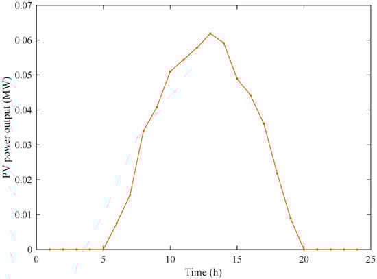
Figure 1.
Baseline data of PV power output.
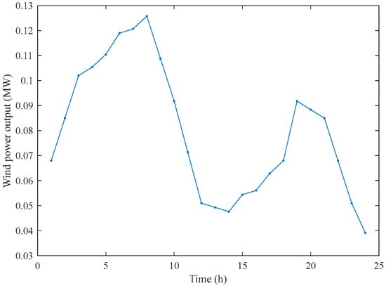
Figure 2.
Baseline data of wind power output.
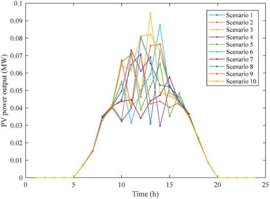
Figure 3.
Typical scenario of PV power output.
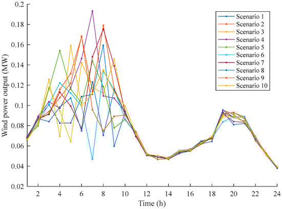
Figure 4.
Typical scenario of wind power output.
3. Optimal Allocation Model for DG
The allocation model of DG can be divided into a two-layer model including the investment level and the operation level. This study integrates the correlation modeling of the investment level and the operation level. Meanwhile, the uncertainty of wind and solar power outputs and DR is considered. The structure of the allocation problem is shown in Figure 5.
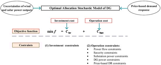
Figure 5.
The structure of DG allocation problem.
3.1. Objective Function
The objective function includes the investment cost (CInv) and the operation cost (COper). The overall objective function is as follows.
where f is the total cost.
In this paper, DG includes wind-turbine generation (WTG), photovoltaic generation and micro-turbine generation (MTG). The total investment cost of the three DGs is considered, represented as follows,
where CWTG, CPV and CMTG represent the investment cost of WTG, PV and MTG, respectively.
The investment cost of WTG is shown below.
The investment cost of PV is shown below.
The investment cost of MTG is shown below.
The operation costs include the cost of purchasing electricity from the main grid (CP), network loss cost (Closs), penalty costs of wind power (CWTG,cur) and solar power curtailed (CPV,cur), cost of energy not supplied (CENS), MTG generation cost (CMTG,Ope) and DR cost (CDR). Details of the operation costs above are described as follows.
3.2. Constraints
3.2.1. Investment Constraints
The DG installation is restricted by the maximum installation limitation at each DG candidate bus as follows.
3.2.2. Operation Constraints
- (a)
- Power flow constraints.
- (b)
- Security constraints.
- (c)
- Substation power constraints.
- (d)
- DG power constraints.
- (e)
- Price-based DR constraints.
DR can promote the allocation of DG by peak shaving and valley filling of loads and improving the renewable energy accommodation. Specifically, the price-based DR shows a very flexible incentive function for loads based on the electricity price. Therefore, the price-based DR based on elasticity is used in this paper, shown below.
4. Problem Reformulation
As can be seen, DR cost involves non-linear terms. Meanwhile, the constraints (15)–(17) are all non-linear terms, which are difficult to solve. Therefore, the non-linear term should be transformed.
4.1. Reformulation of the Net Annual Profit
The net annual profit is bilinear. The electricity price and load will vary around the initial price and load. So, the Taylor series expansion method is used to address the bilinear term. A tractable form is reformulated around as follows.
The corresponding DR cost is shown below.
4.2. Reformulation of the Power Flow Model
For the non-linear term in the power flow model, the auxiliary variable is introduced. Then, the power flow model can be shown below.
The security constraint is shown below,
where , , , are all auxiliary variables shown below.
After the above settlement, it is still difficult to solve the allocation model. This is because Equation (28) is non-convex. The second-order conic relaxation method is used to reformulate it. The reformulation model is shown below.
5. Case Studies
A modified IEEE 33-bus system including residential, commercial and industrial consumers is used to validate the proposed model (see Figure 6). The simulations are implemented by CPLEX 12.6.0 using MATLAB R2016b on a personal computer with an Intel Core (i7, 1.80 GHz) and 16 GB memory. The price of power purchasing from a main grid, i.e., the transmission price, is 78 USD/MWh. The capital costs of WTG, PV and MTG are 85,000 USD/unit, 65,000 USD/unit and 95,000 USD/unit, respectively, and their capacities are 0.2 (WTG), 0.1 (PV) and 0.3 (MTG) MW. The initial preference prices of residential, commercial and industrial consumers are 86.67 USD/MWh, 91.23 USD/MWh and 79.33 USD/MWh, respectively. The elastic coefficients are shown in Table 1. The other parameters used in this paper are listed in Table 2.
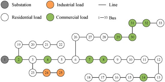
Figure 6.
The 33-bus test system.

Table 1.
Elastic coefficients.
Table 2.
Parameters involved in solving the model.
5.1. Impact of DR on Planning Results
Two cases are carried out to analyze the impact of demand response on the planning results of DG. Case 1 is carried out without DR, while Case 2 involves DR. The DR capacity is set to 15% of load. The corresponding planning results are shown in Table 3.
Table 3.
Comparison of different planning schemes in different Cases.
As can be seen from Table 3, the invested numbers of PV are 17 and 20 in Cases 1 and 2, respectively. The penetration capacities of PV are 1.7 MW and 2 MW, respectively. For WTG, the invested numbers are 14 and 17 in Cases 1 and 2, respectively, while its penetration capacities are 2.8 MW and 3.4 MW, respectively. So, DR can increase both the invested number and penetration capacity of PV and WTG. However, the curtailed costs of wind power and PV power are USD 0.2742 × 10⁶ and USD 0.1089 × 10⁶, respectively, in Case 2, higher than those in Case 1 (USD 0.2642 × 10⁶ and USD 0.0991 × 10⁶). This is because the invested numbers of both PV and WTG in Case 2 are larger than those in Case 1.
To fully investigate the impact of DR on the accommodation of renewable energy, the curtailed costs of wind power and PV power per unit (106 USD/unit) are introduced. The curtailed cost of wind power (PV power) per unit is defined as the ratio of the curtailed cost of wind power (PV power) to the invested numbers of WTG and PV. In this way, the curtailed cost of wind power (PV power) per unit in Cases 1 and 2 are 0.0189 × 10⁶ USD/unit (0.0058 × 10⁶ USD/unit) and 0.0161 × 10⁶ USD/unit (0.0054 × 10⁶ USD/unit), respectively. So, the accommodation of renewable energy can be improved by DR.
In addition, as shown in Table 3, the DR cost in Case 2 is negative, which indicates that the power company has gained benefits after implementing DR. Meanwhile, it can also be seen that the network loss cost in Case 2 is USD 0.5088 × 10⁶, which is smaller than that in Case 1 (USD 0.5865 × 10⁶). This means that implementing the DR project can improve network flow and reduce system network loss. However, Case 2 results in a certain degree of loss of load. This is because users reduce the use of certain types of energy-generating equipment on the same day under certain extreme conditions such as high electricity prices.
In addition, it can be seen that the annual comprehensive cost of Case 2 is USD 5.4946 × 10⁶, which is less than that of Case 1 (USD 6.6600 × 10⁶). This indicates that the annual investment and operating costs of the power company can be greatly saved after implementing DR. This is because the invested amount of DG in Case 2 is higher than that in Case 1, which increases the annual investment cost of DG. Meanwhile, the curtailed costs of wind and solar power also increase. There is a certain degree of loss of load in Case 2, which the power company bears. However, the benefits obtained by implementing DR can completely offset or even exceed the costs paid, while the corresponding compensation can be obtained. Therefore, the total cost of Case 2 is smaller than that of Case 1.
5.2. Impact of DR on Load Curves
To further analyze the load curve after taking into account demand response, several load curves for different types of loads in the same scenario are given. Specifically, the total load curve is given in Figure 7. The load curves of residential load in node 3, commercial load in node 4 and industrial load in node 24 are given in Figure 7, Figure 8, Figure 9 and Figure 10, respectively.
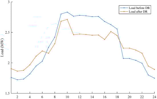
Figure 7.
Total load curve.
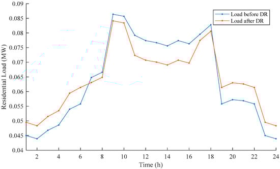
Figure 8.
Residential load curve.
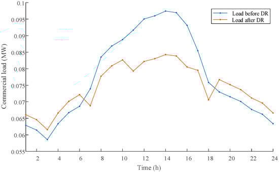
Figure 9.
Commercial load curve.
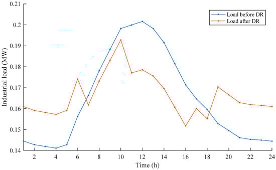
Figure 10.
Industrial load curve.
From Figure 7, Figure 8, Figure 9 and Figure 10, it can be seen that after implementing DR, the peak load of the system decreases. Meanwhile, the load from 7:00 to 18:00 is smaller than that before implementing DR. The system load during the period from 19:00 to 7:00 significantly increases. Due to the decrease in peak load, the probability of security threats faced by the system decreases, which improves the system security. This is because after implementing DR, in order to reduce the network loss cost of the system and the security threats faced by the system, the power company sets the electricity price higher during the 7:00–18:00 period to reduce user electricity consumption. During the 19:00–7:00 period, the power company sets the electricity price lower to stimulate users to increase their electricity consumption. In this way, the reduced electricity consumption of the power company during the 7:00–18:00 period can be compensated, which reduces the power company’s losses.
After the comparison of different user load curves, it can be seen that after the implementation of the DR project, the daily electricity consumption curves of the three types of users have all shown a phenomenon of peak load reduction and valley load increase, known as the “peak shaving and valley filling” phenomenon. This fully indicates that electricity prices have a certain attraction to all three types of users and all three types of users have participated in demand response. However, it is not difficult to see that the degree of change in the load curves of the three types of users is different. Specifically, industrial users change the most while the degree of change for residential users is the smallest. This is because the elasticity of different users is different. As shown in Table 2, industrial users have the highest elasticity coefficient, while residential users have the smallest elasticity coefficient. Therefore, among the three types of users, industrial users have the highest participation in demand response, while residential users have the lowest participation in demand response.
5.3. Impact of DR Capacity Limit on Planning Results
The upper limit of DR capacity was set for each user to 5%, 15% or 25% of the predicted load for comparative analysis. The planning results are shown in Table 4.
Table 4.
Comparison of different planning schemes in different DR capacity limit.
From Table 4, it can be seen that as the upper limit of DR response capacity increases, the more negative the DR cost is; that is, the more benefits the power company can gain from implementing DR. And the annual total cost gradually decreases. At the same time, the installation number and penetration capacity of PV increase while the total power curtailed cost decreases. These changes indicate that the larger the upper limit of DR response capacity is, the stronger the system’s accommodation capacity of photovoltaics can be made via the implementation of DR. On the other hand, the installation quantity and penetration capacity of WTGs decrease with an increase in the upper limit of DR response capacity. The cost of wind curtailment also decreases. However, the unit cost of wind curtailment is USD 0.0174 × 10⁶, USD 0.0161 × 10⁶ and USD 0.0150 × 10⁶, respectively. It can be seen that the system’s accommodation ability for wind power also increases. This is mainly because an increase in the upper limit of DR response capacity characterizes the enhanced ability of users to participate in demand response. As the DR response capacity limit increases, the load that users can transfer to the night also increases. In this situation, the ability to absorb wind power can also be improved.
In addition, it can be seen that as the DR capacity limit increases, the system’s network loss cost continues to decrease while the cost of loss of load continues to increase. This indicates that increasing the DR capacity limit can better improve the system’s operation and reduce network loss. But at the same time, the situation of loss of load will also become more severe. So, it is necessary to allocate DR capacity reasonably to balance the loss of load and the consumption of clean energy.
6. Conclusions
This paper considers the impact of demand response based on real-time electricity prices on the allocation scheme of distributed generations in the distribution network. The demand response cost is introduced as one of the optimization objectives. The allocation model of DG is solved after linearizing the non-linear terms in the model. The conclusions are shown below.
- (1)
- DR can improve the allocation of DG by improving the renewable energy accommodation ability of a distribution network. Meanwhile, DR can also increase the profits of the power company and significantly reduce the annual total cost of the power company when planning distributed generations in the distribution network. The network flow of the system can be improved and network losses reduced. However, the system may experience a loss of load as a result.
- (2)
- DR shows a significant effect on peak shaving and valley filling. Compared with the planning results without DR, DR can significantly adjust the system load curve and user electricity consumption habits. Different types of users have different sensitivities to electricity prices, resulting in varying degrees of participation in demand response. Residential users have the smallest sensitivity to electricity prices while industrial users are the most sensitive to electricity prices.
- (3)
- The DR response capacity limit has a significant impact on optimization results. The larger the upper limit of DR response capacity is, the higher the system’s accommodation of renewable energy is. However, an increase in the upper limit of the DR response capacity may cause more severe system load loss and even generate new peak loads. The probability of encountering security threats in the system may increase, which affects the safe and stable operation of the system. Therefore, it is necessary to reasonably consider DR response capacity.
The assumed empirical distribution of wind power and PV power is uncertain. So, the allocation method considering the probability distribution of wind power and PV power will be further studied in the future. In addition, the impact of the flexibility of renewable energy on the allocation of DG will be further studied in the future.
Author Contributions
Conceptualization, S.H.; Methodology, S.H.; Writing—original draft, S.H.; Supervision, J.L. All authors have read and agreed to the published version of the manuscript.
Funding
This work was supported by the Key Laboratory of Modern Power System Simulation and Control & Renewable Energy Technology (Northeast Electric Power University) Open Fund under Grant MPSS2023-09.
Data Availability Statement
Data are contained within the article.
Conflicts of Interest
The authors declare no conflict of interest.
Nomenclature
| Abbreviations | |
| DG | Distributed generation. |
| DR | Demand response. |
| MTG | Micro-turbine generation. |
| PV | Photovoltaic generation. |
| RO | Robust optimization. |
| SO | Stochastic optimization. |
| WTG | Wind-turbine generation. |
| Indices | |
| i, j, k | Index of buses. |
| ij, ki | Index of lines. |
| s | Index of scenarios. |
| t, t′ | Index of time slots. |
| Sets | |
| // //// | Bus set of WTG/PV/MTG/system node/load/substation/lines. |
| Parameters | |
| Own elasticity or cross elasticity. | |
| Price before demand response. | |
| / | The upper/lower limits of price. |
| / | Price to transmission/power losses. |
| / | Price to load loss/MTG generation power. |
| // | Capital cost of WTG/PV/MTG. |
| / | Price of WTG power curtailment/PV power curtailment. |
| The upper limit of current. | |
| lki/lij | Length of line ki/ij. |
| Number of total scenarios. | |
| // | The maximal installation number of WTG/PV/MTG. |
| Probability value of each scenario. | |
| Active load before demand response. | |
| / | The upper limits of active/reactive power injected by the substation. |
| / | The upper/lower limits of active load after demand response. |
| / | The upper/lower limits of active power of MTG. |
| / | Forecast power of WTG/PV in typical scenarios. |
| r | Discount rate |
| Rij, Rki/Xij, Xki | Resistance/reactance of line ij/ki. |
| / | The upper/lower limits of voltage. |
| The lifespan of DG. | |
| Variables | |
| Price after demand response. | |
| / | Current of line ki/ij. |
| / | Active/reactive load after demand response. |
| Power losses through line ij. | |
| / | Active/reactive power of PV. |
| / | Active/reactive power of MTG. |
| , /, | Active/reactive power of line ij/ki. |
| / | Active/reactive power injected by the substation. |
| / | Active/reactive power of WTG. |
| Integer variables; numbers of some elements (WTG, PV and MTG) | |
| / | Voltage at node i/j. |
| , /, | Auxiliary variables; square of branch current branch and bus voltage. |
References
- Salama, H.S.; Magdy, G.; Bakeer, A.; Vokony, I. Adaptive coordination control strategy of renewable energy sources, hydrogen production unit, and fuel cell for frequency regulation of a hybrid distributed power system. Prot. Control Mod. Power Syst. 2022, 7, 34. [Google Scholar] [CrossRef]
- Uma, U.U.; Nmadu, D.; Ugwuanyi, N.; Ogah, O.E.; Eli-Chukwu, N.; Eheduru, M.; Ekwue, A. Adaptive overcurrent protection scheme coordination in presence of distributed generation using radial basis neural network. Prot. Control Mod. Power Syst. 2023, 8, 1–19. [Google Scholar] [CrossRef]
- Shu, H.; Li, W.; Wang, G.; Han, Y.; Li, J.; Tang, Y. Online Collaborative Estimation Technology for SOC and SOH of Frequency Regulation of a Lead-Carbon Battery in a Power System with a High Proportion of Renewable Energy. Prot. Control Mod. Power Syst. 2024, 9, 52–64. [Google Scholar] [CrossRef]
- Zhang, D.; Shafiullah, G.M.; Das, C.K.; Wong, K.W. A systematic review of optimal planning and deployment of distributed generation and energy storage systems in power networks. J. Energy Storage 2022, 56, 105937. [Google Scholar] [CrossRef]
- Xu, B.; Zhang, G.; Li, K.; Li, B.; Chi, H.; Yao, Y.; Fan, Z. Reactive power optimization of a distribution network with high-penetration of wind and solar renewable energy and electric vehicles. Prot. Control Mod. Power Syst. 2022, 7, 51. [Google Scholar] [CrossRef]
- He, Q.; Lin, Z.; Chen, H.; Dai, X.; Li, Y.; Zeng, X. Bi-level optimization based two-stage market clearing model considering guaranteed accommodation of renewable energy generation. Prot. Control Mod. Power Syst. 2022, 7, 30. [Google Scholar] [CrossRef]
- Fathabad, A.M.; Cheng, J.; Pan, K.; Qiu, F. Data-driven planning for renewable distributed generation integration. IEEE Trans. Power Syst. 2020, 35, 4357–4368. [Google Scholar] [CrossRef]
- Kumar, S.; Manjrekar, V.; Singh, V.; Lad, B.K. Integrated yet distributed operations planning approach: A next generation manufacturing planning system. J. Manuf. Syst. 2020, 54, 103–122. [Google Scholar] [CrossRef]
- Ali, Z.M.; Diaaeldin, I.M.; El-Rafei, A.; Hasanien, H.M.; Aleem, S.H.A.; Abdelaziz, A.Y. A novel distributed generation planning algorithm via graphically-based network reconfiguration and soft open points placement using Archimedes optimization algorithm. Ain Shams Eng. J. 2021, 12, 1923–1941. [Google Scholar] [CrossRef]
- Rigo-Mariani, R.; Vai, V. An iterative linear distflow for dynamic optimization in distributed generation planning studies. Int. J. Electr. Power Energy Syst. 2022, 138, 107936. [Google Scholar] [CrossRef]
- Bai, W.; Zhang, W.; Allmendinger, R.; Enyekwe, I.; Lee, K.Y. A Comparative Study of Optimal PV Allocation in a Distribution Network Using Evolutionary Algorithms. Energies 2024, 17, 511. [Google Scholar] [CrossRef]
- Prakash, R. Optimal Distributed Generation Planning Considering Economic and Operational Aspects. Electr. Power Compon. Syst. 2023, 1–16. [Google Scholar] [CrossRef]
- Ding, X.; Xu, J.; Sun, Y.; Liao, S.; Zheng, J. A demand side controller of electrolytic aluminum industrial microgrids considering wind power fluctuations. Prot. Control Mod. Power Syst. 2022, 7, 49. [Google Scholar] [CrossRef]
- Fan, D.; Zhang, S.; Huang, H.; Zhou, L.; Wang, Y.; Xiao, X. Three-stage day-ahead scheduling strategy for regional thermostatically controlled load aggregators. Prot. Control Mod. Power Syst. 2023, 8, 19. [Google Scholar] [CrossRef]
- Gao, H.; Wang, R.; He, S.; Wang, Z.; Liu, J. Bi-level Stackelberg game-based distribution system expansion planning model considering long-term renewable energy contracts. Prot. Control Mod. Power Syst. 2023, 8, 62. [Google Scholar] [CrossRef]
- Koutsoukis, N.C.; Georgilakis, P.S. A multistage distribution network planning method considering distributed generation active management and demand response. IET Renew. Power Gener. 2022, 16, 65–76. [Google Scholar] [CrossRef]
- Dang, C.; Wang, X.; Shao, C.; Wang, X. Distributed generation planning for diversified participants in demand response to promote renewable energy integration. J. Mod. Power Syst. Clean Energy 2019, 7, 1559–1572. [Google Scholar] [CrossRef]
- Melgar-Dominguez, O.D.; Pourakbari-Kasmaei, M.; Lehtonen, M.; Mantovani, J.R.S. An economic-environmental asset planning in electric distribution networks considering carbon emission trading and demand response. Electr. Power Syst. Res. 2020, 181, 106202. [Google Scholar] [CrossRef]
- Xu, W.; Zhou, D.; Huang, X.; Lou, B.; Liu, D. Optimal allocation of power supply systems in industrial parks considering multi-energy complementarity and demand response. Appl. Energy 2020, 275, 115407. [Google Scholar] [CrossRef]
- He, S.; Gao, H.; Tian, H.; Wang, L.; Liu, Y.; Liu, J. A two-stage robust optimal allocation model of distributed generation considering capacity curve and real-time price based demand response. J. Mod. Power Syst. Clean Energy 2020, 9, 114–127. [Google Scholar] [CrossRef]
- Fu, X. Statistical machine learning model for capacitor planning considering uncertainties in photovoltaic power. Prot. Control Mod. Power Syst. 2022, 7, 5. [Google Scholar] [CrossRef]
- Fu, X.; Wu, X.; Zhang, C.; Fan, S.; Liu, N. Planning of distributed renewable energy systems under uncertainty based on statistical machine learning. Prot. Control Mod. Power Syst. 2022, 7, 41. [Google Scholar] [CrossRef]
- Xiao, D.; Chen, H.; Cai, W.; Wei, C.; Zhao, Z. Integrated risk measurement and control for stochastic energy trading of a wind storage system in electricity markets. Prot. Control Mod. Power Syst. 2023, 8, 1–11. [Google Scholar] [CrossRef]
- Wang, J.; Xie, N.; Huang, C.; Wang, Y. Two-stage stochastic-robust model for the self-scheduling problem of an aggregator participating in energy and reserve markets. Prot. Control Mod. Power Syst. 2023, 8, 1–20. [Google Scholar] [CrossRef]
- Roy, T.K.; Ghosh, S.K.; Saha, S. Robust backstepping global integral terminal sliding mode controller to enhance dynamic stability of hybrid AC/DC microgrids. Prot. Control Mod. Power Syst. 2023, 8, 8. [Google Scholar] [CrossRef]
- Yin, M.; Li, K.; Yu, J. A data-driven approach for microgrid distributed generation planning under uncertainties. Appl. Energy 2022, 309, 118429. [Google Scholar] [CrossRef]
- Jin, W.; Zhang, S.; Li, J. Robust planning of distributed generators in active distribution network considering network reconfiguration. Appl. Sci. 2023, 13, 7747. [Google Scholar] [CrossRef]
- Bazrafshan, M.; Yalamanchili, L.; Gatsis, N.; Gomez, J. Stochastic planning of distributed PV generation. Energies 2019, 12, 459. [Google Scholar] [CrossRef]
- Ehsan, A.; Yang, Q. Coordinated investment planning of distributed multi-type stochastic generation and battery storage in active distribution networks. IEEE Trans. Sustain. Energy 2018, 10, 1813–1822. [Google Scholar] [CrossRef]
- Sunderland, K.; Woolmington, T.; Blackledge, J.; Conlon, M. Small wind turbines in turbulent (urban) environments: A consideration of normal and Weibull distributions for power prediction. J. Wind Eng. Ind. Aerodyn. 2013, 121, 70–81. [Google Scholar] [CrossRef]
- Lei, K.; Chang, J.; Wang, X.; Guo, A.; Wang, Y.; Ren, C. Peak shaving and short-term economic operation of hydro-wind-PV hybrid system considering the uncertainty of wind and PV power. Renew. Energy 2023, 215, 118903. [Google Scholar] [CrossRef]
Disclaimer/Publisher’s Note: The statements, opinions and data contained in all publications are solely those of the individual author(s) and contributor(s) and not of MDPI and/or the editor(s). MDPI and/or the editor(s) disclaim responsibility for any injury to people or property resulting from any ideas, methods, instructions or products referred to in the content. |
© 2024 by the authors. Licensee MDPI, Basel, Switzerland. This article is an open access article distributed under the terms and conditions of the Creative Commons Attribution (CC BY) license (https://creativecommons.org/licenses/by/4.0/).