

Evaluation of FACTS Contributions Using Branch Flow Model and Newton–Raphson Algorithm


Abstract
1. Introduction
2. NR and OPF with FACTS Devices
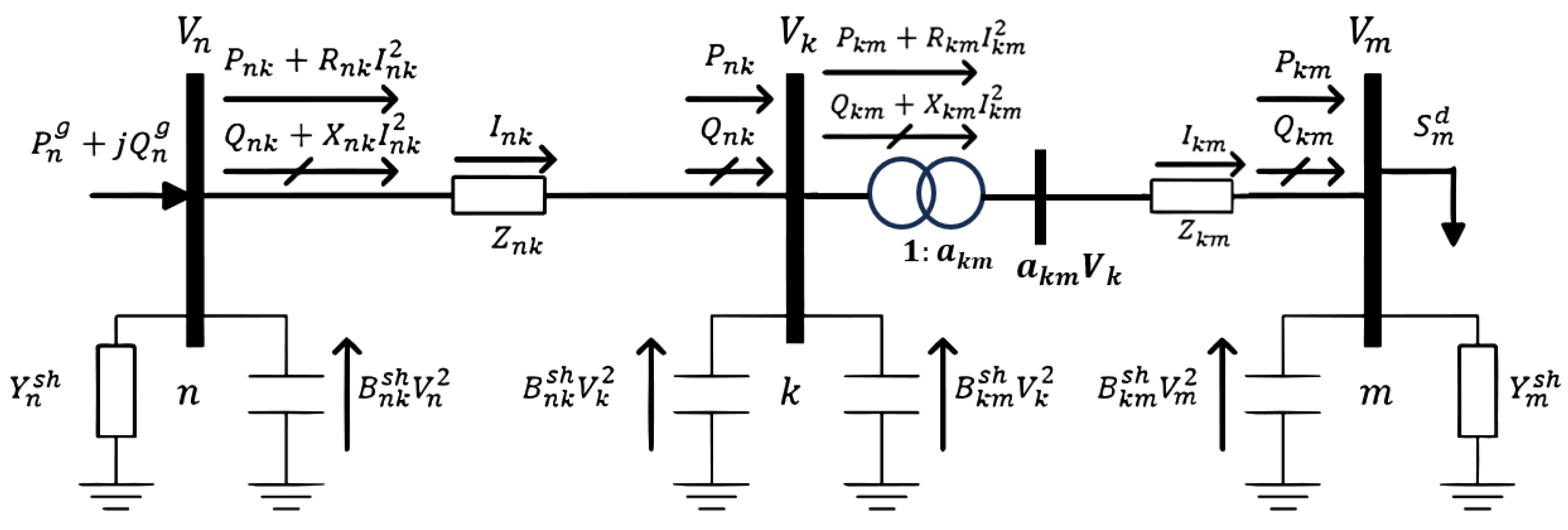
2.1. AC Power Flow Model
- The negative term represents the active power drained as losses from the shunt element.
- The sum of the terms represents the power flows, including losses, going out of bus k to the neighboring bus m connected through branch km.
- 3.
- The term represents the reactive power of the uncontrolled shunt element.
- 4.
- must be positive when injecting power in capacitive behavior, and must be negative when absorbing power in inductive behavior.
- 5.
- The sum of terms denotes the power flows reaching bus from its neighboring bus connected through branch , including half of the power input represented at the arriving end due to the capacitive effect of the transmission line.
- 6.
- The sum of the terms represents the power flows leaving bus towards the neighboring bus connected by branch , which includes half of the power input represented at the output end due to the capacitive effect of the transmission line plus the losses from this.
2.2. SVC—Firing Angle Model
2.2.1. Newton–Raphson Algorithm with SVC
2.2.2. OPF with SVC
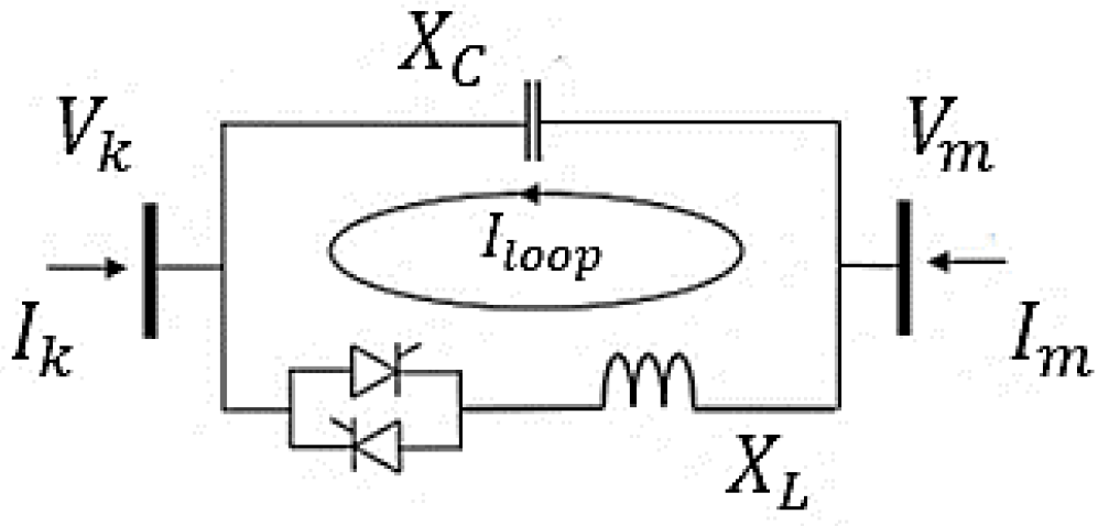
2.3. TCSC—Firing Angle Model
2.3.1. Newton–Raphson Algorithm with TCSC
2.3.2. OPF with TCSC
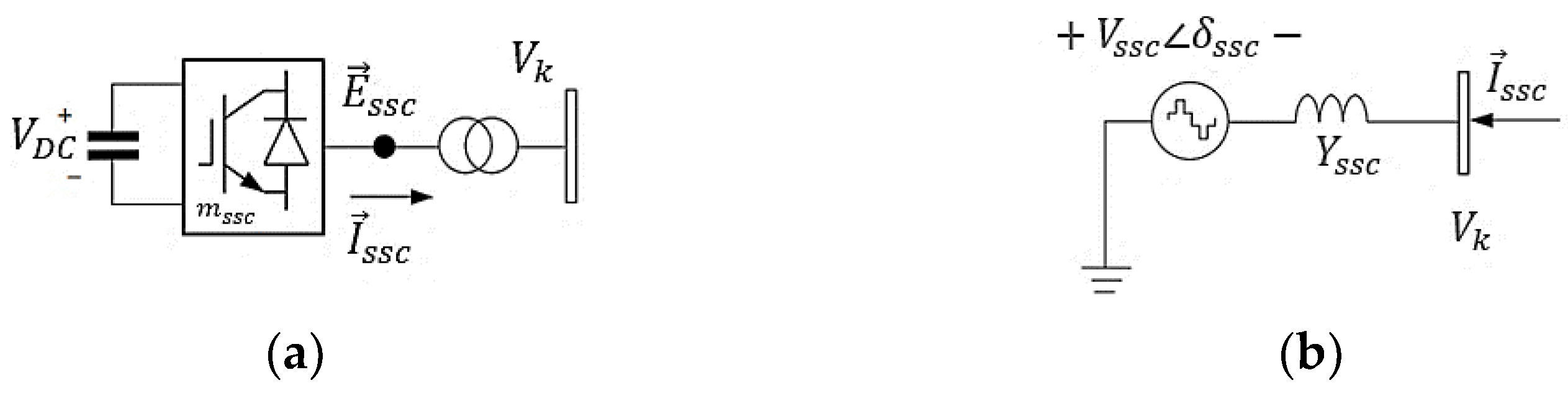
2.4. STATCOM
2.4.1. Newton–Raphson Algorithm with STATCOM
2.4.2. OPF with STATCOM
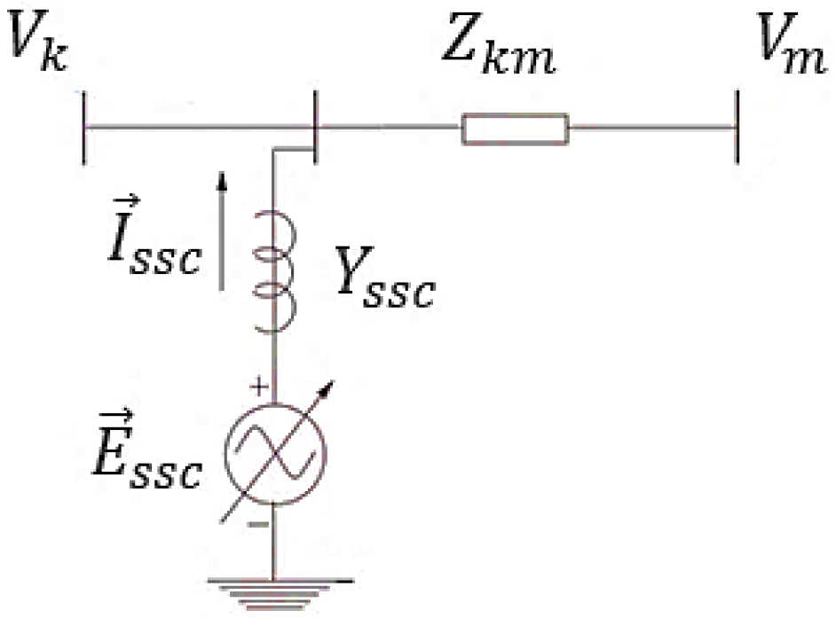
2.5. SSSC
OPF with SSSC
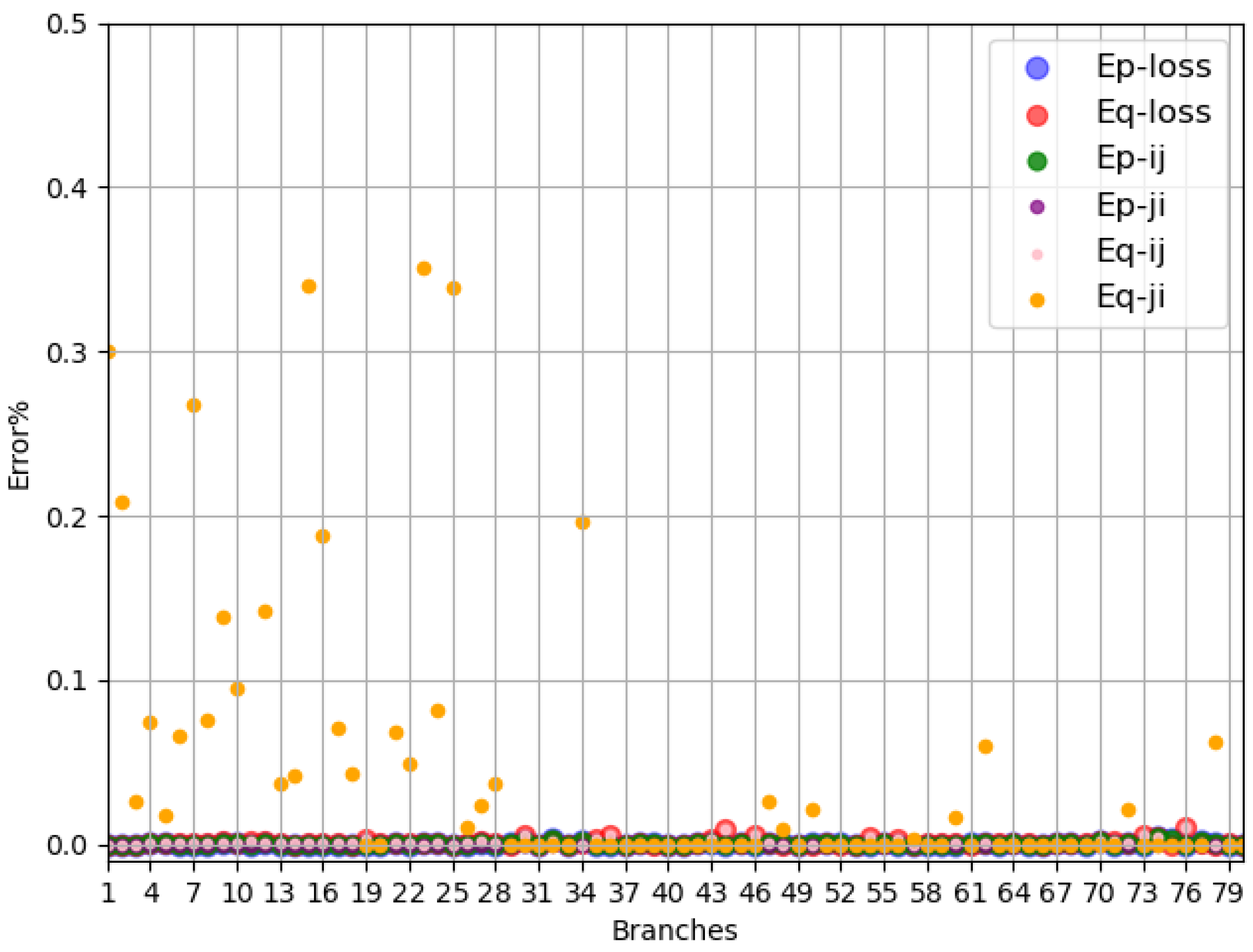
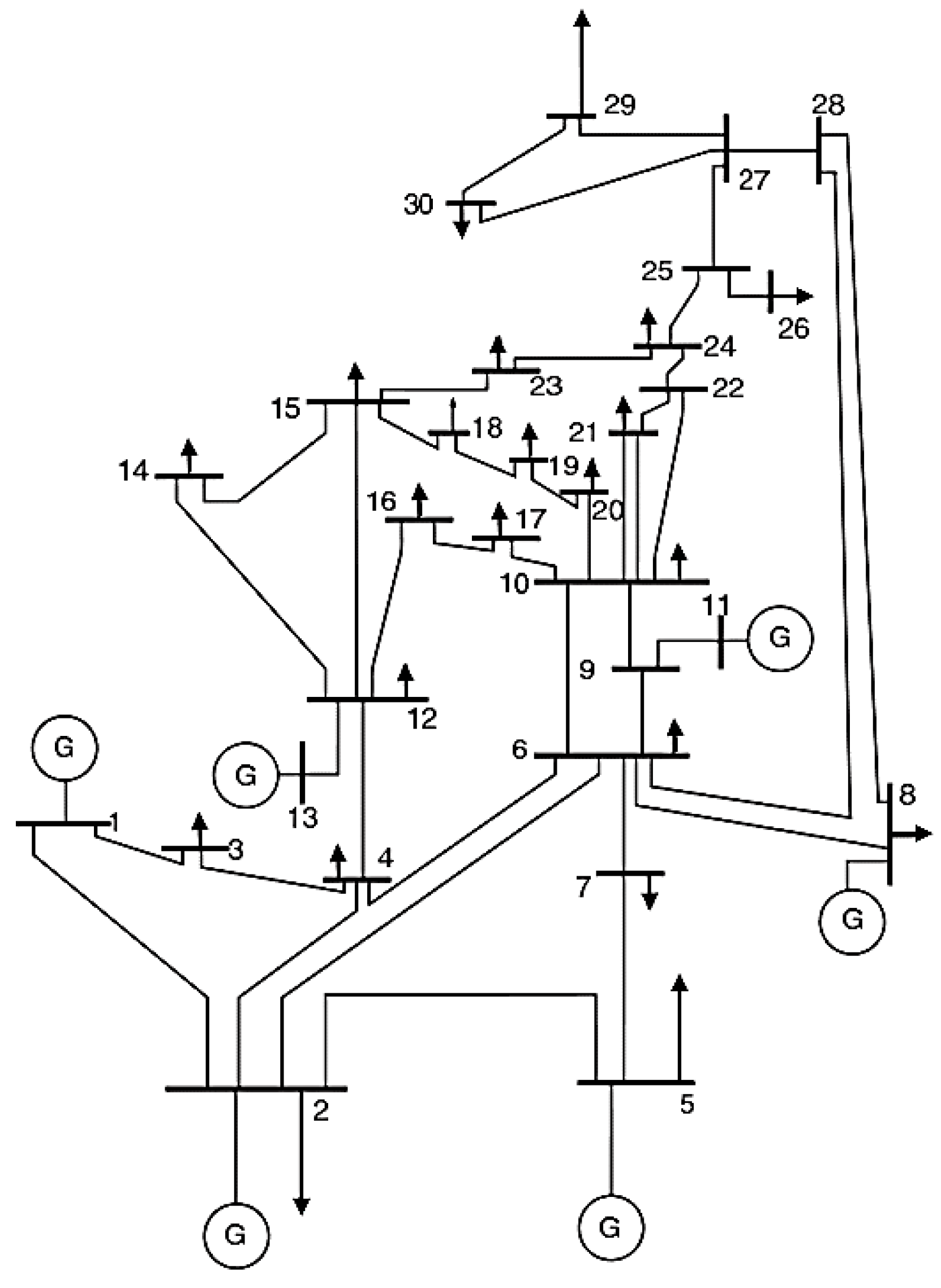
3. Numerical Results
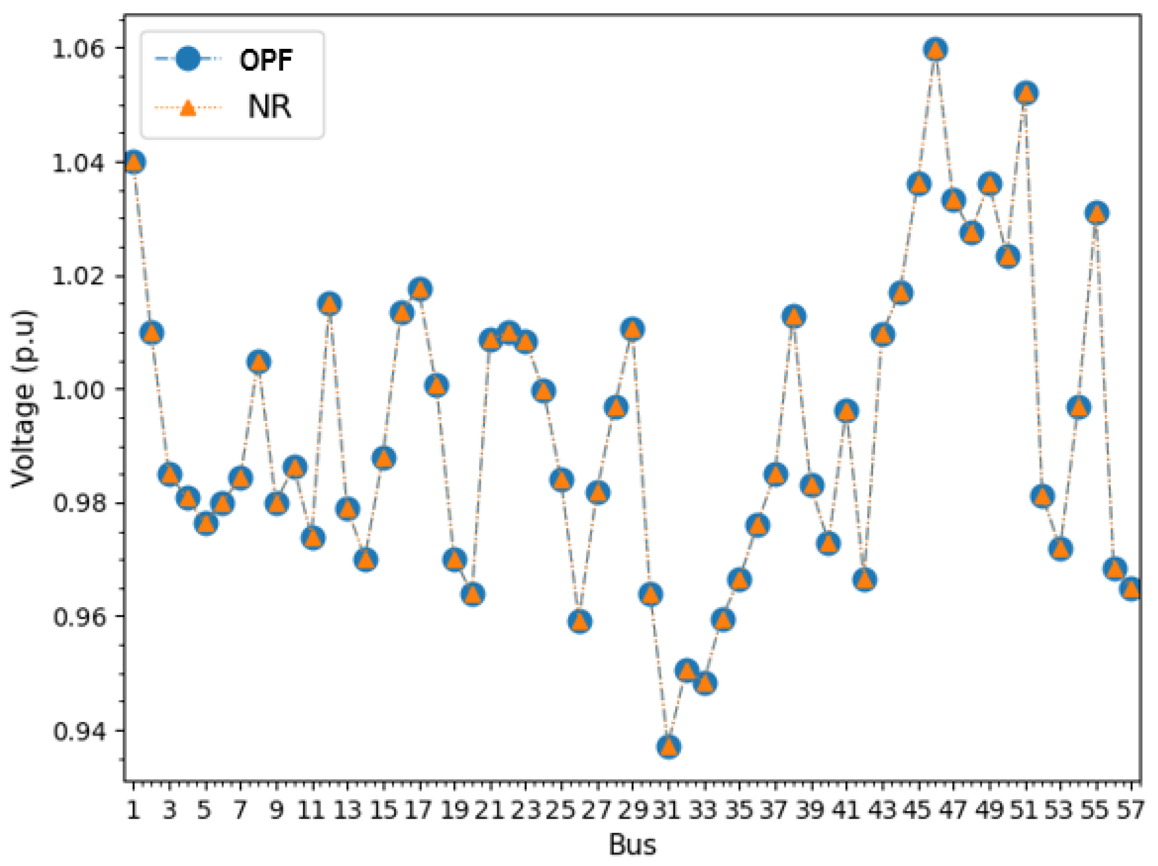
3.1. Base Case
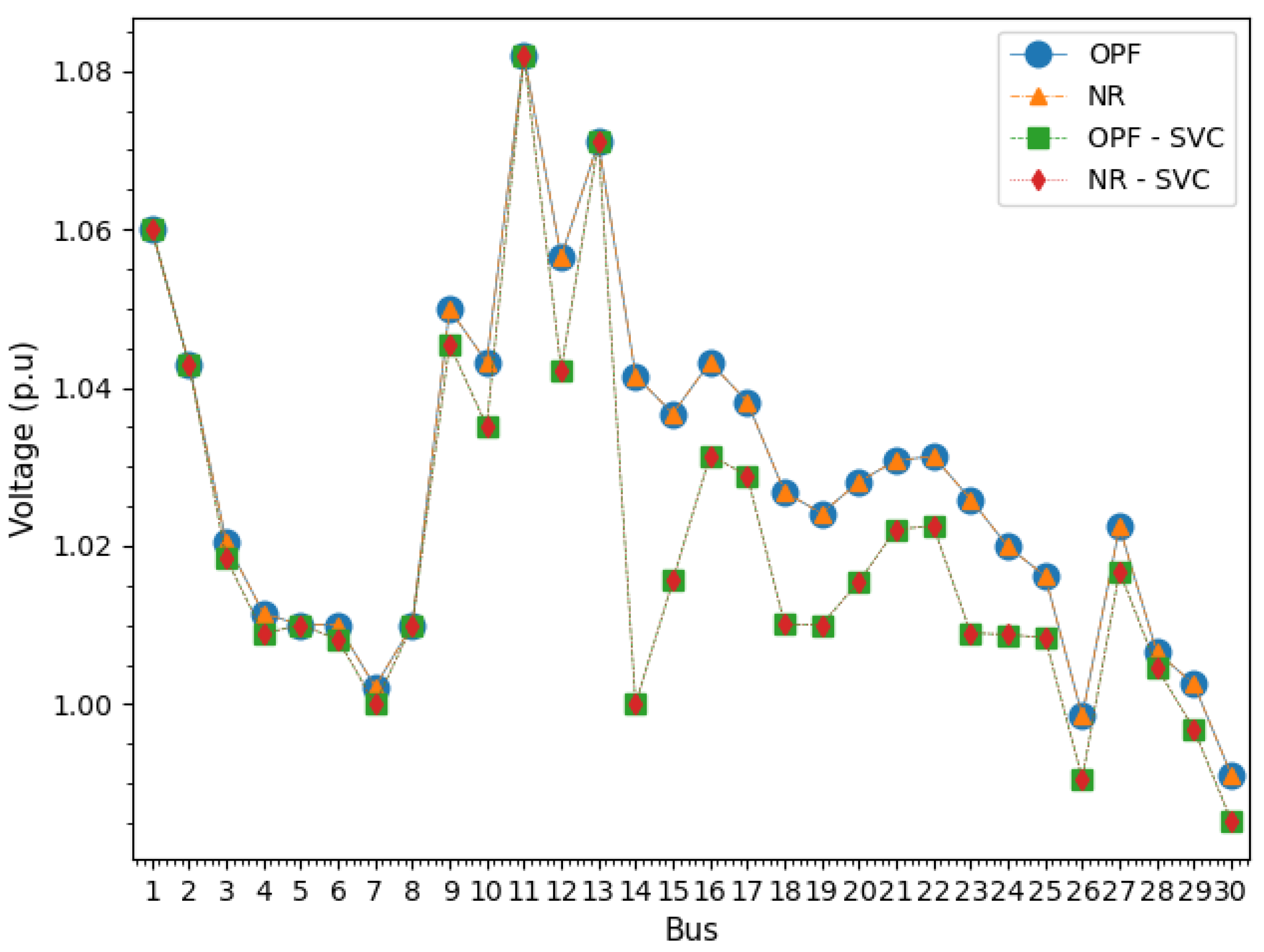
3.2. Case with SVC
3.3. Case with STATCOM
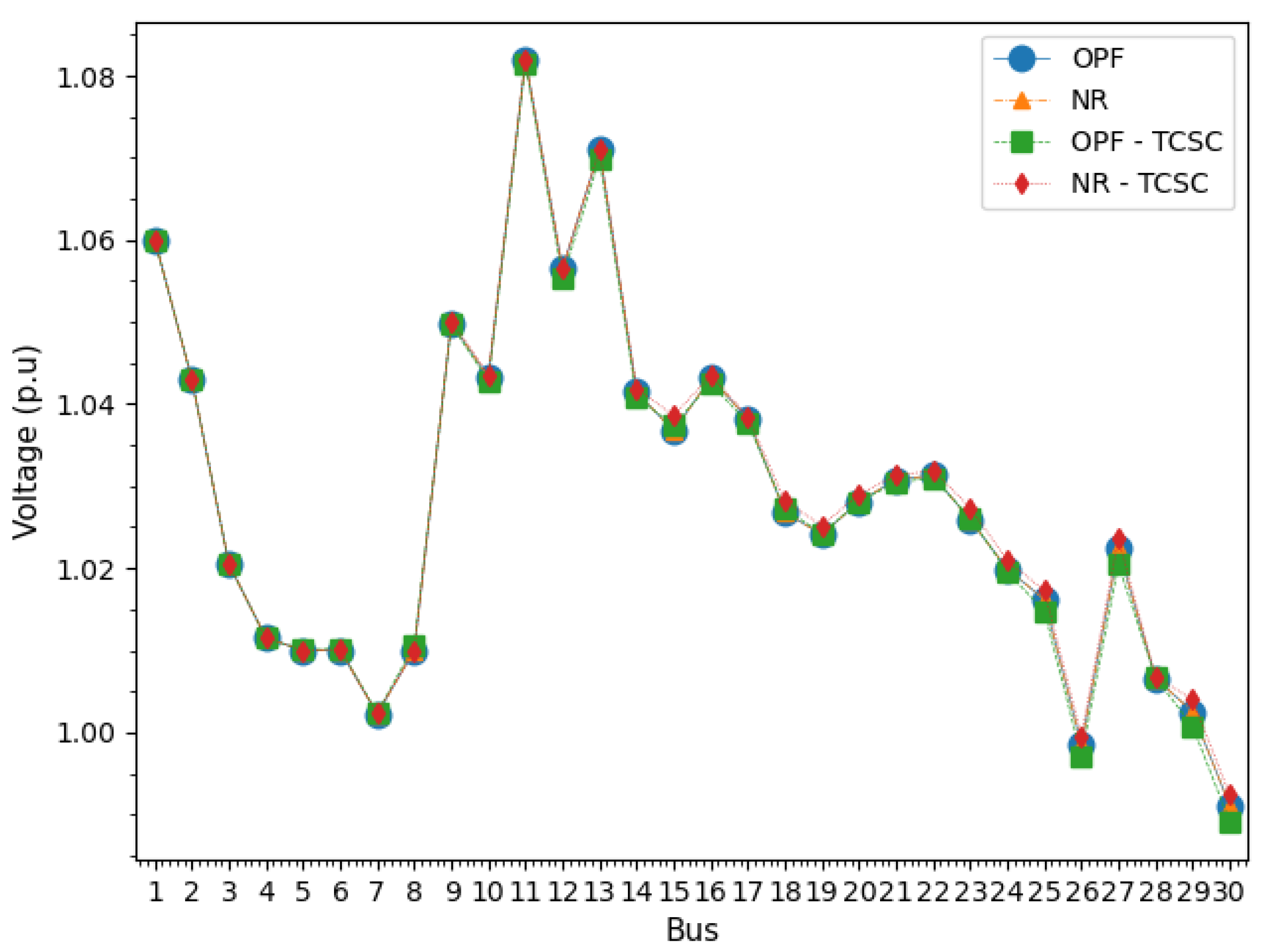
3.4. Case with TCSC
3.5. Case with SSSC
4. Discussion
5. Conclusions
Author Contributions
Funding
Data Availability Statement
Conflicts of Interest
References
- Watnabe, E.H.; Barbosa, P.G.; Almeida, K.C.; Taranto, G.N. TECNOLOGIA FACTS–TUTORIAL. SBA Controle Autom. 1998, 9, 39–55. [Google Scholar]
- Hingorani, N.G.; Gyugyi, L. Understanding FACTS: Concepts and Technology of Flexible AC Transmission Systems; IEEE: New York, NY, USA, 1999. [Google Scholar]
- Hingorani, N.G. High Power Electronics and flexible AC Transmission System. IEEE Power Eng. Rev. 1988, 8, 3–4. [Google Scholar] [CrossRef]
- Hingorani, N.G. Power electronics in electric utilities: Role of power electronics in future power systems. Proc. IEEE 1988, 76, 481–482. [Google Scholar] [CrossRef]
- Larson, E.; Weaver, T. FACTS Overview; IEEE/CIGRE; Springer: Berlin/Heidelberg, Germany, 1995. [Google Scholar]
- Pérez, H.A. Flexible AC Transmission Systems Modelling in Optimal Power Flows Using Newton’s Method; Department of Electronics and Electrical Engineering, University of Glasgow: Glasgow, UK, 1997. [Google Scholar]
- Luburić, Z.; Pandžić, H. FACTS Devices and Energy Storage in Unit Commitment. Int. J. Electr. Power Energy Syst. 2019, 104, 311–325. [Google Scholar] [CrossRef]
- Ghiasi, M. Technical and economic evaluation of power quality performance using FACTS devices considering renewable generations. Renew. Energy Focus 2019, 29, 49–62. [Google Scholar] [CrossRef]
- Chawda, G.S.; Shaik, A.G.; Mahela, O.P.; Padmanaban, S.; Holm-Nielse, J.B. Comprehensive review of distributed FACTS control algorithms for power quality enhancement in utility grid with renewable energy penetration. IEEE Access 2020, 8, 107614–107634. [Google Scholar] [CrossRef]
- Nadeem, M.; Imran, K.; Khattak, A.; Ulasyar, A.; Pal, A.; Zeb, M.Z.; Khan, A.N.; Padhee, M. Optimal Placement, Sizing and Coordination of FACTS Devices in Transmission Network Using Whale Optimization Algorithm. Energies 2020, 13, 753. [Google Scholar] [CrossRef]
- Valle, D.B.; Araujo, P.B. The influence of GUPFC FACTS device on small signal stability of the electrical power systems. Int. J. Electr. Power Energy Syst. 2015, 65, 299–306. [Google Scholar] [CrossRef]
- Pomilio, J.A.; Paredes, H.K.; Deckmann, S.M. Eletrônica de Potência no Sistema de Transmissão: Dispositivos FACTS; UNICAMP: Campinas, Brazil, 2013. [Google Scholar]
- Andersen, B.R.; Nilsson, S.L. Flexible AC Transmission Systems. In CIGRE Green Books; Springer: Berlin/Heidelberg, Germany, 2020. [Google Scholar]
- Gyugyi, L. Power electronics in electric utilities: Static VAR compensators. Proc. IEEE 1988, 76, 483–494. [Google Scholar] [CrossRef]
- Fuerte-Esquivel, C.R.; Acha, E.; Ambriz-Perez, H. A thyristor-controlled series compensator model for the power flow solution of practical power networks. IEEE Trans. Power Syst. 2000, 15, 58–64. [Google Scholar] [CrossRef]
- Singh, B.; Al-Haddad, K.; Saha, R.; Chanda, A. Static synchronous compensators (STATCOM): A review. IET Power Electron. 2009, 2, 297–324. [Google Scholar] [CrossRef]
- Sen, K.K. SSSC-static synchronous series compensator: Theory, modeling, and application. IEEE Trans. Power Deliv. 1998, 13, 241–246. [Google Scholar] [CrossRef]
- Gyugyi, L. Unified power-flow control concept for flexible AC transmission systems. Proc. Inst. Electr. Eng. Part C Gener. Transmiss. Distrib. 1992, 139, 323–331. [Google Scholar] [CrossRef]
- Gyugyi, L.; Sen, K.; Schauderr, C.D. The interline power flow controller concept: A new approach to power flow management in transmission systems. IEEE Trans. Power Deliv. 1999, 14, 1115–1123. [Google Scholar] [CrossRef]
- Zhang, X.P.; Handschin, E.; Yao, M. Modeling of the generalized unified power flow controller (GUPFC) in a nonlinear interior point OPF. Power Syst. IEEE Trans. 2001, 16, 367–373. [Google Scholar] [CrossRef]
- Monticelli, A.J. Fluxo de Carga Em Redes de Energia Eletrica; Edgar Bucher: São Paulo, Brazil, 1983. [Google Scholar]
- Naderi, E.; Pourakbari-Kasmaei, M.; Abdi, H. An efficient particle swarm optimization algorithm to solve optimal power flow problem integrated with FACTS devices. Appl. Soft Comput. 2019, 80, 243–262. [Google Scholar] [CrossRef]
- Ahmad, A.A.; Sirjani, R. Optimal placement and sizing of multi-type FACTS devices in power systems using metaheuristic optimisation techniques: An updated review. Ain Shams Eng. J. 2019, 11, 611–628. [Google Scholar] [CrossRef]
- LakshmiPriya, J.; Jaya Christa, S.T. An effective hybridized GWOBSA for resolving optimal power flow problem with the inclusion of unified power flow controller. IETE J. Res. 2021, 69, 1–13. [Google Scholar]
- Muhammad, Y.; Khan, R.; Raja, M.A.Z.; Ullah, F.; Chaudhary, N.I.; He, Y. Solution of optimal reactive power dispatch with FACTS devices: A survey. Energy Rep. 2020, 6, 2211–2229. [Google Scholar] [CrossRef]
- Carpentier, J. Optimal power flows. Int. J. Electr. Power Energy Syst. 1979, 1, 3–15. [Google Scholar] [CrossRef]
- Cain, M.B.; O’Neill, R.P.; Castillo, A. History of optimal power flow and formulations (OPF Paper 1). Fed. Energy Regul. Comm. 2012, 1, 1–36. [Google Scholar]
- Ribeiro, P.M. Remuneração Dos Serviços Ancilares de Reserva de Potência E Suporte de Potência Reativa Quando Providos Por Geradores. Master’s Thesis, Pontifícia Universidade Católica do Rio de Janeiro, Rio de Janeiro, Brazil, 2004. [Google Scholar]
- Stevenson, J.W.; Grainger, J. Power System Analysis; McGraw-Hill: New York, NY, USA, 1994. [Google Scholar]
- Farivar, M.; Low, S.H. Branch flow model: Relaxations and convexification—Part I. IEEE Trans. Power Syst. 2013, 28, 2554–2564. [Google Scholar] [CrossRef]
- Macedo, L.H.; Montes, C.V.; Franco, J.F.; Rider, M.J.; Romero, R. MILP branch flow model for concurrent ac multistage transmission expansion and reactive power planning with security constraints. IET Gener. Transmiss. Distrib. 2016, 10, 3023–3032. [Google Scholar] [CrossRef]
- Baran, M.E.; Wu, F.F. Optimal capacitor placement on radial distribution systems. IEEE Trans. Power Del. 1989, 4, 725–734. [Google Scholar] [CrossRef]
- Fuerte Esquivel, C.R. Steady State Modelling and Analysis of Flexible AC Transmission Systems; Department of Electronics and Electrical Engineering, University of Glasgow: Glasgow, UK, 1997. [Google Scholar]
- Acha, E.; Fuerte-Esquiel, C.R.; Ambriz-Perez, H. Advanced SVC model for Newton-Raphson load flow and Newton optimal power flow studies. IEEE Trans. Power Syst. 2000, 15, 129–136. [Google Scholar]
- Acha, E.; Fuerte-Esquivel, C.R.; Ambriz-Perez, H.; Angeles-Camacho, C. FACTS: Modelling and Simulation in Power Networks; Wiley: Hoboken, NJ, USA, 2004. [Google Scholar]
- Menniti, D.; Burgio, A.; Pinnarelli, A.; Scordino, N.; Sorrentino, N. Steady state security analysis in presence of UPFC Corrective actions. In Proceedings of the 2002 of Power Systems Computation Conference, Sevilla, Spain, 24–28 June 2002. Session 17, paper 5. [Google Scholar]
- Noroozian, M.; Angquist, L.; Ghandhari, M.; Andersson, G. Use of UPFC for optimal power flow control. IEEE Trans Power Del. 1997, 12, 1629–1634. [Google Scholar] [CrossRef]
- Voraphonpiput, N.; Bunyagu, T. Power Flow Control with Static Synchronous Series Compensator (SSSC). Int. Energy J. 2008, 9, 117–127. [Google Scholar]
- Zhang, X.P. Advanced modeling of the multicontrol functional static synchronous series compensator (SSSC) in Newton power flow. IEEE Trans. Power Syst. 2003, 18, 1410–1416. [Google Scholar] [CrossRef]
- Peyghami, S.; Davari, P.; Fotuhi-Firuzabad, M.; Blaabjerg, F. Standard test systems for modern power system analysis: An overview. IEEE Ind. Electron. Mag. 2019, 13, 86–105. [Google Scholar] [CrossRef]


| 5 Bus System | IEEE 14-Bus System | IEEE 30-Bus System | IEEE 57-Bus System | |
|---|---|---|---|---|
| Nodes | 5 | 14 | 30 | 57 |
| Transmission lines | 7 | 15 | 34 | 63 |
| Transformers | 0 | 5 | 7 | 17 |
| Generators | 1 | 4 | 5 | 6 |
| Loads | 4 | 11 | 21 | 42 |
| Shunt compensator | 0 | 1 | 2 | 3 |
| Slack node | 1 | 1 | 1 | 1 |
| Minimum voltage | 0.9 | 0.9 | 0.9 | 0.9 |
| Maximum voltage | 1.1 | 1.1 | 1.1 | 1.1 |
| Test System | Bus | NR | Branch Flow Model | Error | ||||||||
|---|---|---|---|---|---|---|---|---|---|---|---|---|
| Magnitude (p.u) | Angle (°) | Losses (MW) | MPT (Seg) | Magnitude (p.u) | Angle (°) | Losses (MW) | MPT (Seg) | Magnitude (%) | Losses (%) | MPT (%) | ||
| 5 buses | 1 | 1.060 | 0.000 | 6.122 | 0.139 | 1.060 | 0.000 | 6.122 | 0.091 | 0.000 | 0.000 | 34.517 |
| 2 | 1.000 | −2.061 | 1.000 | −2.061 | 0.000 | |||||||
| 3 | 0.987 | −4.636 | 0.987 | −4.636 | 0.000 | |||||||
| 4 | 0.984 | −4.957 | 0.984 | −4.957 | 0.000 | |||||||
| 5 | 0.971 | −5.764 | 0.971 | −5.764 | 0.000 | |||||||
| IEEE 14 buses | 1 | 1.060 | 0.000 | 13.401 | 0.148 | 1.060 | 0.000 | 13.408 | 0.114 | 0.000 | 0.049 | 22.871 |
| 2 | 1.045 | −4.982 | 1.045 | −4.983 | 0.000 | |||||||
| 3 | 1.010 | −12.726 | 1.010 | −12.726 | 0.000 | |||||||
| 6 | 1.070 | −14.240 | 1.071 | −14.245 | 0.093 | |||||||
| 8 | 1.090 | −13.348 | 1.088 | −13.435 | 0.100 | |||||||
| IEEE 30 buses | 1 | 1.060 | 0.000 | 17.562 | 0.150 | 1.060 | 0.000 | 17.562 | 0.119 | 0.000 | 0.000 | 26.671 |
| 2 | 1.043 | −5.350 | 1.043 | −5.353 | 0.000 | |||||||
| 5 | 1.010 | −14.168 | 1.010 | −14.182 | 0.000 | |||||||
| 8 | 1.010 | −11.815 | 1.010 | −11.838 | 0.000 | |||||||
| 11 | 1.082 | −14.103 | 1.082 | −14.422 | 0.000 | |||||||
| 13 | 1.071 | −14.957 | 1.071 | −15.551 | 0.000 | |||||||
| IEEE 57 buses | 1 | 1.040 | 0.000 | 27.845 | 0.191 | 1.040 | 0.000 | 27.845 | 0.149 | 0.000 | 0.001 | 21.998 |
| 2 | 1.010 | −1.188 | 1.010 | −1.188 | 0.000 | |||||||
| 3 | 0.985 | −5.987 | 0.985 | −5.987 | 0.010 | |||||||
| 6 | 0.980 | −8.674 | 0.980 | −8.674 | 0.020 | |||||||
| 8 | 1.005 | −4.477 | 1.005 | −4.477 | 0.009 | |||||||
| 9 | 0.980 | −9.584 | 0.980 | −9.584 | 0.010 | |||||||
| 12 | 1.015 | −10.470 | 1.015 | −10.470 | 0.029 | |||||||
| System | NR | Branch Flow Model | Error (%) | |||
|---|---|---|---|---|---|---|
| Losses (MW) | MPT (s) | Losses (MW) | MPT (s) | Losses | MPT | |
| 5 buses | 6.056 | 0.275 | 6.055 | 0.144 | 0.000 | 47.645 |
| 14 buses | 13.919 | 0.272 | 13.934 | 0.189 | 0.110 | 30.518 |
| 30 buses | 18.152 | 0.286 | 18.152 | 0.185 | 0.000 | 35.313 |
| 57 buses | 27.846 | 0.302 | 27.846 | 0.219 | 0.000 | 27.487 |
| System | NR | Branch Flow Model | Error (%) | |||
|---|---|---|---|---|---|---|
| Losses (MW) | MPT (s) | Losses (MW) | MPT (s) | Losses | MPT | |
| 5 buses | 6.056 | 0.282 | 6.055 | 0.166 | 0.000 | 41.131 |
| 14 buses | 13.919 | 0.288 | 13.934 | 0.184 | 0.110 | 36.117 |
| 30 buses | 18.152 | 0.279 | 18.152 | 0.217 | 0.000 | 22.223 |
| 57 buses | 27.846 | 0.294 | 27.846 | 0.223 | 0.000 | 24.157 |
| System | NR | Branch Flow Model | Error (%) | |||
|---|---|---|---|---|---|---|
| Losses (MW) | MPT (s) | Losses (MW) | MPT (s) | Losses | MPT | |
| 5 buses | 6.127 | 0.195 | 6.127 | 0.154 | 0.000 | 13.85 |
| 14 buses | 13.481 | 0.200 | 13.475 | 0.1 | 0.041 | 14.504 |
| 30 buses | 17.653 | 0.215 | 17.661 | 0.183 | 0.053 | 14.883 |
| 57 buses | 27.901 | 0.235 | 27.879 | 0.201 | 0.080 | 14.475 |
| System | NR | Branch Flow Model | Error (%) | |||
|---|---|---|---|---|---|---|
| Losses (MW) | MPT (s) | Losses (MW) | MPT (s) | Losses | MPT | |
| 5 buses | 6.127 | 0.195 | 6.127 | 0.154 | 0.000 | 21.031 |
| 14 buses | 13.481 | 0.200 | 13.475 | 0.169 | 0.041 | 15.506 |
| 30 buses | 17.653 | 0.215 | 17.661 | 0.193 | 0.053 | 10.237 |
| 57 buses | 27.901 | 0.235 | 27.879 | 0.215 | 0.080 | 8.511 |
Disclaimer/Publisher’s Note: The statements, opinions and data contained in all publications are solely those of the individual author(s) and contributor(s) and not of MDPI and/or the editor(s). MDPI and/or the editor(s) disclaim responsibility for any injury to people or property resulting from any ideas, methods, instructions or products referred to in the content. |
© 2024 by the authors. Licensee MDPI, Basel, Switzerland. This article is an open access article distributed under the terms and conditions of the Creative Commons Attribution (CC BY) license (https://creativecommons.org/licenses/by/4.0/).
Share and Cite
Corpus, M.J.T.; Leite, J.B. Evaluation of FACTS Contributions Using Branch Flow Model and Newton–Raphson Algorithm. Energies 2024, 17, 918. https://doi.org/10.3390/en17040918
Corpus MJT, Leite JB. Evaluation of FACTS Contributions Using Branch Flow Model and Newton–Raphson Algorithm. Energies. 2024; 17(4):918. https://doi.org/10.3390/en17040918
Chicago/Turabian StyleCorpus, Marco Junior Ticllacuri, and Jonatas B. Leite. 2024. "Evaluation of FACTS Contributions Using Branch Flow Model and Newton–Raphson Algorithm" Energies 17, no. 4: 918. https://doi.org/10.3390/en17040918
APA StyleCorpus, M. J. T., & Leite, J. B. (2024). Evaluation of FACTS Contributions Using Branch Flow Model and Newton–Raphson Algorithm. Energies, 17(4), 918. https://doi.org/10.3390/en17040918