Abstract
The intermittent and volatile nature of wind power generation necessitates thermal power units to provide deep-peak shaving and fast frequency regulation services within the same grid. However, the current proportional integral differential (PID) control performance in the process control foundation of thermal power units falls short of meeting these requirements. Despite the lack of comprehensive research on engineering fastest control (EFC), this article aims to address this gap by studying and analyzing the mechanism and physical defects of the fast tracking filter (FTF), the output tracking input characteristics of EFTF reconstructed by FTF engineering, and the control performance of the constructed EFC. Through mathematical calculation analysis, simulation experiments, and real-world engineering practice, it is concluded that EFC surpasses the limitations of PID control performance and effectively enhances feedback control performance. As a result, it is deemed suitable for process control in thermal power units.
1. Introduction
The electric power industry plays a vital role in providing the energy needed for various industries. It serves as a foundational industry that is closely tied to the national economy, people’s livelihoods, and national strategies. The power system itself is a vast network consisting of three main components: power generation, power transmission and distribution through the power grid, and power consumption by end-users. The power generation side encompasses a diverse range of technologies, including coal-fired thermal power generation [1], gas power generation [2], hydropower generation [3], nuclear power generation [4], wind power generation [5], and photovoltaic power generation [6], among others. These different power generation systems coexist, forming a complex network to meet the energy demands of society. Hydropower, wind power, photovoltaic power generation, and so on are renewable resources, which also include biomass power generation [7], tidal power generation [8], and so on.
The production process of thermal power generation is a typical industry process. The typical process involves the following steps: Water, coal, and air enter the boiler, where they undergo combustion to generate high-pressure steam. This steam then drives a turbine, which in turn powers a generator to produce electricity. With the increasing concern about energy conservation and environmental protection, thermal power units have undergone significant advancements in terms of efficiency, capacity, and operating parameters. A large-scale thermal power unit involves various control aspects, including machine–boiler coordination control, water supply control, combustion control, wind pressure and temperature control, steam temperature control, and environmental protection control. The number of control loops is around 100 to 120 due to the inherent complexity of thermal power generation.
Over recent years, the automatic control of thermal power units has made remarkable progress, reaching a high level of sophistication and effectiveness. This progress has been driven by the continuous development and refinement of control systems and technologies, enabling more efficient and reliable operation of thermal power units.
Industrial control technology, including the control technology for thermal power units, is intricately linked to the advancement of control science. The increasing demands of industrial control drive the progress and development of control science, while the evolution of control science presents a multitude of options for selecting and implementing industrial control technologies. Regrettably, it is noteworthy that traditional proportional–integral–derivative (PID) control [9,10,11,12], including proportional–integral (PI) control, continues to dominate the field of thermal power unit control. Despite the potential for further advancements, the prevalent use of PID control in this context suggests that alternative control methods have yet to gain widespread adoption. Reference [13] points out that “PID based feedback control remains a preferred basic control technology in the field of industrial process control, including thermal power unit process control”. Indeed, despite the advancements in control theory research, the position of PID control as a preferred basic control technology in the field of industrial control remains steadfast. This observation highlights a discernible gap between control theory research and its practical application in control engineering.
With the proposal of carbon peaking and carbon neutrality goals, new energy represented by wind power and photovoltaic solar power is rapidly developing in China. The peak in carbon emissions refers to the highest value of carbon emissions. With the continued development of new energy, carbon emissions begin to decrease after reaching the peak. One of the main drawbacks of renewable energy sources is their intermittent and unstable nature. The integration of new energy into the power grid poses security challenges that cannot be ignored. In order to address this issue, the power grid needs to rapidly enhance its capabilities for peak load adjustment and frequency regulation. Thermal power units serve as the fundamental components of the power generation side in global power systems.
The existing literature [13] highlights the significant improvement in deep-peak adjustment and rapid frequency regulation performance, achieved by optimizing the control systems of current thermal power units. Improving the peak adjustment and frequency regulation capabilities represents the primary task at this stage. The realization of deep-peak adjustment and rapid frequency regulation performance in existing thermal power units involves measures such as reducing the response time when changing the magnitude of boiler wind, coal, and water, or raising the unit load rate.
However, these rapid changes in wind, coal, water, and unit load rates inevitably result in significant fluctuations in important process parameters of thermal power units, such as the main steam pressure, main steam temperature, and heating steam temperature. From the perspective of these notable fluctuations in vital process parameters, it is evident that the current PID control foundation in thermal power units is insufficient to meet these control requirements. Consequently, in practical applications, it is necessary to replace the existing PID control with more advanced alternatives.
In 2018, researchers made a significant breakthrough in engineering practice by introducing the engineering fastest tracking filter (EFTF) as a potential replacement for PID control [13]. This innovation laid the foundation for the development of the engineering fastest control (EFC) [13], which represents a novel industrial process control technology that greatly enhances feedback control performance. By 2023, EFC had successfully replaced PID control on a large scale in a commercial renovation project involving the auxiliary frequency modulation of thermal power units in Guangdong province [13,14] in China.
Auxiliary frequency modulation [13,14] is an auxiliary control strategy proposed to facilitate the integration of renewable energy sources into the power grid, aligning with China’s goals of the carbon peak and carbon neutrality. Under the auxiliary frequency modulation mode, the load command of thermal power units is subjected to increased randomness. With the output of renewable energy sources, the thermal power units are controlled to ramp up their output rapidly and randomly, and vice versa. This approach ensures that the power grid frequency remains within the designated range. Auxiliary frequency modulation plays a vital and irreplaceable role in facilitating the widespread utilization of renewable energy within the power grid and ensuring its safe and stable operation during the transition.
The existing literature indeed lacks comprehensive research and analysis on engineering fastest control (EFC). The main contribution of this study is to unveil the theoretical foundation that EFC can significantly enhance feedback control performance. Additionally, this study provides a mathematical optimization method for determining PID and EFC parameters with robust performance. Furthermore, it presents a relatively complete engineering tuning method for EFC parameters.
The expressions used for functions, parameters, and variables in this study are unique and can be cross-referenced. To maintain conciseness, unless otherwise stated, the following units are used: time in seconds (s), the time constant in seconds (s), acceleration in meters per square second (m/s2), frequency in radians per second (rad/s), the phase stability margin in degrees (°), proportional gain in dimensionless units, order in dimensionless units, and logarithmic gain in decibels (dB).
2. The Deficiencies of PID Control and the Essential Problems Revealed in Engineering Practice
PID control has been widely employed in various industrial process control applications, including thermal power unit control. However, it is evident that PID control has certain limitations, particularly in terms of dynamic control accuracy. Over time, researchers have continuously explored different avenues to improve PID control. Some notable advancements include optimal PID control [9], PID control based on output compensation [10], auto-PID control [11], and fractional-order PID control [12].
According to reference [15], a significant flaw in PID control has been uncovered, specifically regarding the inefficiency of conventional integral control when tracking constant perturbations. This inefficiency stems from the nature of conventional integrals. In PID control, the integrator represents a conventional integrator (CI).
The research highlights the importance of low-pass filters (LPFs) in constructing controllers, with the PID structure being based on a first-order inertial filter (FOIF) [15]. The FOIF structure relies on an exponential tracking filtering mechanism, where the output tracks the input at an exponential rate. This exponential control mechanism is a fundamental characteristic of PID control. The underlying issue of low efficiency in conventional integration is determined by the FOIF filtering mechanism, which is integral to the construction of PID control. The intuitive performance of the FOIF mechanism reveals a low efficiency in tracking the input with the output.
Prior to the development of engineering fastest control (EFC), researchers in the field of engineering recognized the fundamental issue of the inefficiency of conventional integration. As a result, they proposed the concept of a fastest tracking filter (FTF) [13]. Building upon this, a novel feedback controller (NFC) [15] was devised to implement a maximum control mechanism. However, in practical engineering applications, it was discovered that the performance of the NFC was not able to match that of PID control, suggesting the existence of other essential problems within NFC.
During the engineering practice of the NFC, researchers identified the physical limitations of the fastest tracking filter (FTF). In controller design, the advanced observer [13] serves as a fundamental component, and it is common in practice to construct a high-performance advanced observer through inverse transformations. For instance, the proportional–integral (PI) controller is obtained by inversely transforming the FOIF proportional–derivative (PD) controller. Additionally, the application of PD control in the structure of the PID controller can significantly enhance the overall performance of PID control. However, the inverse FTF transformation contains pure hysteresis, and the advanced observation of pure hysteresis is physically unrealizable, which causes the physical defects of FTF. However, without the addition of high-performance advanced observers, the NFC control performance is not enough to compete with PID control.
In engineering practice, researchers proposed an inertial combined filter (ICF) [13] in order to overcome the physical defects of FTF. The principle of the FTF engineering reconstruction method is to use the characteristics of the ICF to approximate the FTF, and the ICF engineering reconstruction results of the FTF are obtained from the EFTF.
The FOIF, FTF and EFTF [13] are
where and are, respectively, the transfer functions and time constants of the FOIF. and are, respectively, the transfer functions and window time constants of the FTF. , and are, respectively, the transfer functions, time constants, and engineering reconstruction orders of the EFTF.
In engineering, cannot be infinite, and the default in this study is .
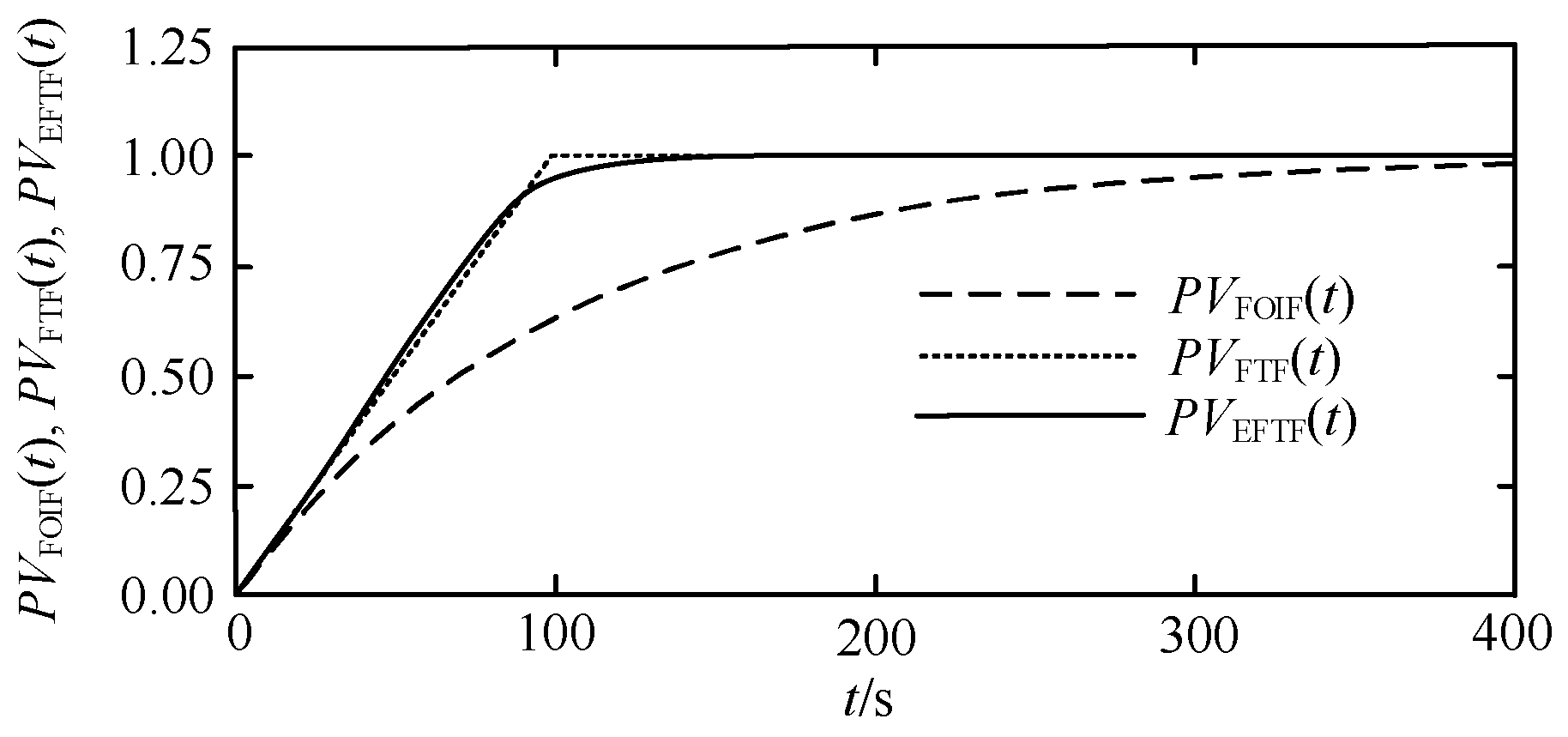
The FOIF, FTF, and EFTF are kinds of low-pass filter. In , there is an intuitive understanding of the characteristics of the FOIF, FTF, and EFTF and the input unit step to obtain the FOIF, FTF, and EFTF process output, , , and , as shown in Figure 1 [13].

Figure 1.
A diagram of low-pass filter process output.
As illustrated in Figure 1, the engineering fastest tracking filter (EFTF) exhibits notable improvements in output tracking compared to the FOIF. It not only inherits the favorable characteristics of the FTF but also addresses the physical limitations of the FTF. This makes it a suitable tool for constructing advanced observers with high performance.
It is important to note that the inefficiency of conventional integral control in tracking constant perturbations, the physical limitations of the FTF, and the engineering enhancements made to the FTF are the essential problems that engineering researchers have uncovered in their practical work. However, it is crucial to acknowledge that these issues do not encompass all the essential problems encountered in the field of control engineering.
3. Engineering Fastest Control
EFC involves the engineering fastest proportion–integral (EFPI) [13] controller and the engineering fastest leading observer (EFLO) [13]. The EFPI and EFLO are based on the EFTF.
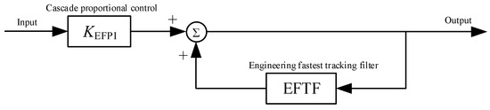
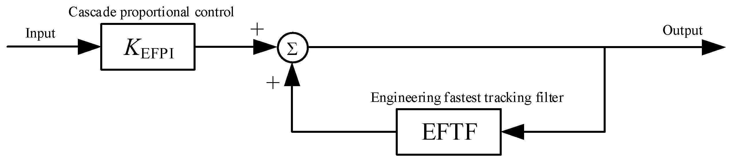
Figure 2.
The diagram of EFPI.
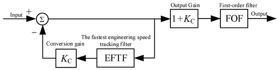
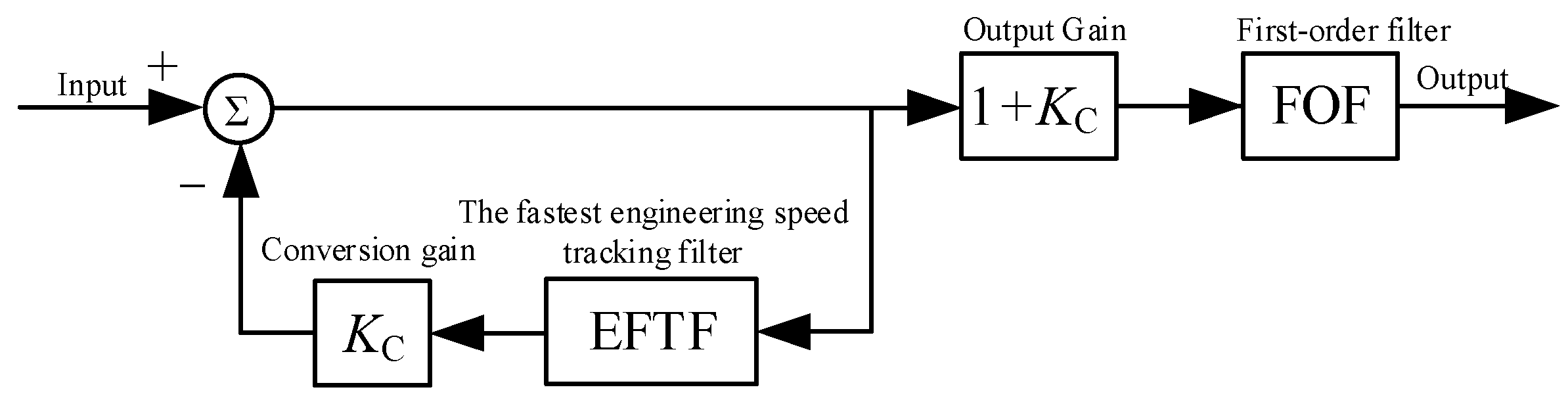
Figure 3.
The diagram of EFLO.
The EFPI and EFLO [13] are
where and are, respectively, the transfer functions and cascade proportional gains of the EFPI. and are, respectively, the engineering fastest integrator (EFI) transfer function and integration time constant. Numerically, , , , and are, respectively, the transfer functions, transform gains, and time constants of the EFLO. TFOF is the time constant of the first-order filter (FOF) and the quantity of .
The EFI is a generalized integrator [16] which uses the relative zero frequency gain (RZFG) of the EFI and CI to measure the integration efficiency of the EFI.
The RZFG [13] is expressed as
where and are the frequency domain functions of the EFI and CI. When and tends to 0, the RZFG of the EFI is 1.882 times higher than that of the CI.
Equation (3) shows that the EFI significantly improves the efficiency of integration compared with the CI.
For the sake of comparison, the PID adopts the cascade structure of PI and PD, and the PID is
where , , and are, respectively, the transfer functions of PID, PI, and PD. and are, respectively, the proportional gain and integration time constants of PI. and are, respectively, the differential time constants of PD and the time constants of the second-order filter (SOF).
The EFLO and PD mainly have the problem of noise interference amplification. The problem of noise interference amplification is important, but there is no standard for how to measure the noise interference amplification characteristics. The noise power gain (NPG) of the advanced observer is proposed in Ref. [13]. Qualitatively speaking, an NPG of 10 or below is a low noise interference level. In the EFLO and PD, the basic reason for setting and is to ensure that the NPG of the EFLO and PD is equal to or below 10. When the NPG = 10, the peak phase of the EFLO is 82.7° and the gain is 17.9 dB. The peak phase of PD is 54.4° and the gain is 19.9 dB. The comparison results of EFC and PID in this study are obtained under the condition of NPG = 10.
NPG is expressed as
Among them, is the noise interference output, is the noise interference input, and is the time length of the calculation of the NPG. The default is in this text.
In terms of EFC parameter tuning, an engineering method based on the ZN model (ZNM) [17] is presented in Ref. [13], which is referred to as the ZNM method.
The ZNM is expressed as
Among them, , , , and are, respectively, the transfer functions, gain, time constant, and hysteresis constants of ZNM.
The ZNM is an engineering model taking a 10th-order process as an example, which can be established as follows:
where is the transfer function of the 10th-order process and is the 10th-order process ZNM transfer function.
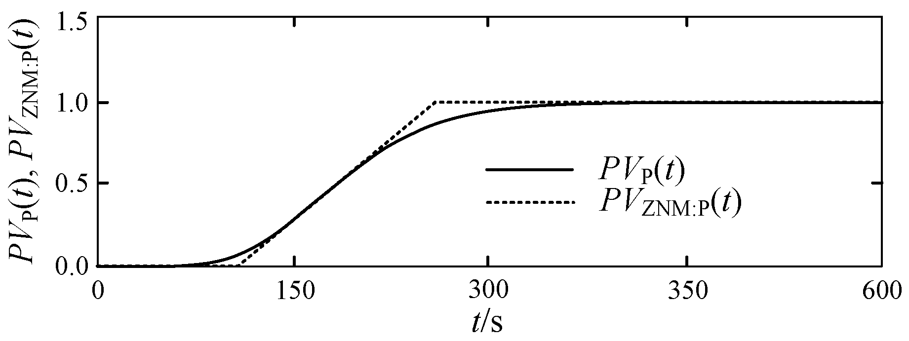
The ZNM principle is a self-balancing process, with the maximum slope point of the rise in the open-loop response curve of the 10th-order process. If all lines fit this maximum slope, according to the tangent and the two intersection points of the start value and the end value (horizontal line), the ZNM process that fits the 10th-order process outputs , as shown in Figure 4 [13].
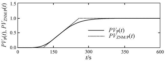
Figure 4.
Schematic diagram of ZNM process output.
The ZNM is used for EFC parameter tuning:
where is the parameter adjustment item.
According to Equations (7) and (8), is taken. The EFC parameters are obtained as , , and . The simulation results obtained in the process, given as a unit step, are shown in Figure 5.
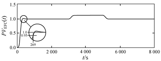
Figure 5.
Schematic diagram of EFC control simulation results.
Based on the data presented in Figure 5, the implementation of engineering fastest control (EFC) results in an overshoot of 2.18%, an adjustment time of 269 s, and a maximum deviation of 0.132, as observed during the RF period. It is evident that this parameter tuning method for EFC yields superior control performance.
However, it is important to note that this EFC parameter tuning method primarily stems from practical engineering experience and is supported by extensive empirical evidence. Developing a theoretical framework from this parameter tuning method poses considerable difficulty.
4. Simulation and Result Analysis
4.1. Simulation Control System
We define the simulation control system (SCS) as shown in Figure 6.
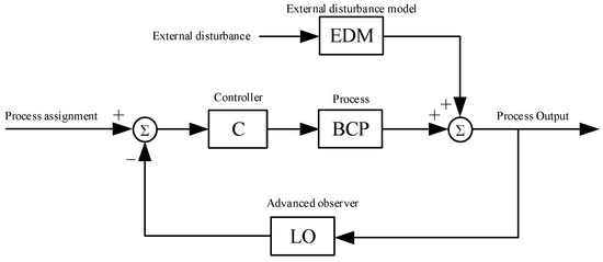
Figure 6.
Schematic diagram of the simulation control system.
The controller (C) includes PI, EFPI, etc. the leading observer (LO) includes PD, the EFLO, etc. External disturbance through the external disturbance model (EDM) is directly coupled to the process output of the being control process (BCP). The ramp function (RF) is used for external disturbance, where the RF rate is and the RF length is 2000 s. The reason for the use of the RF in external disturbance is that the process disturbance of thermal power units generally has the nature of an RF.
We define the BCP and EDM as
where is the transfer function of the BCP and is the transfer function of the EDM.
4.2. Comparison of the Upper-Limit Control Performance of the Engineering Speed Controller and the PID Controller
The determination of the linear higher-order process and controller sets the theoretical upper limit for the control performance of a system. This upper limit represents the highest achievable control performance under critical stability conditions, beyond which further improvement is not possible. It is worth noting that studying the upper limit of performance for EFC or PID control alone has limited significance. However, comparing the upper-limit control performance between EFC and PID control can provide valuable insights and help to address the problem at hand.
Critical stability, as defined in reference [18], is a general concept that encompasses an amplitude stability margin in decibels (dB) and a phase stability margin. Analyzing the stability boundary of a control system is an important aspect of this concept. The critical stability parameter search presented in this study represents a form of stability boundary analysis, albeit with different expressions.
Regarding the PID, EFC, PID open-loop system (PID:OLS), the frequency domain function is
where and are, respectively, PID’s and EFC’s open-loop system frequency domain function. , , , , and are PI, the BCP, PD, the EFPI, and the EFLO.
The stability margin of the open-loop system is
where , , and are the frequency domain function, amplitude-frequency gain, and phase frequency of the open-loop system. and are, respectively, the phase margin and amplitude margin of the open-loop system.
and are, respectively, used to express the amplitude-frequency gain of the open-loop system of PID and EFC. and are, respectively, used to express the phase frequency of PID and EFC open-loop systems.
At critical stability, the phase margin of the open-loop system is , the amplitude margin is 0 dB, and the , , and of EFC are obtained as multiple sets of curves, as shown in Figure 7. Furthermore, it is worth noting that all the simulations in this study were implemented using Microsoft Visual C++ 6.0, a specialized tool developed by the author.

Figure 7.
The diagram of search results of critical stability parameters of EFC.
As shown in Figure 7, a set of curves with the minimum value of is selected from multiple sets of curves representing the upper limit of the control performance of EFC under critical stability, and the critical stability parameters of EFC are obtained. The acquisition of PID critical stability parameters, including EFC and PID stability parameters, is similar.
For comparison, where TEFLO = 180s and in EFC, the minimum value of is 86.75s, corresponding to KEFPI = 2.704. In the case of PID at , the minimum value of is 79.70s, corresponding to . The and change curves of EFC and the and change curves of PID are obtained, as shown in Figure 8.

Figure 8.
The diagram of search results of critical stability parameters of PID and EFC.

Table 1.
EFC and PID parameters of group A.
According to the EFC and PID parameters of group A, and are obtained, as shown in Figure 9.
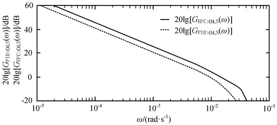
Figure 9.
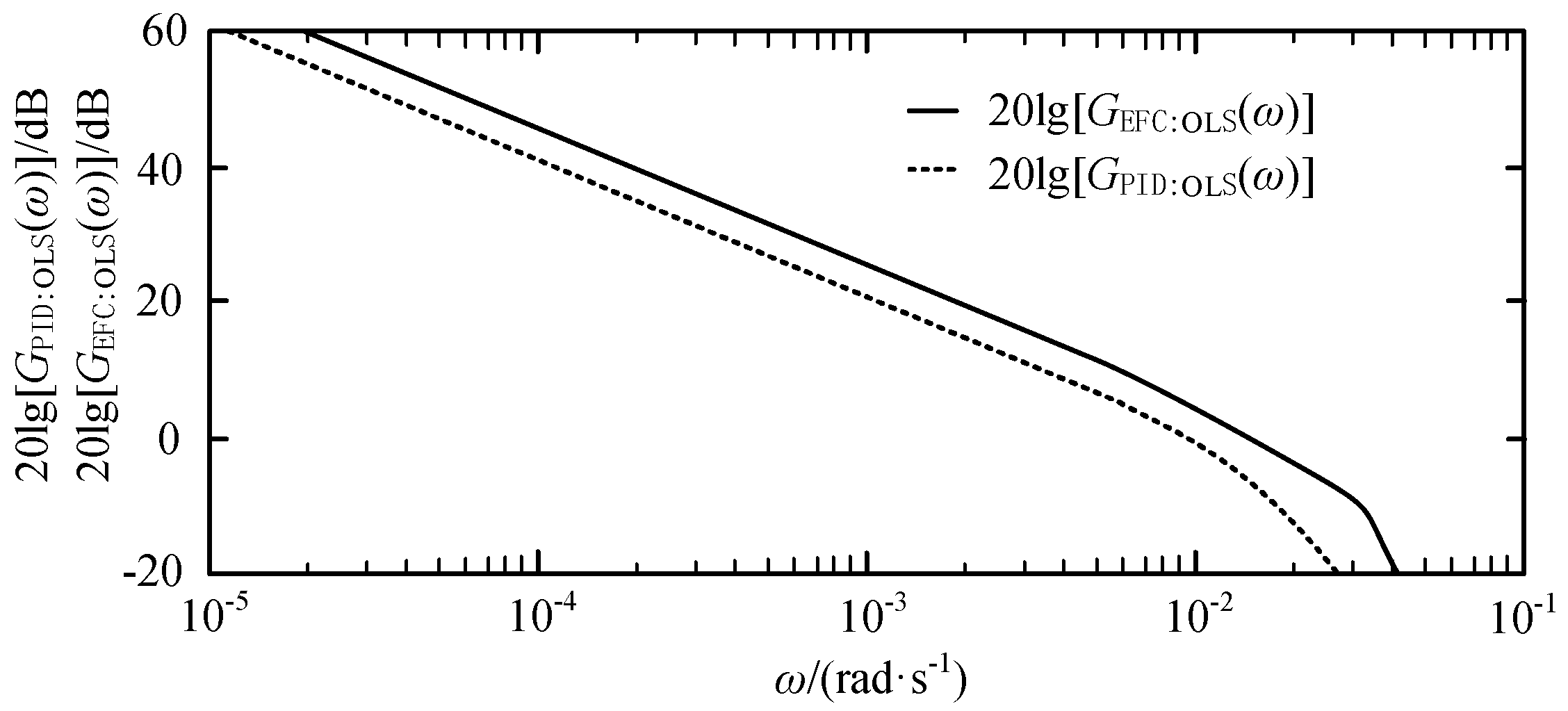
The diagram of frequency-domain gain of open-loop system of PID and EFC.
The results given in Figure 9 represent the upper limit of the control performance of EFC and PID at critical stability. In order to control the upper limit of the performance comparison, the relative zero frequency gain (RZFG) is used to measure the improvement of the upper limit of the control performance of the EFC-phase PID.
According to the EFC and PID parameters of group A given in Table 1, the comparison results are as follows:
where is the RZFG of EFC relative to PID and the RZFG of EFC is 1.7291 times that of PID, which represents a mathematical basis. Based on this mathematical basis, the basic conclusion is that EFC breaks through the upper limit of PID control performance.
4.3. Simulation Comparison of Stable Control Performance
In practical control engineering, proportional–integral (PI) control is widely utilized due to its simplicity, requiring only two parameters. As a point of reference, this section includes a comparison of the performance of PI control.
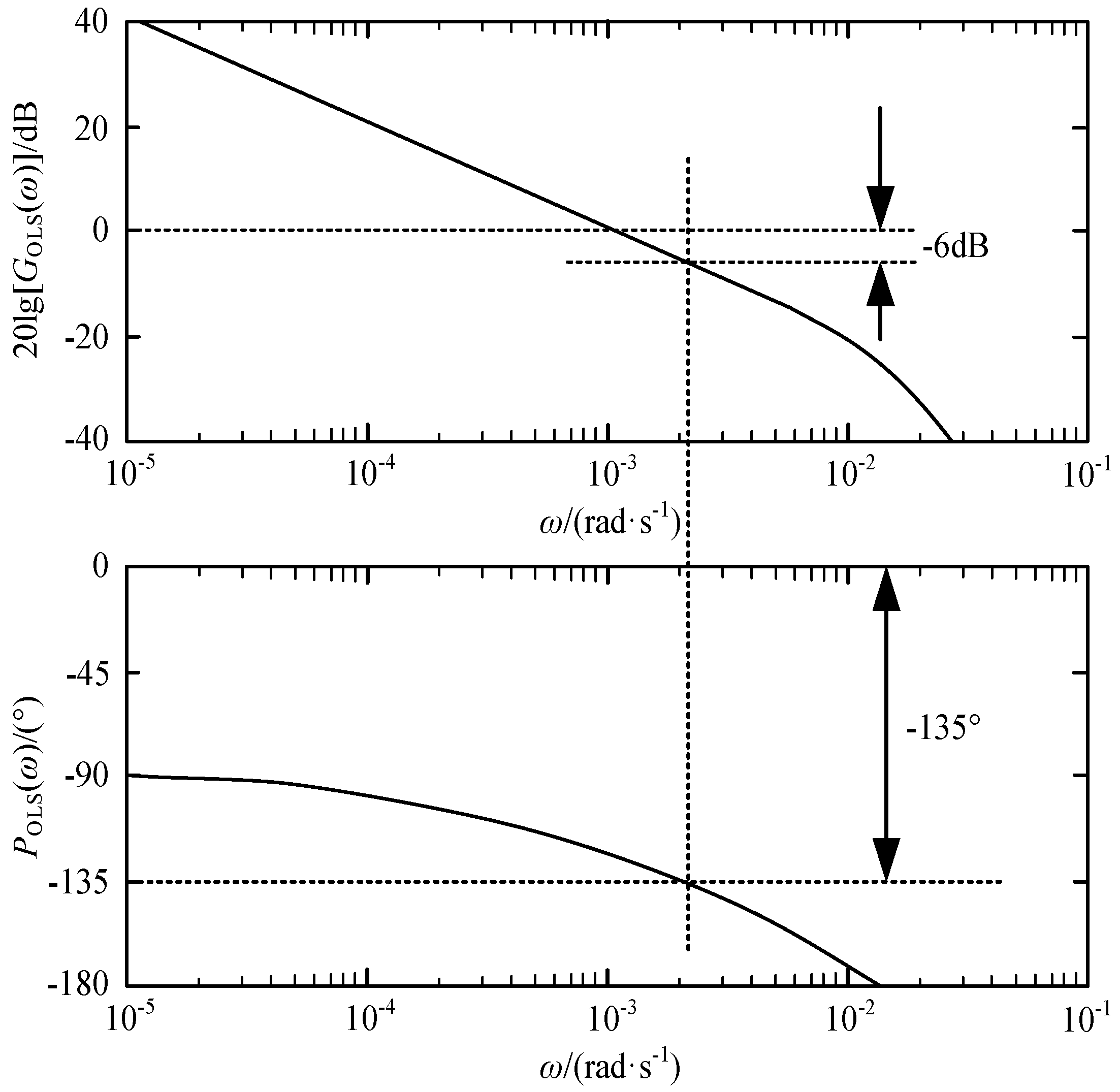
However, it is important to note that the upper limit of control performance under critical stability conditions holds limited significance in real-world projects. The stability performance within the upper limit is not the sole consideration. When comparing the stability performance of engineering fastest control (EFC) and PID control, careful consideration must be given. For instance, the amplitude margins may differ even when the phase margins are the same, and vice versa. To address this issue, the concept of a relative stability margin is introduced. Specifically, in Figure 10, when the amplitude-frequency gain of the open-loop system is −6 dB and the phase frequency is −135°, the relative stability margin is determined.

Figure 10.
The diagram of parameter search condition of EFC and PID.
The advantage of using the relative stability margin is that it has good robustness, such as when the gain mismatch in the control process is increased by two times the phase margin of the open-loop system, which can still be guaranteed to be 45°.
Corresponding to KEFPI = 0.8052, when TEFLO = 235s in EFC, the minimum value of is 383.6s. Corresponding to KP = 0.396, in the of the PID, the minimum value of is 322.5s. Corresponding to , the minimum value of for PI is 429.10s. The search results for EFC, PID, and PI parameters are obtained, as shown in Figure 11.
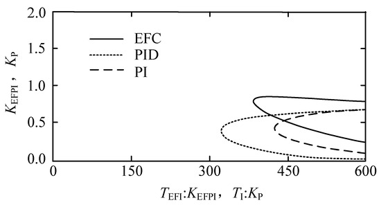
Figure 11.
The diagram of search results of parameters of NFC, PID, and PI.
According to Figure 11, the EFC, PID, and PI parameters of group B are obtained, as shown in Table 2.
Table 2.
Group B parameters of EFC and PID.
According to the EFC and PID parameters of group B, the process is given as a unit step. The RF is added at to obtain the process output controlled by EFC, the process output controlled by PID, and the PI-controlled process outputs , as shown in Figure 12.
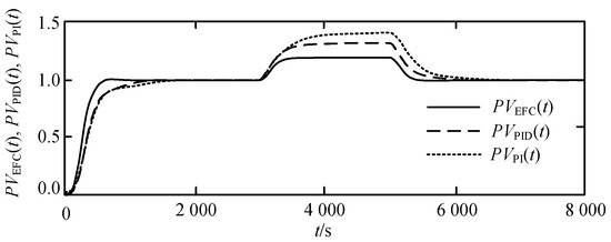
Figure 12.
The diagram of simulation experimental results of control characteristics of EFC, PID, and PI.
According to Figure 12, the main performance indicators of EFC, PID, and PI control are obtained, as shown in Table 3.
Table 3.
Main performance index of control of EFC and PID.
The adjustment time is the time when the process enters to a deviation of less than 5%. Compared with the regulation performance of PI, the regulation performance of PID is increased by 24.7% and the regulation performance of EFC is increased by 96.9%. Compared with the regulation performance of PID, the regulation performance of EFC is improved by 57.9%.
According to Figure 12, the main performance indexes of EFC, PID, and PI control are obtained, as shown in Table 4.
Table 4.
Main performance index of disturbance rejection of EFC, PID, and PI.
Indeed, using the suppression of the maximum deviation in the reference value (RF) as a measure of the disturbance rejection performance of EFC, PID, and PI controllers provides a clear and intuitive assessment. The rationale behind this is that once the disturbance on the process stabilizes, the maximum deviation between the process output and the setpoint can be used to fully evaluate the relative performance of the two controllers in terms of disturbance rejection. This measure offers a practical and straightforward way to compare and assess the effectiveness of different control strategies in mitigating external disturbances. Compared with PI, the external interference rejection performance of PID is improved by 32.6% and EFC’s external disturbance rejection performance is improved by 115.7%. Compared with PID, the external disturbance rejection performance of EFC is improved by 62.2%.
5. Engineering Application of EFC in Fired Thermal Power Units
5.1. Flue Gas Baffle Control of Reheating Steam Temperature of Thermal Power Unit Boiler
In the early stages following the invention of engineering fastest control (EFC), it found widespread application in addressing longstanding control challenges in thermal power units, particularly in the context of flue gas baffle control (FGBC) for the reheating steam temperature in boilers [13]. FGBC had been a difficult problem to solve, with the main obstacle being the inability to achieve automatic control. This was also the prevailing situation for the majority of thermal power units in China.
FGBC offers significant economic advantages, but its lack of automatic control capability hindered its implementation. On the other hand, desuperheating water spray control is easier to automate but suffers from poor economic performance. For instance, increasing the rated feed water flow rate of the boiler by 1% leads to a reduction in boiler thermal efficiency of approximately 0.2%.
Engineers have long pursued various control methods in their efforts to achieve automatic FGBC. These include optimal PID control [19], model predictive control (MPC) [20], dynamic matrix control (DMC) [21], internal model control (IMC) [22], and Smith estimated control [23]. However, achieving automatic FGBC has remained a persistent challenge. As a result, the desuperheating water spray control mode has been predominantly used, significantly impacting the operational efficiency of thermal power units.
To address the issue of automatic control in FGBC, EFC was applied to optimize the FGBC system of a 1000 MW ultra-supercritical thermal power unit boiler, as depicted in Figure 13.
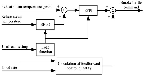
Figure 13.
The optimization diagram of FGBC system.
Figure 13 illustrates the utilization of the load function [15] to adjust the parameters of engineering fastest proportional–integral (EFPI) and the engineering fastest load observer (EFLO) based on the load set for the unit. The EFPI parameters exhibit favorable tracking capabilities for variations in process characteristics. Additionally, the feedforward control quantity is calculated to determine the amount of feedforward control [24] based on changes in the set load and load rate of the unit.
Among them, under loads of 480 MW and 840 MW, the approximate characteristics of the control process are as follows:
where and are, respectively, controlled in the process under a load of 480 MW and the approximate transfer function at 840 MW.
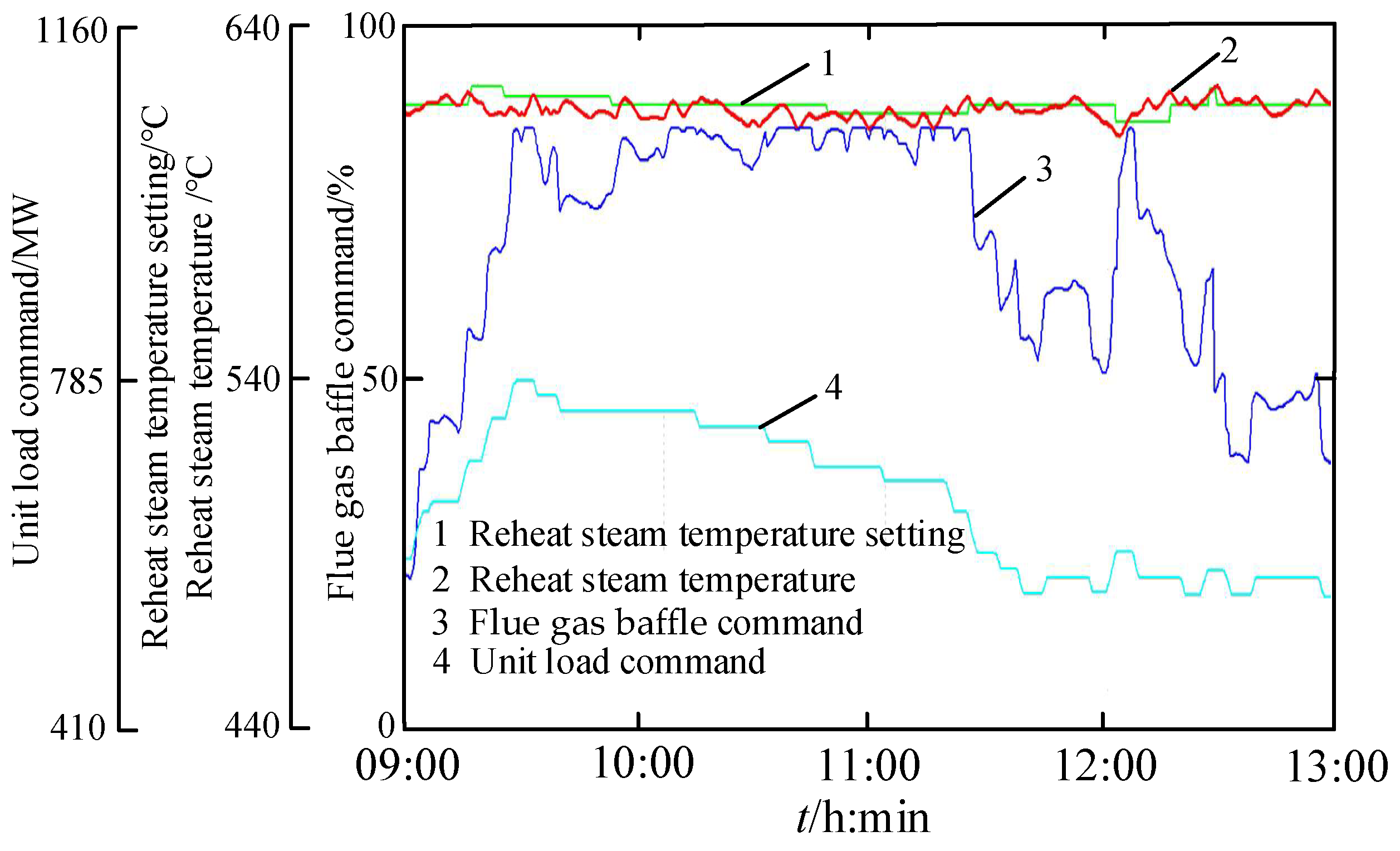
After the FGBC system is optimized by EFC, the 4 h operation trend chart is shown in Figure 14.
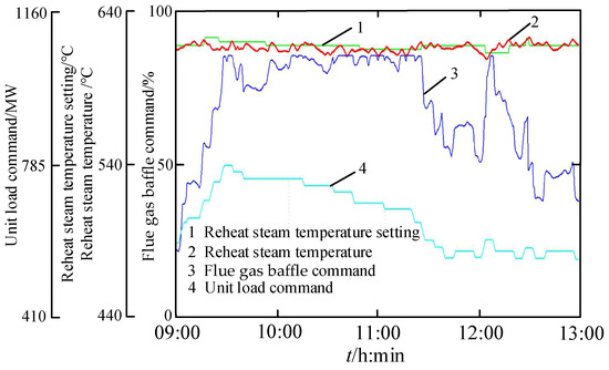
Figure 14.
The diagram of control properties of flue gas baffle control after optimization.
Figure 14 shows that the maximum deviation of the reheating steam temperature from the set value is for the given trend range +3.4 °C/−8.9 °C, which fully meets the requirements of thermal power unit operation regulations. EFC’s long-term application effect is good.
5.2. NOx Reduction Control of Coal-Fired Thermal Power Units
The NOx reduction system in coal-fired thermal power units plays a crucial role in removing nitrogen oxides (NOx) from the flue gas generated by boilers. However, controlling the NOx reduction system presents significant challenges. In January 2022, engineering fastest proportional–integral (EFPI) control was implemented to optimize the control of the NOx reduction system in a 1000 MW coal-fired thermal power unit.
Typically, the control strategy for NOx reduction involves a combination of feedforward control and proportional–integral (PI) feedback correction. The feedforward control is primarily used to maintain a constant value control. However, during steady-state conditions, the feedforward control alone may not be effective. In such cases, the PI feedback correction is employed to eliminate any steady-state bias in the NOx reduction process. This feedback correction helps to ensure that the system operates with minimal deviation from the desired NOx reduction targets.
We replace PI with EFC, as shown in Figure 15.
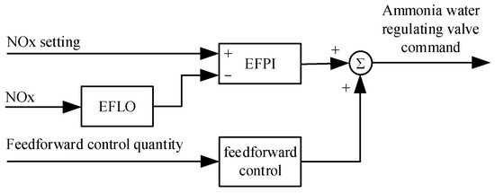
Figure 15.
The optimization diagram of NOx reduction control system.
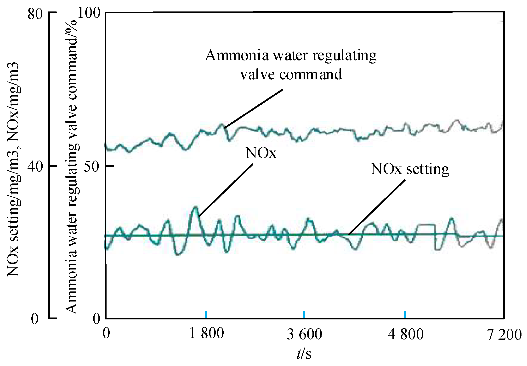
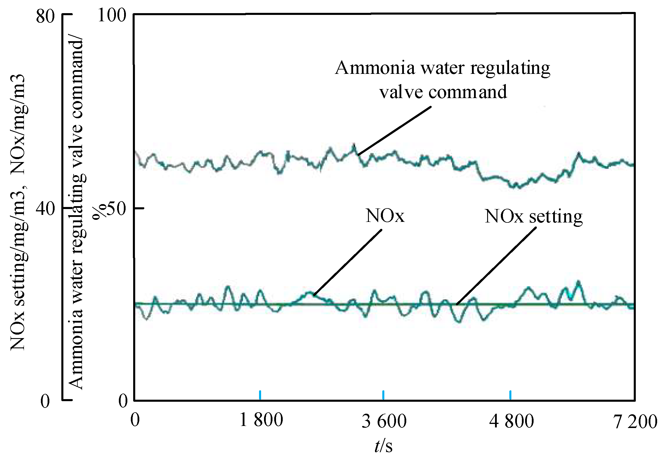
Before using EFC optimization, the PI control trend under steady-state conditions is shown in Figure 16.

Figure 16.
The control properties of NOx reduction control system before optimization.
As shown in Figure 16 of the ammonia–water regulating valve command, within the given trend range, the peak value of the NOx process is 14.8 mg/m3.
After using EFC optimization, the trend of EFC control under steady-state conditions is shown in Figure 17.
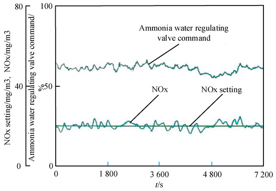
Figure 17.
The control properties of NOx reduction control system after optimization.
As shown in Figure 17, after using EFC optimization, the peak NOx process value is 9.7 mg/m3 within the given trend range. It can be seen that using EFC optimization achieves significant results.
In the actual process control of thermal power units, the steady-state deviation is not a smooth curve that tends to a certain end value, but a random curve that fluctuates around the set value. Compared to PI, the fluctuation range using EFC is relatively low. From an engineering perspective, the performance of EFC has been verified.
6. Conclusions
Based on the research conducted in this study, the following conclusions can be drawn:
- (1)
- Based on simulation results, the proposed engineering fastest control (EFC) model in this study demonstrates advantages such as a fast convergence speed, good disturbance rejection performance, and ease of parameter tuning. It significantly improves the rapid frequency regulation performance of existing power plant units, meeting the needs of renewable energy control requirements.
- (2)
- Through this research, it is evident that the engineering fastest tracking filter (EFTF) is a linear filtering technique with excellent filtering characteristics. It can be applied in signal filtering and other processing tasks, as well as in control domains such as integral–differential controller structures and novel feedback control architectures.
- (3)
- EFTF and EFC are products of control engineering practice which represent original innovations in filtering and control mechanisms. They are significant developments in the field of control engineering, contributing to its advancement.
Author Contributions
Conceptualization, S.S. and P.C.; methodology, S.S. and J.L. (Jun Li); validation, Z.W. and L.L.; formal analysis, Z.L. and J.L. (Jun Li); writing—original draft preparation, J.L. (Jiahao Liu) and L.L.; writing—review and editing, S.S. and J.C.; project administration, S.S. and J.L. (Jun Li); funding acquisition, P.C. and S.S. All authors have read and agreed to the published version of the manuscript.
Funding
This research was funded by the by the key research and development program of Shanxi Province (grant no. 202202020101001); the National Natural Science Foundation of China (grant no. 62003314); and the Fundamental Research Program of Shanxi Province (grant no. 202103021224187, 20210302124010, and 20210302123050).
Data Availability Statement
The data presented in this study are available on request from the corresponding author. The data are not publicly available due to privacy.
Conflicts of Interest
Author Jun Li was employed by the company Electric Power Research Institute of Guangdong Power Grid Co., Ltd. The remaining authors declare that the research was conducted in the absence of any commercial or financial relationships that could be construed as a potential conflict of interest.
References
- Yang, M.; Duan, L.; Tong, Y. Design and Performance Analysis of New Ultra-Supercritical Double Reheat Coal-Fired Power Generation Systems. Energies 2021, 14, 238. [Google Scholar] [CrossRef]
- Allison, T.C. STEP Advances Supercritical CO2 Power Cycles for Gas-Fired Generation. Pipeline Gas J. 2021, 248, 22–26. [Google Scholar]
- Villeneuve, Y.; Séguin, S.; Chehri, A. AI-Based Scheduling Models, Optimization, and Prediction for Hydropower Generation: Opportunities, Issues, and Future Directions. Energies 2023, 16, 3335. [Google Scholar] [CrossRef]
- Tsai, Y.-C.; Yang, C.-W. Unfiltered air inleakage analysis of the control room envelope of Kuosheng nuclear power plant. Kerntechnik 2023, 88, 604–614. [Google Scholar] [CrossRef]
- Zhang, J.; Li, H.; Cheng, P.; Yan, J. Interpretable Wind Power Short-Term Power Prediction Model Using Deep Graph Attention Network. Energies 2024, 17, 384. [Google Scholar] [CrossRef]
- Anselmo, S.; Ferrara, M. Trends and Evolution of the GIS-Based Photovoltaic Potential Calculation. Energies 2023, 16, 7760. [Google Scholar] [CrossRef]
- Sodri, A.; Septriana, F.E. Biogas Power Generation from Palm Oil Mill Effluent (POME): Techno-Economic and Environmental Impact Evaluation. Energies 2022, 15, 7265. [Google Scholar] [CrossRef]
- Wu, Y.; Xu, C.; Xu, H. Optimal Site Selection of Tidal Power Plants Using a Novel Method: A Case in China. Energies 2016, 9, 832. [Google Scholar] [CrossRef]
- Tong, L. Research on stability of hydraulic system based on nonlinear PID control. Nonlinear Eng. 2022, 11, 494–499. [Google Scholar]
- Wang, W.-Z.; Wu, Z.-W.; Chai, T.-Y. PID Control with Output Compensation for the Fused Magnesia Smelting Process. Acta Autom. Sin. 2018, 44, 1282–1292. [Google Scholar]
- Su, J.; Zeng, Z.H. Auto-coupling PID control method for nonlinear time varying systems. Control. Theory Technol. 2022, 39, 299–306. [Google Scholar]
- He, J.; Xiao, M.; Lu, Y.; Wang, Z.; Zheng, W.X. Fractional-order PID control of tipping in network congestion. Int. J. Syst. Sci. 2023, 54, 1873–1891. [Google Scholar] [CrossRef]
- Li, J.; Huang, W.J.; Chen, J.P.; Wang, P.; Zhou, Y.Y.; Zhu, Y.Q.; Pan, F.P.; Li, D.B. An Engineering Fastest Controller Adaptive to Deep Peak and Fast Frequency Regulation for New Power System. Guangdong Electr. Power 2021, 34, 110–119. [Google Scholar]
- Li, J.; Huang, W.J.; Chen, J.P.; Wang, P.; Zhou, Y.Y.; Zhu, Y.Q.; Pan, F.P.; Li, D.B. An Accelerated Engineering Fastest Proportional Integral Controller to Meet the Needs of the Development of New Power System. Guangdong Electr. Power 2022, 35, 170–178. [Google Scholar]
- Li, J.; Huang, W.; Wan, W.; Liu, Z. Research and application of a novel feedback controller. Control. Theory Appl. 2020, 37, 411–422. [Google Scholar]
- Hui, N.; Feng, Y.; Han, X. DC offset elimination method of Phase-locked loop based on novel generalized integrator. Energy Rep. 2021, 7 (Suppl. S1), 30–35. [Google Scholar] [CrossRef]
- Gai, R.; Chen, G. On Constrained MMVC of Discrete-Time First-Order Linear Stochastic Systems with PSI I: The Critically Stable Case. Asian J. Control. 2014, 17, 932–941. [Google Scholar] [CrossRef]
- Ziegler, J.G.; Nichols, N.B. Optimum Settings for Automatic Controllers. J. Fluids Eng. 1942, 64, 759–765. [Google Scholar] [CrossRef]
- Aafaque, M.; Boker, A.; Sardahi, Y. Three-time scale multi-objective optimal PID control with filter design. Asian J. Control. 2023, 25, 3356–3368. [Google Scholar] [CrossRef]
- Li, L.; Hu, L.; Su, R.; Ruan, X.; Fu, X.; Sun, Z.; Zhu, C. Nonlinear disturbance observer-based model predictive control for magnetically levitated slice motor. Nonlinear Dyn. 2023, 111, 21797–21814. [Google Scholar] [CrossRef]
- Huang, J.; Wang, Y.; Yang, S.-H.; Xu, Q. Robust stability conditions for remote SISO DMC controller in networked control systems. J. Process Control 2009, 19, 743–750. [Google Scholar] [CrossRef]
- Yao, J.; Liu, X. Fuzzy Multi-model Internal Model Control for the Secondary Last Temperature of Low-pressure Cylinder Zero Output Operation. Electr. Power Sci. Eng. 2022, 38, 61–69. [Google Scholar]
- Guo, X.; Shirkhani, M.; Ahmed, A.M. Machine-Learning-Based Improved Smith Predictive Control for MIMO Processes. Mathematics 2022, 10, 3696. [Google Scholar] [CrossRef]
- Liu, B.; Song, Z.; Yu, B.; Yang, G.; Liu, J. A Feedforward Control-Based Power Decoupling Strategy for Grid-Forming Grid-Connected Inverters. Energies 2024, 17, 424. [Google Scholar] [CrossRef]


Disclaimer/Publisher’s Note: The statements, opinions and data contained in all publications are solely those of the individual author(s) and contributor(s) and not of MDPI and/or the editor(s). MDPI and/or the editor(s) disclaim responsibility for any injury to people or property resulting from any ideas, methods, instructions or products referred to in the content. |
© 2024 by the authors. Licensee MDPI, Basel, Switzerland. This article is an open access article distributed under the terms and conditions of the Creative Commons Attribution (CC BY) license (https://creativecommons.org/licenses/by/4.0/).