Abstract
Agricultural emissions can be significantly reduced with smart farming, which includes moving away from large conventional tractors to fleets of compact wheeled electric robots. This paper presents a novel simulation modeling approach for an ATV-sized wheeled electric agricultural robot pulling an implement on deformable terrain. The 2D model features a semiempirical tire–soil interaction model as well as a powertrain model. Rear-wheel drive (RWD), front-wheel drive (FWD), and all-wheel drive (AWD) versions were developed. Simulations were carried out on two different soils to examine the energy consumption and tractive performance of the powertrain options. The results showed that energy consumption varies the least with AWD. However, RWD could provide lower energy consumption than AWD with light workloads due to lower curb weight. However, with the heaviest workload, AWD had 7.5% lower energy consumption than RWD. FWD was also found to be capable of lower energy consumption than AWD on light workloads, but it was unsuited for heavy workloads due to traction limitations. Overall, the results demonstrated the importance of taking the terrain characteristics and workload into account when designing electric agricultural robots. The developed modeling approach can prove useful for designing such machines and their fleet management.
1. Introduction
The world population is projected to reach 9.7 billion by 2050 [1]. Thus, the demand for food is expected to rise considerably, necessitating advancements in agricultural productivity [2]. Simultaneously, agriculture, a significant contributor to greenhouse gas (GHG) emissions and environmental degradation, must also adapt to mitigate its environmental impact [3]. It has been estimated that agriculture accounts for approximately 10% of the European Union’s total GHG emissions [4]. Globally, the agricultural sector is responsible for approximately 15% of all GHG emissions [5]. Thus, there is an urgent need to find ways to optimize agricultural operations and food production in order to reduce the carbon footprint of farm machinery. Using biofuel blends has been suggested as one solution for reducing the emissions of agriculture [6]. However, achieving significant emission reductions will require more fundamental changes. The electrification of agricultural machinery presents a promising pathway towards achieving the dual objectives of increased productivity and environmental sustainability.
The concept of smart farming, which involves the utilization of technologies such as the Internet of Things, artificial intelligence, and robotics to increase the efficiency of agricultural operations, has received significant research interest in recent times [7]. The electrification of agricultural machines and the utilization of renewable energy sources are known to be essential steps towards the widespread implementation of smart farming [2]. Consequently, studies focusing on using renewable energy in agriculture have greatly increased in recent years [8]. However, the high energy demand of agricultural operations makes the electrification of the machinery challenging [9]. The issues with battery electric agricultural machinery are compounded by the costs, slow charging, and lack of existing charging infrastructure [10,11]. Nonetheless, recent studies have shown that electrification of on-field operations can be a techno-economically feasible option for reducing emissions caused by the agricultural sector [12,13,14,15]. Depending on the type of farm, the carbon footprint of a farm can be reduced by up to 70% with electrification in an appropriate process with renewable energy resources [16].
Yet, various challenges remain on the path towards widespread implementation of electrified farm machinery. The currently available electric machinery is only suitable to a small niche of farm types [17]. It has been shown that the ability to operate autonomously will be essential for wheeled electric agricultural robots to achieve working rates comparable to conventional diesel systems [13]. Recent advancements in machine vision technology have significantly increased the viability of autonomous operation in farm environments [18]. Furthermore, one solution to the range limitations of battery electric agricultural machinery is to utilize a fleet of smaller autonomous robots [13]. The viability of autonomous battery electric robot fleets can be further enhanced by integrating on-site renewable energy generation and storage [15]. The continuing improvements in photovoltaic (PV) solar energy conversion technology can make agrivoltaics a particularly potent aspect of future smart farming solutions [19]. The integration of PV modules to autonomous agricultural robots may also further improve their viability [20]. However, it has also been shown that the optimal design parameters of autonomous agricultural robots significantly depend on the environment the robot will operate in [21]. It is also worth noting that moving away from conventional large and heavy tractors to fleets of compact, light machines has the added benefit of mitigating issues with soil compaction [22,23]. Operating heavy tractors on farmlands reduces the hydraulic conductivity and water storage capacity of subsoils, which results in reduced yields.
However, despite the increased research focus on battery electric agricultural machinery, only limited attention has been given to developing comprehensive accurate simulation models specifically tailored for electric agricultural machinery, including operating different agricultural implements. Detailed simulation models that simulate all the components of the machines that are critical to their viability and energy efficiency will be crucial for optimizing the operation of the machines. To that end, this research presents a novel approach to modeling a compact all-terrain vehicle (ATV)-sized battery electric wheeled agricultural robot pulling an implement. The simulation model includes powertrain, tire–soil interaction, and implement models. The tire–soil model includes a deformable terrain. The modeling approach was utilized to create a simulation model of a generic electric agricultural robot pulling a tine harrow to facilitate a comparison between different robot designs and their effectiveness on different soils and operation cycles. The energy consumption of different powertrain configurations, including rear-wheel drive (RWD), front-wheel drive (FWD), and all-wheel drive (AWD), are compared on different soil types. The results provide novel insights into the advantages and disadvantages of alternate powertrain configurations on different soils. The results will also provide a better understanding of how the configuration of the farm implement and the consequent changes in the draft force affect the energy consumption with different powertrain configurations and soils. In addition, the results will demonstrate the effect the weight distribution of the vehicle has on the energy consumption.
In this article, we begin with a literature review of tire–soil interaction modeling and simulations of agricultural machinery. In Section 3, the simulation model of the agricultural robot is presented. The simulation results are then presented and discussed in Section 4. In the final Section 5, conclusions are drawn based on the findings, and future developments are considered.
2. Modeling of Tire Soil–Interaction and Agricultural Machinery: State of the Art
2.1. Tire–Soil Interaction Models
The main objective of modeling the tire–soil interaction is to be able to accurately calculate the force and moment characteristics of tires on deformable terrain [24]. Another objective, which is particularly important in agricultural studies, is to assess the effect tire passage has on the properties of the soil such as soil height and compaction. Tire–soil interaction models can be divided into three categories: empirical, semiempirical, and physics-based models [25]. Empirical models were initially popular, but later on, the research focus shifted more towards semiempirical models. In recent years, physics-based models have become a topic of high research interest.
Empirical models are constructed in three steps [25]. The first step is to identify the most influential measurable factors on vehicle performance. Then, wheel mobility experiments are conducted. In the last step, curve-fitting methods are used to capture trends in the measured data. One widely used empirical factor is the vehicle mobility number, which is a function of soil strength, tire load, and tire geometry. A classical example of an empirical tire–soil interaction model is the VCI model developed by the US Army Corps of Engineers Waterways Experiment station (WES) in the 1970s [26]. The model calculates the mobility index based on measured data using a series of empirical equations. If the index does not exceed the cone index of the soil, mobility on the terrain is then not considered possible. The WES also developed a mobility numeric model, which calculates the ratio of soil strength to a nominal unit load the tire applies to the soil. The model was further revised in a later study [27]. Similar approaches to the WES were taken in later studies [28,29,30]. Another empirical approach was taken by Schreiber and Kutzbach, who devised a traction prediction model by analyzing a large quantity of measured traction curves and identifying the most important factors affecting the tractive performance [31].
Unlike purely empirical tire–soil interaction models, semiempirical models utilize not only experimental measurements and empirical formulas but also analytical methods; while various semiempirical models have been developed over the years, the most widely used model is the formulation devised by Bekker and Wong [32,33,34,35]. The model represents the normal and shear stresses in the contact patch as functions of the tire kinetics and soil characteristic parameters. The stresses are then integrated over the contact patch to calculate the tire forces, driving torque, and soil deformation. Over the years, various modified versions of the model have been developed. Sandu et al. modified Bekker’s normal stress formulation to include the effect of variations in soil moisture [36]. Mao and Han developed nonlinear complementarity equations for the model that were shown to improve its accuracy [37]. Senatore and Sandu developed their own version of the Bekker–Wong model that included the multipass effect [38]. They additionally utilized the developed model to analyze the influence of torque distribution on tractive efficiency and mobility [39]. Cheng and Lu compared different methods for determining parameters for a tire–soil interaction model based on Bekker’s equations [40]. Jiang et al. devised numerical models to quantify Bekker’s soil characteristic parameters for paddy soils using data acquired from soil bin tests [41]. The Bekker–Wong model has been utilized for various purposes in past studies. Holtz et al. used the model as part of a multibody vehicle model to investigate rollovers on sloped terrains [42]. Krenn and Hirzinger used the Bekker–Wong model as the basis of their soil contact model (SCM), which provides an interface for the tire–soil interaction model and a 3D multibody system simulation [43]. The SCM was utilized to simulate the locomotion of a Mars rover [44]. An extended version of the SCM is available in the open-source multiphysics package Chrono [45,46,47]. In recent times, the Chrono implementation of the SCM has been utilized for researching teaching artificial intelligence to control vehicles on deformable terrains [48,49]. The AESCO soft soil tire model (AS2TM) also utilizes Bekker’s equations as the basis for simulating both rigid and flexible tires on deformable terrains [50]. Recently, Karpman et al. presented a novel approach of augmenting a tire–soil model based on Bekker’s equations with a neural network to better capture the dynamic nature of soil reaction forces [51]. Other approaches have also been taken for semiempirical modeling of tire–soil interaction. The widely used FTire model divides the tire into multiple flexible ring elements to form a three-dimensional model, which can also simulate the relation between the contact pressure and tire sinkage [52]. Roşca et al. created a semiempirical traction performance prediction model for tractors, which was based on the assumption that the shape of the tire–soil contact patch is a superellipse [53]. Pavlov and Johnson developed a synthesized semiempirical tire model with a focus on making the model operate realistically even at high slip angles and slip ratios [54].
Physics-based tire–soil interaction models utilize physical principles and analytical methods to represent tire and terrain structures and their interaction [25]. Although such approaches enable high-fidelity simulation of the tire–soil contact, the main disadvantage of the physics-based methods is that they tend to have high computational time requirements. The two primary physics-based method categories are finite element methods (FEMs) and particle-based methods, such as smoothed particle hydrodynamics (SPH) and the discrete element method (DEM) [55]. Earlier FEM tire models were typically only two-dimensional [56,57,58]. However, with increases in computational power available, 3D FEM models have become more commonplace [59,60,61,62,63]. FEM-based tire–soil interaction models are available in several commercial products such as ABAQUS [64], LS-DYNA [65], and MARC [66] as well as in the aforementioned open-source Chrono [45]. One commonly used physics-based approach is to utilize a finite element model for the tire and a granular discrete element model for the soil [57,59,61,62]. Granular soil models have also been shown to work well with a more simple tire model that considers the tire to be a rigid body [67].
Although SPH is one of the most mature particle-based methods for solving computational mechanics problems, its use in terramechanics is a recent development [55]. SPH can be more accurate than FEM-based approaches for simulating soil penetration and soil flow under the tire. Hu et al. introduced an SPH-based method for modeling a deformable soil that a rover with rigid wheels traverses on [68]. The model was utilized to research traction control design for off-road mobility.
2.2. Simulation of Agricultural Machinery
Various previous studies have focused on simulating wheeled agricultural machinery. Conventional internal combustion engine (ICE)-powered tractors have been simulated to study topics such as traction control algorithms [69], drivetrain reliability [70], gear-shifting strategies [71,72], and active suspension [73]. Hybrid powertrains in agricultural tractors have received increased research interest in recent years. The different hybrid powertrain types simulated include a parallel hybrid electric powertrain [74], power-split electric continuous variable transmission (e-CVT) [75], and mechanic–electronic–hydraulic powertrain [76]. Lajunen et al. conducted a comparison of different powertrain topologies for an agricultural tractor using Autonomie software version 2022 [9]. The results showed that a parallel hybrid powertrain can reduce the energy consumption in tillage operations by up to 20% compared to a conventional diesel-engine-based powertrain with light workloads. The consumption reduction is heavily dependent on the workload. On heavy workloads, the reduction can become negligible. However, a fuel cell electric powertrain could reduce the consumption by over 20% and a battery electric powertrain by nearly 60% with heavy workloads. Although different aspects of agricultural tractors have been simulated, it is rare for the models to include a tire–soil interaction model that simulates the deformable soil. Regazzi et al. investigated the effect of key design parameters affecting the power delivery efficiency of an ICE-powered agricultural tractor to quantify their effect on the tractive performance [77]. The 2D simulation model utilized the Bekker tire–soil model. An extended version of the Bekker tire–soil model was also utilized in a recent study focusing on developing a trajectory planning algorithm with slip control for an autonomous mobile agricultural robot [78].
Due to the rapid rate of development of autonomous navigation systems and electric powertrains, autonomous mobile electric agricultural robots have received significant research interest in recent years. Studies have focused both on their viability against conventional ICE tractors [12,13,14] and on navigation [78,79]. Lagnelöv et al. simulated an autonomous battery electric field tractor to investigate different charging systems [10]. In the model, tire losses were modeled with rolling resistance, and the draft force caused by the implement was approximated based on an equation by the American Society of Agricultural Engineers (ASAE) [80]. The study showed that replacing conductive charging with a battery exchange system could reduce the time it would take for a battery electric agricultural tractor to complete operations. However, the results also showed that a battery electric tractor spends significantly more time in transit and recharging compared to an equivalent diesel tractor. In another study utilizing the same simulation model, it was found that employing a fleet of smaller autonomous battery electric tractors would be an effective solution to the battery capacity and recharging issues [13]. Such a fleet could have competitive life-cycle costs compared to conventional ICE tractors due to the lower annual operating costs despite the higher initial investment required. The results of the research also emphasized the importance of autonomy for battery electric compact tractor fleets to achieve working rates comparable to diesel tractors. Utilizing the same simulation model, a study focusing on life-cycle climate impact showed that battery electric tractors could cut the life-cycle GHG emissions to a small fraction of those of diesel tractors when charged with clean electricity [14].
2.3. Research Gap
Tire–soil interaction modeling and simulation modeling of wheeled agricultural machines have been topics of significant research interest for decades. Yet, there is still a distinct lack of high-definition simulation models designed specifically for agricultural machinery. Typically, simulation models of agricultural machines have featured simple tire models with no deformable soil. Models for farm implements have often been omitted entirely. There has also been little focus on examining in more detail the different design factors and soil properties affecting the energy consumption of wheeled electric agricultural robots. Additionally, comparisons between different powertrain configurations for compact wheeled electric agricultural robots have not been conducted.
In this research, the goal was to develop a detailed simulation model of a wheeled electric agricultural robot that would feature a tire–soil interaction model with a deformable terrain, an electric powertrain model, and a model for the dynamics of the implement pulled by the robot. The well-established and extensively used Bekker–Wong tire–soil model was chosen due to its reliability and the amount of data available for it. Implement forces were modeled utilizing the approach developed by Söhne [81]. The novel modeling approach taken could prove useful in the future in the design process of wheeled electric agricultural robots and fleets of such machines. RWD, FWD, and AWD versions of the robot model were created in order to compare the energy efficiency and tractive performance of different powertrain configurations. FWD has been shown to be a potentially viable option for agricultural tractors [82]. Thus, the FWD configuration was included in this study as well. The models were simulated on two different soil types to investigate the effect of the soil properties on the efficiency and tractive performance of the powertrain configurations. The simulation results were extensively analyzed to gain novel insights into the different factors affecting the energy consumption with different powertrain configurations, soils, and implement configurations.
3. Materials and Methods
The two-dimensional simulation model of an ATV-sized compact wheeled electric agricultural robot pulling a tine harrow was developed in MATLAB/Simulink software version R2022b. As was previously mentioned, RWD, FWD, and AWD versions of the model were created. The RWD and FWD versions feature a single electric motor (EM), while the AWD version has a motor on each axle. Each version utilizes a fixed gear ratio. In order to examine the effect of longitudinal weight distribution, two versions were created of the RWD and FWD models. For the RWD model, weight distributions of 40/60 and 30/70 (front/rear) were used. Conversely, the two FWD models featured weight distributions of 60/40 and 70/30. The AWD model had a weight distribution of 50/50.
The main components of the simulation model are the powertrain model, the tire–soil interaction model, the equations of motion of the robot, the harrow dynamics, and the control algorithm. Each of these components will be described in the upcoming subsections. The robot and soil parameters are presented in Section 3.4. Figure 1 and Figure 2 show diagrams of the RWD and AWD models where the different subsystems and the flow of information between them can be seen. A diagram of the FWD version would be identical to the RWD version except the front and rear axles would be switched around. The numbers in the brackets represent the equations utilized by the subsystems. In the figures, v and d represent speed and depth, and the variable x passed from the robot chassis to the harrow subsystem represents a vector of states of the robot, including its longitudinal and vertical positions and speeds as well as the pitch angle and rate. These states are then used by the harrow subsystem to calculate the current states of the harrow.
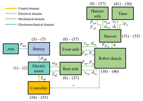
Figure 1.
Diagram of the subsystems and flow of information in the RWD model.
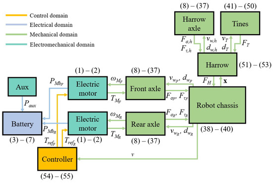
Figure 2.
Diagram of the subsystems and flow of information in the AWD model.
3.1. Powertrain Model
The powertrain model features an efficiency-map-based electric motor model and a resistive battery model. The same modeling approach was taken as in a previous research study focusing on simulating battery electric city buses [83]. In the model, the torque at the driven axle at time t is calculated as
where is the motor torque, is the gear ratio of the final drive, is the efficiency of the final drive, and is the output power of the motor, which is calculated as
where is the rotational speed of the motor.
The motor input power is determined based on the motor output power and efficiency . The output power of the battery is calculated as the sum of and the auxiliary power demand of the electronics and battery pack cooling:
The efficiency of the electric motor depends on the torque and the rotational speed. The efficiency map utilized in the simulations is presented in Section 3.4. The total power consumption of the battery is calculated as a sum of the output power and the internal losses of the battery:
where is the current, is the voltage, and is the internal resistance of the battery, which depends on the state of charge (SOC). The battery current is calculated as
where is the open-circuit voltage of the battery, which is dependent on the SOC. The rate of change of the state of discharge (SOD) of the battery is calculated as
where is the capacity of the battery in Ah. Thus, the SOC can be acquired as
where is the initial SOC of the battery at the start of the simulation. The battery pack parameters are presented in Section 3.4.
3.2. Tire–Soil Interaction Model
The tire model used in the simulation model assumes the tire to be rigid. This assumption was considered to be acceptable due to the relatively small tire size in the simulated robot. The diameter of the robot wheels is 0.635 m, and the harrow wheels have a diameter of 0.584 m. The rigid wheel model used is based on the classic widely used model developed by Wong and Reece [32,33]. A similar tire modeling approach was adopted by Senatore and Sandu in their research focusing on off-road tire modeling and the multipass effect [38]. The tire model is based on calculating the normal and shear stress distributions beneath the tire. The shear stress distribution is calculated utilizing the equation originally defined by Janosi and Hanamoto [84]:
where is the maximum shear stress, j is the terrain shear displacement, k is the shear deformation modulus, and is the angle that describes the angular position of the currently examined tire element. The value of is zero at the bottom of the tire, and the value increases when rotating counterclockwise, as demonstrated in Figure 3.
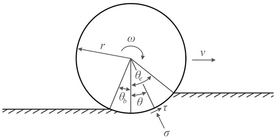
Figure 3.
Normal stress and tangential stress acting on a rigid wheel on deformable soil (adapted from [32]).
The maximum shear stress is calculated according to the Mohr–Coulomb equation:
where c is the soil cohesion, is the normal stress, and is the angle of internal shear resistance of the soil. The definition of the shear displacement depends on the sign of the slip ratio, which is conventionally defined as follows [85,86]:
where is the rotational speed of the wheel, R is the radius of the wheel, and is the longitudinal speed of the wheel. The wheel is slipping when the slip ratio is positive and skidding when it is negative. However, it can be seen in Equation (10) that the slip ratio cannot be calculated for a wheel that has zero longitudinal speed, and at near-zero speeds it can be unstable. Thus, a different formulation was developed to be used at very low speeds. Below a specified threshold speed , the slip ratio is instead calculated as
The model progressively switches to the formulation presented in Equation (10) as the vehicle speed increases. Thus, the full formulation of the slip ratio can be expressed as
where v is the longitudinal speed of the robot and is a speed threshold above which the conventional slip ratio definition given in Equation (10) is used. The threshold speeds were experimentally determined utilizing different soils to find the lowest speeds at which the tire model was found to behave in a stable manner in all conditions. For , the speed was determined as 0.1 km/h, and the value for was set to 2.0 km/h.
For slip (i.e., the wheel has a positive slip ratio), the shear displacement is calculated as follows [32]:
where is the entry angle of the wheel, as seen in Figure 3. As described by Wong and Reece [33], when a wheel is skidding (i.e., it has a negative slip ratio) on a loose surface, there exists a point where the tangential stress changes its direction from opposite to wheel rotation (defined as positive) to the same direction as the wheel rotation (defined as negative). The model accomplishes simulating this phenomenon by accounting for the change in the direction of the shear displacement in the rear region of the tire. An example of the difference in the tangential stress distribution between slipping and skidding is shown in Figure 4. The shear displacement for a skidding wheel is calculated as follows [33]:
where is the angle of maximum stress, and is a supporting coefficient, which is defined as follows [33]:
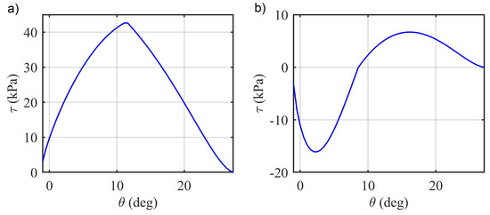
Figure 4.
Tangential (shear) stress as a function of contact angle on sandy loam with a vertical load of 1500 N (a) at a slip ratio of 0.1 and (b) at a slip ratio of −0.1.
The definition of the angle of maximum stress also depends on whether the wheel is slipping or skidding. For slip, it is defined as follows [32]:
where and are empirically estimated constants. For skidding, the angle of maximum stress is defined as follows [33]:
where and are defined as
The normal stress in the contact patch is defined as a piece-wise function. The stress between the leading edge of the contact patch at the angle and the angle at which maximum normal stress occurs ) is defined as follows [38]:
where and are cohesion-dependent and frictional-dependent coefficients specific to the soil material, is the soil bulk density (in N/m3), n is the sinkage index, and b is a parameter related to the contact geometry. The normal stress between the angle and the trailing edge of the contact patch at angle is calculated as follows [38]:
where is the angle of the trailing edge of the contact patch. The sinkage index depends on the slip ratio and is defined as follows [87]:
where and are empirically approximated constants. The geometry-related parameter b is calculated as follows [38]:
where is the projected contact patch length and w is the width of the tire.
The tire forces are then calculated as resultant forces caused by the normal and tangential stress distributions. The longitudinal tire force produced by the normal stress is calculated as follows [32]:
and the vertical force produced by the normal stress is defined as follows [32]:
The longitudinal force produced by the tangential stress can be calculated as follows [32]:
and the vertical force produced by the tangential stress is defined as follows [32]:
The total longitudinal force produced by the tire is the sum of and :
while the total vertical force is the sum of and . In addition, vertical damping was added to the tire model in order to improve stability. Thus, the total vertical tire force would be calculated as
where is the damping coefficient and is the vertical speed of the wheel. The driving torque is given as follows [32]:
As the robot was modeled featuring beam axles, the speed of the wheels on an axle can be calculated as
where is the torque provided to the axle, is the total inertia at the axle, and is the initial rotation speed of the wheels, which in the simulations conducted in this research was always set to 0.
As was shown in Equations (13), (14), (16), and (17), the shear displacement j and the angle of maximum stress depend on the sign of the slip ratio. Some previous studies utilized the slip version of the equations for both slipping and skidding [38]. However, as can be observed in Figure 5, such an approach causes the tires to produce excessive force at high negative slip values. Thus, in the developed model, the skid versions of the equations were utilized for skidding calculations. In order to prevent instability caused by discontinuity at zero slip when the model switches between the slip and skid versions, smoothing was introduced into the calculations. The smoothing progressively switches the model from the slip to the skid model at low skid values according to the following equations:
where is the slip ratio threshold value below which the skid model is utilized. In this model, the threshold value was set to −0.1. Figure 5 shows the difference between using the combined model and only the slip model. It can be seen in the figure that utilizing the slip model for negative slip ratio values would result in excessively negative tire force. The figure also shows that according to the model, the longitudinal tire force can be nonzero when the slip ratio is zero. Thus, in order to enable the vehicle to stay stationary, an additional rule was added to the model that if the wheel is not rotating and the vehicle speed is zero, the longitudinal tire force must then also be zero. Additionally, wheel rotational speed was not allowed to be less than zero.
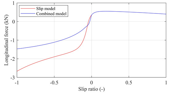
Figure 5.
Tire longitudinal force vs. slip ratio on clayey loam with a vertical load of 1.5 kN. The blue graph was produced by the combined tire model, which swaps between the skid and slip model, and the red graph was produced by the slip model.
For modeling the multipass effect, the approach developed by Senatore and Sandu was utilized [38]. As described by Holm, the changes in terrain properties following each pass are primarily a function of slip [88]. The more slip the tire has, the stronger its effect on the soil is. The multipass effect influences the density , cohesion , and shear deformation modulus utilizing the following equations:
where , , and are constants, is the slip ratio during the previous pass, and is the number of passes. The values for , , and were acquired from [38]. In addition to the parameter changes, the soil is also compacted by the tires. Thus, due to the robot front and rear axles having the same track width, the rear tires traverse in the ruts created by the front tires. Furthermore, some of the tines on the harrow traverse in the ruts left by the tires of the robot, which in turn affects the tine forces. In the developed simulation model, the ground was given a resolution of 1 cm. The values for soil density, cohesion, shear deformation modulus, and ground height used for calculating the tire forces of the rear tires are taken as the average of each of the points currently in contact with the tire.
3.3. Robot Equations of Motion and Harrow Dynamics
The dynamics of the robot is described by Equations (38)–(40). The longitudinal (x), lateral (y), and vertical (z) axes and coordinates referred to in the following sections refer to the world-fixed coordinate system. It should be noted that the points at which the resultant forces of the normal stress and tangential stress affect the tires are not the same. Hence, the longitudinal and vertical components of the normal and shear stress resultant forces are separated in Equation (40). In previous tire–soil interaction models, it has been common to make the assumption that all tire forces always apply at the bottom of the tire [38,39]. Aerodynamic drag was omitted from the model due to the low speeds at which the robot would operate. The longitudinal dynamics of the robot in the developed model is described as
where and represent the longitudinal force produced by the front and rear tires; is the longitudinal force, also known as draft force, exerted on the hook at the back of the robot by the harrow; and is the longitudinal acceleration of the center of gravity (CoG) of the robot. The vertical dynamics is described as
where and are the vertical forces produced by the front and rear tires, is the vertical force exerted on the hook by the harrow, and is the vertical acceleration of the CoG of the robot. The rotational dynamics of the robot with respect to the lateral axis is described as
where , , , , , , , and represent the longitudinal and vertical forces at the front and rear tires caused by the shear () and normal () stresses; , , , , , , , and are the longitudinal and vertical coordinates of the shear and normal stress resultant forces; and are the longitudinal and vertical coordinates of the CoG; and are the vertical speeds of the front and rear wheels; and and are the inertia and rotational acceleration of the robot.
Figure 6 shows a schematic of the forces affecting the robot and their application points. As can be deduced from Equations (24)–(27), the application points of the tangential () and normal ) tire forces can vary within the contact patch. The case shown in Figure 6 represents the AWD robot where both the front and rear axles provide tractive force. The height of the ground behind the tires represents the height of the ruts left by the tires.
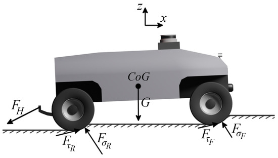
Figure 6.
Schematic of the forces affecting the robot.
The harrow model was designed based on the approach originally developed by Söhne [81]. In the model, the longitudinal and vertical tine forces depend on the tine dimensions, speed, depth, and angle in addition to the cohesion, density, and internal friction of the soil. The relevant geometry of the soil deformation used in the calculations is presented in Figure 7, where represents the shear angle of the soil and represents the angle of the tine.
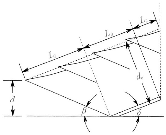
Figure 7.
Segment of soil being operated on by a tine (adapted from [89]).
The longitudinal and vertical forces ( and ) produced by a tine are calculated using the following Equations [89]:
where b and are the width and speed of the tine, and are the cohesion and acceleration forces the soil exerts on the tine, is the coefficient of friction between the tine and the soil, and Z is a support variable. For the harrow dynamics calculations, it is assumed that the forces and apply to the center point of the tine. The longitudinal dynamics of the harrow is described as
where represents the longitudinal force produced by a harrow tire, is the longitudinal force exerted on the harrow by the hook, and represent the total longitudinal force produced by the front and rear row of tines, is the mass of the harrow, and is the longitudinal acceleration of the CoG of the harrow. The value of is equal and opposite to . The vertical dynamics of the harrow is described as
where represents the vertical force produced by a harrow tire, is the vertical force exerted on the harrow by the hook, and represent the total vertical force produced by the front and back row of tines, and is the vertical acceleration of the CoG of the harrow. The value of is equal and opposite to . The rotational dynamics of the harrow is described as
where , , , and represent the longitudinal and vertical forces of a harrow tire caused by the shear () and normal () stresses; , , , and are the longitudinal and vertical coordinates of the shear and normal stress resultant forces; , , , and are the longitudinal and vertical coordinates of the tines in the front and back rows; and are the longitudinal and vertical coordinates of the CoG of the harrow; is the vertical speed of the harrow wheels; and and are the inertia and rotational acceleration of the harrow. Figure 8 shows a schematic of the forces affecting the harrow and their application points. The lighter ground color behind the tires represents the height of the ruts left by the harrow tires.
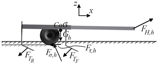
Figure 8.
Schematic of the forces affecting the harrow.
3.4. Simulation Parameters
The parameters of the robot are presented in Table 1. As was mentioned earlier, the robot was modeled to be the size of a typical ATV. The dimensions of the chassis and tires were made to match those of an ATV the Faculty of Agriculture and Forestry at the University of Helsinki is in possession of, the FBH version of the Blade ATV by Taiwan Golden Bee Co., Ltd. [90]. The mass of the chassis without the engine and drivetrain was measured to be approximately 286 kg. The height of the center of gravity was defined as 0.6 m. The weight distributions of the five different models are shown in Table 2.

Table 1.
Robot parameters.
Table 2.
Static weight distributions of the five models used in the simulations.
The efficiency map for a permanent magnet motor, shown in Figure 9, was acquired from the Autonomie software, which contains a vast library of powertrain components [91]. The map combines the efficiency of both the electric motor and the inverter. The map shown in the figure is for the AWD robot, which uses two motors powering each axle independently. For the RWD and FWD models, the motor torque was doubled so that the RWD, FWD, and AWD versions would all feature the same total maximum power and torque. The gear ratio of the final drive was selected such that the theoretical maximum speed of the robot would be 20 km/h. With the chosen gear ratio, the robot would operate at the region of maximum motor efficiency when driving at typical operation speeds of 5 to 10 km/h.
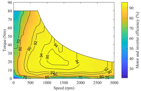
Figure 9.
Efficiency map of the electric motor and inverter for the AWD model. The map for the RWD and FWD models is identical but the torque values on the y axis are doubled.
For the battery pack, data for the dependence of the internal resistance and the open-circuit voltage on the SOC were acquired from a previous study examining nickel manganese cobalt (NMC) battery cells, more specifically NMC111 [92]. The battery pack was configured to operate at 48 V and have an energy capacity of approximately 17 kWh.
The harrow parameters are presented in Table 3. The harrow was modeled as a typical compact tine harrow with a total of ten tines. The back row of tines is mounted at the back of the harrow and the front row is mounted 0.8 m ahead of the back row. The tires are mounted 0.5 m in front of the back end of the harrow.
Table 3.
Harrow parameters.
The parameters for the two soils used in the simulations are presented in Table 4. The parameters were acquired from previous works by Wong as well as Senatore and Sandu [38,93]. The parameters for slip sinkage and multipass calculations, shown in Table 5, were acquired from the aforementioned research by Senatore and Sandu [38].
Table 4.
Parameters for the sandy loam and clayey loam soil types used in the simulations.
Table 5.
Tire parameters for slip sinkage and multipass calculations.
3.5. Control
The control system of the robot model utilizes a proportional speed controller. The aim with the choice of controller type was to facilitate a fair comparison between the different models. Thus, a simple proportional controller was chosen. As is described later, a traction control (TC) system was also added to ensure that none of the models would be disadvantaged by excess wheelspin causing significant energy losses. The proportional controller outputs a value from −1 to 1. The control value is then multiplied by the maximum torque of the motor at the current rotational speed to acquire the torque command for the electric motor based on the difference between the reference speed and the actual speed of the robot. During deceleration maneuvers, the torque demand may be negative, in which case the motor slows the robot down with regenerative braking. As has been discussed in previous works, there is a distinct lack of well-established reference operation cycles for wheeled agricultural machines [94,95]. Thus, a basic reference operation cycle was defined for the simulations to facilitate a fair comparison between the different robot models. The reference cycle describes the target speed of the robot as a function of distance traveled. Before the actual cycle begins, there is first a precycle portion where the robot moves for three meters. The robot initially spawns and sinks into the ground, and thus there are no ruts yet formed by the wheels. The purpose of the precycle maneuver was to ensure that the rear wheels of the robot would be in the ruts left by the front wheels when the actual cycle begins. The reference cycle starts with an acceleration maneuver at 0.1 g, which continues until the cycle reaches the defined maximum speed. After the robot has traversed 100 m on the operation cycle, a deceleration maneuver at 0.15 g is then carried out until the robot has stopped.
Three different tine depths were simulated with each of the five models on both of the soils: 5, 10, and 15 cm. The tine vertical positions were defined such that the actual average tine depths during the simulations would be approximately at the target depth when the harrow tires would sink into the soil, thus lowering the tines from their initial depth. In the context of this research, the term “operation cycle” is considered to encompass both the speed of the robot as well as the tine configuration.
Four different target speeds were defined: 4, 6, 8, and 10 km/h. Thus, simulation results from a total of 120 different combinations of five robot models, two soil types, three tine depths, and four target speeds were acquired. Examples of the operation cycles are shown in Figure 10, which shows cycles completed by the AWD model with four different target speeds on clayey loam. For each combination of robot model, soil type, tine depth, and target speed, the gain value of the proportional controller was iterated on to ensure the robot would provide sufficient torque to the wheels to reach the target speed. However, with some combinations, the robot was unable to reach the target speed even with full throttle applied, as is shown in the Results and Discussion Section.
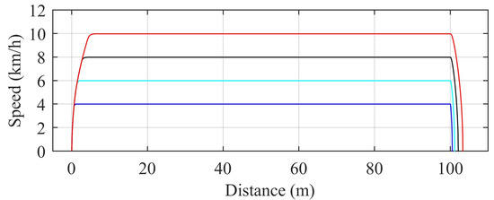
Figure 10.
Operation cycles with the simulated AWD robot on clayey loam with varying target speeds (4 km/h (blue), 6 km/h (cyan), 8 km/h (black), 10 km/h (red)) and a tine depth of 10 cm.
The control system features a simple TC algorithm that prevents the driven wheels from slipping excessively. The TC starts to limit the torque demand provided by the controller when the slip ratio of the driven wheels gets near the ratio at which maximum longitudinal tire force is achieved. The behavior of the longitudinal tire force as a function of slip is heavily dependent on the soil properties. Thus, the threshold values at which the TC would start to intervene were defined separately for each soil type. Utilizing the tire–soil model described in Section 3.2, the threshold values were determined for each soil and model combination by observing the optimal slip with an approximated 10% vertical load transfer to the rear axle. The determination of the threshold values revealed the optimal slip to vary significantly between sandy loam and clayey loam. On sandy loam, the optimal slip ratio was found to be between 0.25 and 0.35 depending on the robot model, while on clayey loam, the range was from 0.10 to 0.18.
In addition, an algorithm controlling the distribution of motor power between front and rear axles was devised for the AWD robot. At lower torque levels, the algorithm provides more power for the rear axle than the front axle to make use of the greater traction available at the rear. As the control value output by the proportional controller increases, the power difference between the axles reduces. At maximum throttle (control value of 1), both motors provide maximum torque. This type of power distribution control was found to reduce the energy consumption of the AWD robot. The power distribution is performed with the following equations:
where and are the new weighted control signals for the rear and front axles, is the original control value output by the proportional controller, and is the power distribution factor. With the weighted control values for the axles formulated in this way, the average of the rear and front control values is still equal to the original control value. As can be seen in the equations, a higher power distribution factor will shift the power distribution further to the rear axle. By iterating through different power distribution factors in varying conditions, it was determined that a factor of 1.4 would provide the overall lowest energy consumption.
4. Results and Discussion
The robot–harrow model was simulated with a fixed time step of 1 ms. The simulations had on average a real-time factor of 0.163 (i.e., simulating 1 s of robot operation took approximately 6.14 s). The simulations were conducted using an AMD Ryzen 9 5900X processor running at an average clock speed of 4.6 GHz.
In this section, the simulation results are presented and discussed. In Section 4.1, success matrices are presented for all of the models in all operation cycles and soils. The matrices describe whether the model was able to complete the cycle and what the energy consumption per unit distance was. The energy consumption distributions are also presented as box plots. In the subsequent subsections, the different models are compared by examining example cases. In Section 4.2, the performances of the models with a light workload are compared, with particular focus on the FWD configuration. Section 4.3 compares the performances of RWD and AWD, and the final subsection examines the effect the operation cycles had on the energy consumption and considers the limitations of the conducted research.
4.1. Success Matrices and Energy Consumption Variation
The success matrices for each model on both soil types are presented in Figure 11. In the figure, each matrix cell contains the energy consumption per unit distance (Wh/km) achieved by the model on the operation cycle. In cases where the model was unable to achieve the target speed, the matrix cell is colored black.

Figure 11.
Success matrices for each model. The matrices describe whether the model was able to achieve the target speed with the given tine depth. The numbers in the cells describe the energy consumption (Wh/km).
Figure 11 shows that on the sandy loam soil, both RWD models and the AWD model were able to complete all combinations of target speed and tine depth. On the other hand, the FWD1 model was unable to reach the target speed with any tine depth deeper than 5 cm, while the FWD2 model could not reach the target speed with a tine depth of 15 cm. On the clayey loam soil, the FWD1 model was unable to move at all, and the FWD2 model could only reach the target speed with the shallowest tine depth setting. The RWD1 model was unable to reach target speeds of 8 and 10 km/h with a tine depth of 15 cm, while the RWD2 and AWD models were still able to successfully complete all of the cycles on clayey loam.
The success matrices show that, as expected, the highest energy consumption occurred in the operation cycle with the highest target speed and tine depth. However, it can also be noticed in the figure that the lowest energy consumption did not occur in the combination of lowest speed and tine depth. Instead, the lowest energy consumption was achieved by each model with a tine depth of 5 cm and a target speed of either 6 or 8 km/h instead of the lowest speed of 4 km/h. This is primarily a consequence of the auxiliary device power demand. As the auxiliary power demand is constant, completing the cycle faster reduces the total energy used by the auxiliary devices. These results demonstrate the importance of finding the optimal speed for achieving the lowest energy consumption and thus maximizing the operating range. Figure 12 shows the energy consumption distributions for the models that were able to complete all of the cycles.
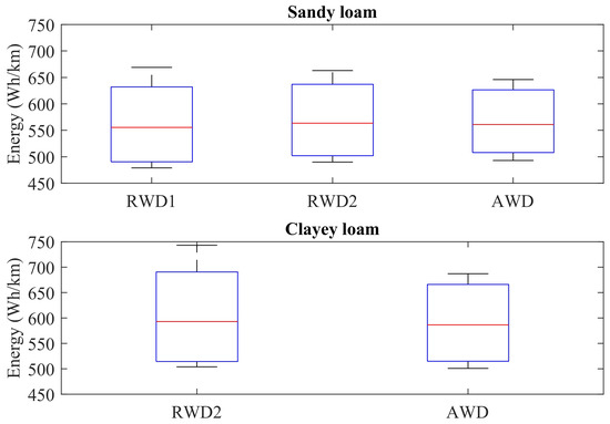
Figure 12.
Energy consumption distributions for both soils presented as box plots. Only models that were capable of executing all tine/speed combinations are included.
It is also worth noting that although the robot was capable of regenerative braking, on most operation cycles there was no regeneration due to the high resistive forces slowing the vehicle down without the need for braking. Only on sandy loam with a tine depth of 5 cm was any regenerative braking performed. Even then, the highest amount of energy regenerated was only 0.035 Wh by the AWD model in the cycle with a 10 km/h target speed. Although more energy could potentially be regenerated with a harder braking maneuver, the results indicate that regenerative braking provides negligible energy-efficiency benefits during field operations.
Some comparisons of the influence of the different factors can be drawn based on the results shown in Figure 11. On sandy loam, increasing the tine depth from 5 to 10 cm increased the energy consumption by 15.2% on average. The increase from 5 to 15 cm caused the consumption to rise by 29.7%. For clayey loam, the respective values were 16.7% and 36.5%. This result shows that the tine depth had more influence on clayey loam. Increasing the target speed from 4 km/h to 6, 8, and 10 km/h caused an average consumption change of −1.9%, −1.4%, and 1.0% on sandy loam. On clayey loam, the respective percentages were −1.8%, −1.5%, and 0.9%. However, it should also be noted that the influence of the target speed was highly dependent on the tine depth. For instance, with the RWD1 model on sandy loam, consumption reduced by 3.2% when increasing the speed from 4 km/h to 10 km/h with a tine depth of 5 cm. When the tine depth was 15 cm, the same increase in speed increased the consumption by 5.4%. Nevertheless, the results make it clear that the implement configuration has significantly more influence on the energy consumption compared to the robot speed. Overall, energy consumption on clayey loam was on average 6.1% higher than on sandy loam.
Energy consumption per unit area values can also be derived based on the results, given the 1.3 m width of the harrow. For example, on the clayey loam soil, the consumption of the AWD model would vary from 3.85 to 5.28 kWh/ha. With the 17.3 kWh battery capacity, the area the robot would be able to cover with a single charge would be between 3.27 and 4.49 ha. For the RWD2 model, that variation would be from 3.03 to 4.46 ha. On the sandy loam soil, the range of the AWD robot would vary between 3.48 and 4.56 ha. The highest range (4.70 ha) would be achieved by the RWD1 version with a target speed of 8 km/h and tine depth of 5 cm on sandy loam. Overall, these results demonstrate the significant effect soil properties, implement configuration, and the powertrain layout of the robot have on the energy consumption and operating range. Furthermore, the relatively limited area the robots can cover on a single charge underlines the importance of utilizing fleets of such machines to ensure high working rates. Due to the novelty of electric agricultural machinery, direct comparisons to these energy consumption results cannot be found in the existing literature. In a simulation study comparing different powertrains for an agricultural tractor, Lajunen found the energy consumption of an 8.6-ton electric tractor in tillage operations to range from approximately 33 to 49 kWh/ha depending on the workload [96]. Thus, the results presented here show that an ATV-sized electric agricultural robot has approximately one-tenth the energy consumption of a full-scale electric agricultural tractor.
As can be observed in Figure 12, the AWD model had the lowest consumption variation on both soil types. In other words, the results demonstrate that AWD can provide the highest robustness against energy consumption variations. However, the RWD1 model had a lower average consumption on sandy loam compared to the AWD model (562 vs. 566 Wh/km), showing the lighter weight achieved with a single driven axle can prove advantageous with lighter workloads on certain soils. It is interesting to note that the RWD2 model also had lower variation in the energy consumption compared to the RWD1 model on sandy loam despite having a higher average consumption. The results between the two RWD models indicate the importance of configuring electric agricultural robots optimally for the given workload requirements and the soil they will operate on. On the clayey loam soil, the AWD model had a lower average consumption (590 vs. 604 Wh/km) as well as lower minimum (501 vs. 504 Wh/km) and maximum (687 vs. 743 Wh/km) consumptions compared to the RWD2 model. The results make it clear that the superior tractive performance gives the AWD configuration a significant advantage on soils that are difficult to traverse.
4.2. Performance Comparison with a Light Workload
Figure 13 shows a breakdown of the energy losses on sandy loam with a tine depth of 5 cm and target speed of 4 km/h, which all five models were able to complete. It can be seen in the figure that the primary reason for the RWD1 model achieving the lowest consumption in this particular operation cycle was that it had the lowest tire losses. The tire losses include the losses due both to slip and to rolling resistance. The tire losses of the RWD1 model were 5.4% lower compared to the AWD model. For all models, robot tire losses were the largest source of energy losses. The tire losses accounted for 57.0, 57.7, 60.6, 58.3, and 58.2% of the total losses for the RWD1, RWD2, FWD1, FWD2, and AWD models, respectively. These percentages are higher than what Lajunen et al. found when they simulated a 10-ton electric tractor in tillage operations [9]. Their results showed the tire losses to range from 40 to 45% of the total losses with light workloads. However, the simulation model they used calculated tire losses with a simple rolling-resistance-based model without consideration for slip or tire sinkage.

Figure 13.
Distribution of energy losses on sandy loam with a tine depth of 5 cm and a target speed of 4 km/h.
Interestingly, even the FWD2 model had lower tire losses and overall consumption compared to the AWD model, which again showcases how the heavy weight of the AWD system can prove a noticeable disadvantage with light workloads. However, the high energy use of the FWD1 model shows the importance of having sufficient vertical load on the driven axle, as the tire losses were 13.5% higher compared to the FWD2 model. The performance of the FWD1 model is further examined in Figure 14, Figure 15 and Figure 16.
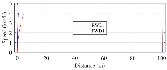
Figure 14.
Comparison of the robot speed between the RWD1 and FWD1 models on sandy loam with a tine depth of 5 cm and a target speed of 4 km/h.
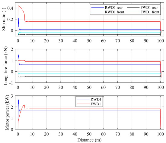
Figure 15.
Comparison of slip ratios, longitudinal tire forces on each axle, and electric motor power for the RWD1 and FWD1 models on sandy loam with a tine depth of 5 cm and a target speed of 4 km/h.
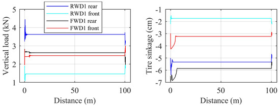
Figure 16.
Vertical loads on the axles and tire sinkages for the RWD1 and FWD1 models on sandy loam with a tine depth of 5 cm and a target speed of 4 km/h.
Figure 14 shows that the FWD1 model was slower to accelerate compared to the RWD1 model. It took the FWD1 model 3.2 s longer to complete the cycle. One consequence of a slower cycle is that the energy consumption of the auxiliary devices is higher. In this operation cycle, the auxiliary consumption for the FWD1 model was 3.2% higher for the FWD1 model compared to the RWD1 model. The causes for the poor acceleration of the FWD1 model can be seen in Figure 15 and Figure 16. It should be noted that the longitudinal tire force graphs represent the combined forces of the tires on a given axle.
As Figure 15 shows, the FWD1 model had significantly higher slip on the driven axle compared to the RWD1 model. The lower vertical load on the driven axle the FWD1 model had, which can be seen in Figure 16, limited the traction. In addition, the higher vertical load on the nondriven axle with the FWD1 model caused the tires on the axle to produce more negative longitudinal force, which in turn necessitated the driven axle to produce higher positive longitudinal force. As can be seen in Figure 15, during the constant speed portion of the cycle, the front tires of the FWD1 model generated approximately 40% higher longitudinal force than the rear tires of the RWD1 model. During the constant speed operation, the output power of the motor was 11.4% higher for the FWD1 model. Another issue with the FWD1 model is visible in Figure 16; the high slip of the front tires caused them to sink deeper into the soil. Consequently, the rear tires of the FWD1 model also sank deeper due to the ruts left by the front tires being deeper. It is interesting to note that the motor power difference was clearly smaller between the two models than the difference in the longitudinal force of the driven wheels. In fact, during the constant speed portion of the cycle, the FWD1 model had lower motor torque than the RWD1 model. In other words, the FWD model had higher tractive efficiency at the driven axle. This is due to the RWD1 model’s driven wheels sinking deeper into the soil, causing significantly increased rolling resistance. Yet, the RWD model was able to be more energy-efficient overall due to the high resistance caused by the rear tires of the FWD version causing high slip of the front tires.
4.3. Comparison of RWD and AWD
Figure 17 and Figure 18 present a comparison of the RWD1, RWD2, and AWD models in the most energy-intensive cycle on the sandy loam soil.
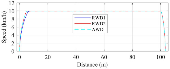
Figure 17.
Comparison of the robot speed between the RWD1, RWD2, and AWD models on sandy loam with a tine depth of 15 cm and a target speed of 10 km/h.

Figure 18.
Distribution of energy losses on sandy loam with a tine depth of 15 cm and a target speed of 10 km/h.
The results presented in Figure 17 and Figure 18 show that the differences in the performance of the three models in the examined operation cycle were minor. The RWD2 and AWD models were able to accelerate at approximately the same rate, while the RWD1 model was slightly slower to reach the target speed. As Figure 18 shows, the tire losses were the primary cause of the differences in energy consumption. The tire losses were 340.6, 334.8, and 320.2 Wh/km for the RWD1, RWD2, and AWD models. In the constant speed section of the cycle, the RWD1 version had the highest slip ratio (0.069) on the driven axle, while the RWD2 model had a slip ratio of 0.035. For the AWD model, the front tires had a slip ratio of 0.049 and the rear tires 0.010. The RWD1 model has slightly less traction available at the driven axle due to the more frontward weight distribution compared to the RWD2 model. The more frontward weight distribution also caused the front tires to produce more resistance due to sinking deeper into the soil. In the case of the operation cycle examined in Figure 17 and Figure 18, during the constant speed section, the front tires of the RWD1 model produced a longitudinal force of −176 N, while the value for the RWD2 model was −90 N.
Although the differences in energy consumption between the RWD and AWD models were minor on the sandy loam soil, significantly higher performance variation could be observed on the clayey loam soil, where the RWD1 model was not able to complete the most energy-intensive operation cycles. The RWD2 and AWD models are compared in Figure 19, Figure 20 and Figure 21 in the operation cycle with a tine depth of 15 cm and target speed of 10 km/h.
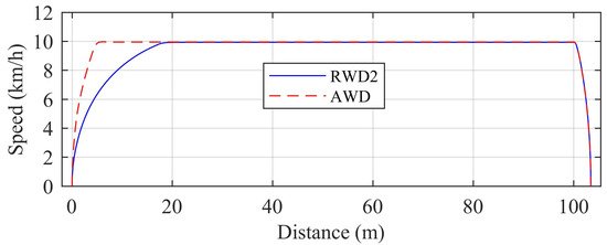
Figure 19.
Comparison of the robot speed between the RWD2 and AWD models on clayey loam with a tine depth of 15 cm and a target speed of 10 km/h.

Figure 20.
Distribution of energy losses on clayey loam with a tine depth of 15 cm and a target speed of 10 km/h.
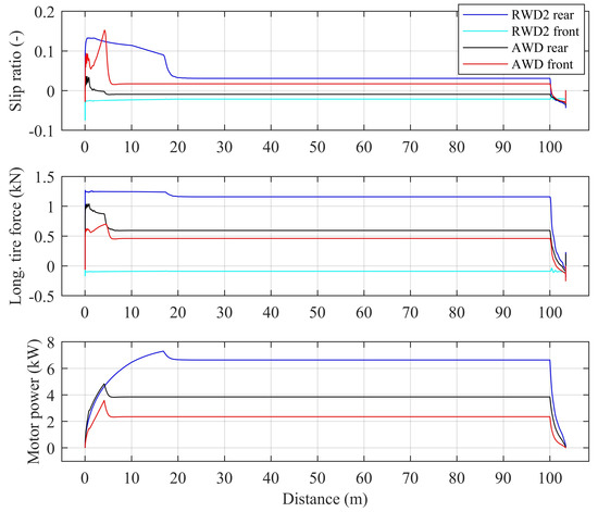
Figure 21.
Comparison of slip ratios, longitudinal tire forces on each axle, and electric motor power for the RWD2 and AWD models on clayey loam with a tine depth of 15 cm and a target speed of 10 km/h.
Despite the similar performance between the RWD2 and AWD models on the sandy loam soil, Figure 19 shows that in the most challenging operation cycle on the clayey loam soil, the AWD version of the robot was able to accelerate faster due to higher traction. It took the AWD model approximately 3.5 s to reach the target speed of 10 km/h, while for the RWD2 version it took 11.0 s. The energy loss distributions for both models are shown in Figure 20, where it can be seen that the tire losses were significantly higher for the RWD2 model. The 3.7 s longer cycle of the RWD2 model also caused the auxiliary device losses to be almost 6% higher. The overall energy consumption was 7.53% lower for the AWD robot. The tractive performance of the models is further examined in Figure 21.
In Figure 21, the motor power graph shows that during the constant speed section, the motor output power of the RWD2 robot was 6.63 kW, while the combined output of the two motors of the AWD model equated to 6.20 kW. During acceleration, the peak motor power of the RWD2 model was 7.3 kW, while the AWD version reached a combined motor power of 8.4 kW. The lower peak power of the RWD2 robot during acceleration was due to the traction control limiting motor power to prevent excessive slip. Additionally, the motor power plots for the AWD model demonstrate the effect of the motor power distribution system described in Section 3.5, as the rear motor produced a higher power output compared to the front motor. Yet, the front tires still had higher slip, potentially indicating that further consumption reductions could be achieved with more accurate slip control. Overall, the results on clayey loam demonstrate the substantial energy consumption reductions that can be achieved with an AWD system in challenging conditions due to the better tractive performance.
4.4. Effect of Operation Cycle on Energy Consumption
To further examine the energy consumption impact of the workload, Figure 22 presents energy loss distributions for the RWD2 on the clayey loam soil in four different operation cycles. The energy loss distributions show that the largest increases in energy consumption were caused by the losses due to tine forces. Comparing the cycle with a 5 cm tine depth and 6 km/h target speed to the cycle with a 15 cm tine depth and 10 km/h target speed, the tine losses increased by 307%. Furthermore, the harrow tire losses increased by 25% due to the tires sinking deeper with the increased tine depth. Comparing the two cycles with a tine depth of 5 cm shown in Figure 22, the tine losses increased by 21%. On the other hand, increasing the tine depth from 5 cm to 15 cm with a 6 km/h speed increased the tine losses by 245%. Thus, the tine forces and consequently the draft force are influenced significantly more by the tine depth than the driving speed.
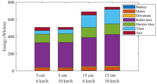
Figure 22.
Distribution of energy losses with the RWD2 model on clayey loam with different speeds and tine depths.
The robot tire losses also increased due to the higher resistance and the increased target speed necessitating higher tractive force and thus higher slip. Additionally, the higher tine forces caused by increased tine depth resulted in the rear tires sinking deeper into the soil, further reducing the tractive efficiency of the tires. Comparing the lightest and most energy-intensive cycles shown in Figure 22 shows that the robot tire losses increased by 27.3%. The robot tire losses increased from 49.5 to 56.9% as a proportion of the total energy consumption. This result is in contrast to the results found by Lajunen et al. with a simulated 10-ton electric tractor, which showed the tire losses as a proportion of the total energy consumption to decrease from 45 to 21% going from a light workload to a heavy workload [9]. However, as their research did not utilize a tire–soil interaction model and simulated tire losses with a rolling-resistance model, the workload had minimal effect on the tire losses. The contrast between the findings shows how important it is to utilize detailed tire–soil interaction models to properly include the dependence of tire losses on the workload.
It can also be observed in Figure 22 that the energy intensity of the operation cycle significantly affected the battery losses. In the lightest cycle, the battery losses were only 1.3 Wh/km. With a tine depth of 15 cm and target speed of 10 km/h, the battery losses increased to 6.3 Wh/km. Yet, even in the most challenging cycle, the battery losses still only accounted for 0.85% of the total losses. The drivetrain losses also increased as a function of the power throughput, with the most energy-intensive cycle having 54% higher drivetrain losses compared to the lightest cycle. The motor losses also increased by 26%.
Figure 23, Figure 24, Figure 25 and Figure 26 present results related to the harrow model. In the figures, the results of the RWD2 model on the clayey loam soil are compared in four operation cycles. In Figure 23, the draft force exerted by the harrow on the hook of the robot during the constant speed section varies from 508 to 1069 N. It can also be seen that the tine depth affected the draft force more than the driving speed. However, it can also be observed that the effect of the speed increased with the tine depth. When increasing the speed from 6 to 10 km/h with a tine depth of 5 cm, the draft force increased by 7.7%. On the other hand, increasing the speed from 6 to 10 km/h with a tine depth of 15 cm caused a draft force increase of 13%. A similar effect can be seen with the vertical force as well.
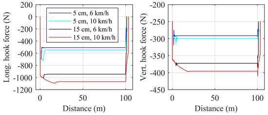
Figure 23.
Longitudinal (draft) force and vertical force affecting the hook of the RWD2 model on clayey loam soil with different speeds and tine depths.

Figure 24.
Total longitudinal and vertical tine forces on clayey loam soil with different speeds and tine depths.
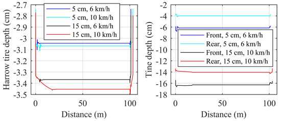
Figure 25.
The depths of the harrow tires and the tips of the front and rear rows of tines on clayey loam soil with different speeds and tine depths.
Figure 26.
Slip ratio and the longitudinal force of the harrow tires on clayey loam soil with different speeds and tine depths. The longitudinal force is the combined force of both harrow tires.
The higher resistance on the hook with heavier workloads goes to further explain the increase in robot tire losses between the operation cycles seen in Figure 22. Similarly, the more negative (downward) vertical force on the hook also contributed to the increased tire losses due to forcing the tires to sink deeper into the soil. The tine forces in the operation cycles are shown in Figure 24.
The tine force results in Figure 24 show the significant influence the tine depth as well as the speed of the robot have on the tine forces. In the constant speed section, the longitudinal force ranged from 149 to 620 N and the vertical force from 129 to 532 N. The higher downward force also caused the harrow tires to sink deeper into the soil, as can be seen in Figure 25. Similar to Figure 23, the tine force results also show that the effect of the driving speed on the forces was more significant with a higher tine depth.
The slip ratio and the longitudinal force of the harrow tires are shown in Figure 26. Figure 25 shows that the harrow tires sank approximately 4.1 mm deeper in the most challenging cycle compared to the lightest cycle. The resulting increased slip and longitudinal force can be seen in Figure 26. Thus, the results demonstrate how the increased tine depth and robot speed not only increase the resistance caused by the tines but also further increase the resistance caused by the harrow tires as well. Additionally, the depths of the front and rear tine rows are presented in Figure 25 for two of the operation cycles. On both operation cycles, the front row sank deeper than the rear row, while the average depth remained close to the target value. The front row sinking deeper was caused by the harrow pitching forward due to the rear tires of the robot sinking deeper into the soil than the harrow tires. For example, in the cycle with a tine depth of 15 cm and target speed of 10 km/h, the rear tires of the robot sank to a depth of 5.31 cm, while the harrow tires sank to a depth of 3.45 cm. The high influence of the tine depth on the energy consumption seen in the results underlines the importance of optimizing the configuration of the implement pulled by an electric agricultural robot.
Certain simplifications in the simulation approach limited the scope of the results. Firstly, the speed profiles of the reference operation cycles were simplistic, with linear accelerations and decelerations, and they were not optimized for the different models and soils separately. In addition, the robot was assumed to operate on flat ground with no uphills or downhills. The robot was also not modeled to feature any suspension, and the tires were assumed to be rigid. The assumption of tire rigidity was considered to be acceptable in the context of a compact robot with a small tire size. For larger machines, the flexibility of the tires would have to be included in the model due to larger tires deforming significantly more. Furthermore, only the longitudinal dynamics of the robot were modeled. In real-world operations, the robot would have to carry out cornering maneuvers, which would affect the energy consumption. The simulations also only considered one type of agricultural implement. Small wheeled electric robots can be utilized to perform various types of operations on agricultural fields. However, the utilization of a tine harrow in this article was considered to be valuable due to the proven and well-known modeling technique originally established by Söhne and the ability to significantly affect the draft force by changing the tine configuration. With the presented simulation approach, it would be easy to modify the implement model to represent other types of farm implements in future studies.
Furthermore, the auxiliary device power was approximated as being constant. At high battery power, the cooling power demand would likely increase. Another limitation of the study was the limited number of weight distributions tested for the different models. Further iteration could be conducted to find the optimal weight distributions for RWD, FWD, and AWD. In particular, the viability of an FWD powertrain configuration appears to be highly impacted by the weight distribution. As was indicated by the results, making FWD viable in an electric agricultural robot would require an unusually frontward weight bias. Achieving an even more frontward weight bias than what was used would require consideration for the viability of novel design ideas, which was seen as out of the scope of this research. In addition, another further iteration process could be conducted for varying the tire sizes as well to optimize the contact pressure and tire sinkage. Furthermore, for the AWD model, it might be advantageous to utilize motors with different power ratings on the front and rear axles rather than trying to optimize the power distribution between the front and rear axles with control logic as was performed in this study. However, more detailed optimization of the robot dimensions, powertrain configuration, and control were considered out of the scope of this study.
5. Conclusions
In this paper, a novel simulation model of an electric agricultural robot pulling a tine harrow was presented. The model features an electric powertrain model, a tire–soil interaction model with deformable terrain, and a harrow dynamics model. Versions of the robot with different powertrain configurations (FWD, RWD, and AWD) were created. For the single-axle-driven models, two different weight distributions were tested. Simulations were conducted on two soil types: sandy loam and clayey loam. The models were simulated on various operation cycles where the target speed and tine depth were varied.
The results demonstrated that the optimal powertrain configuration is highly dependent on the workload and type of soil the robot operates on. With lighter workloads, the RWD models were found to be capable of lower energy consumption compared to the AWD model, with the highest difference being 3.5%; while AWD has superior traction compared to single-axle-driven configurations, it is disadvantaged by the higher mass. In the most energy-intensive cycles, the AWD model outperformed the RWD versions. The advantage was higher on the clayey loam soil, where AWD outperformed RWD by 7.5% in the most challenging operation cycle. Interestingly, one of the FWD models was also capable of lower energy consumption than the AWD version in the lightest operation cycles on sandy loam. However, the FWD models were not capable of completing all of the operation cycles on either soil type due to the lack of traction, with the performance being particularly poor on clayey loam. The FWD model with a higher frontward weight distribution (70%) performed significantly better than the version with a 60/40 weight distribution. The weight distribution was also found to have a clear impact on the performance of the RWD configuration. With light workloads, the version with a more even weight distribution (40/60) had lower energy consumption. However, the higher the workload, the more the advantage shifted to the model with a more rearward weight distribution (30/70).
Another aspect the results clearly showed was that the speed electric agricultural robots operate at must be carefully considered. Due to the auxiliary device losses, the lowest energy consumption for a given distance or area that needs to be covered is not necessarily achieved by driving at the slowest feasible speed. The speed choice must be balanced between this fact and the increasing resistance of the implement and tractive force requirement of higher speeds. The results demonstrated the high energy-consumption variations that can be caused by different harrow configurations and robot speeds. With the tines at the highest depth and a robot target speed of 10 km/h, the draft force increased by 113% compared to the shallowest tine depth and target speed of 4 km/h. The indirect losses caused by the harrow also increase with the workload due to the losses of the robot tires increasing due to higher sinkage and greater traction demands leading to higher slip.
To facilitate the widespread implementation of autonomous electric agricultural robots, future work based on the research presented here should focus on optimization of the robot design as well as fleet management. The modeling approach presented can be used to optimize design aspects such as tire size and width, wheelbase, and longitudinal weight distribution. The model could also be used to investigate control optimization to further enhance the tractive efficiency. Models for other implements could be added as well, for example, by utilizing the implement force equations of ASAE. In addition, the model could be extended to be three-dimensional so that the energy losses caused by cornering maneuvers could be simulated as well. The modeling approach can serve as a useful tool for developing strategies for managing fleets of agricultural robots. Ensuring high working rates on fields by autonomous electric robots is a challenging task that requires high-fidelity simulation tools to optimize the design of the robots, the amount of robots used, and the energy management strategies used for controlling and charging the robots.
Author Contributions
Conceptualization, K.K. and A.L.; data curation, K.K. and A.L.; formal analysis, K.K.; funding acquisition, A.L.; investigation, K.K.; methodology, K.K. and A.L.; project administration, A.L.; resources, K.K. and A.L.; software, K.K.; supervision, A.L.; visualization, K.K.; writing—original draft preparation, K.K.; writing—review and editing, K.K. and A.L. All authors have read and agreed to the published version of the manuscript.
Funding
The authors would like to acknowledge the financial support from the AgroSim project (2022–2025), which is funded by the Henry Ford Foundation of Finland.
Data Availability Statement
The developed simulation model is available at the following open-source repository, created by the authors: https://github.com/Kivakis/eAgriBot (created on 17 January 2024). The result data may be provided by the authors upon request.
Acknowledgments
Open access funding provided by University of Helsinki.
Conflicts of Interest
The authors declare no conflicts of interest.
Abbreviations
The following abbreviations are used in this manuscript:
| ATV | All-terrain vehicle |
| AWD | All-wheel drive |
| CoG | Center of gravity |
| DEM | Discrete element method |
| FEM | Finite element method |
| FWD | Front-wheel drive |
| GHG | Greenhouse gas |
| ICE | Internal combustion engine |
| NMC | Nickel manganese cobalt |
| PV | Photovoltaic |
| RWD | Rear-wheel drive |
| SOC | State of charge |
| SOD | State of discharge |
| SPH | Smoothed particle hydrodynamics |
| TC | Traction control |
References
- United Nations, Department of Economic and Social Affairs, Population Division. World Population Prospects 2022. Available online: https://population.un.org/wpp/Graphs/DemographicProfiles/Line/900 (accessed on 1 January 2024).
- Ghobadpour, A.; Monsalve, G.; Cardenas, A.; Mousazadeh, H. Off-Road Electric Vehicles and Autonomous Robots in Agricultural Sector: Trends, Challenges, and Opportunities. Vehicles 2022, 4, 843–864. [Google Scholar] [CrossRef]
- Tubiello, F.; Salvatore, M.; Ferrara, A.; House, J.; Federici, S.; Rossi, S.; Biancalani, R.; Condor Golec, R.; Jacobs, H.; Flammini, A.; et al. The Contribution of Agriculture, Forestry and other Land Use activities to Global Warming, 1990–2012. Glob. Chang. Biol. 2015, 21, 2655–2660. [Google Scholar] [CrossRef] [PubMed]
- Climate Change and Agriculture in the EU. Available online: https://agriculture.ec.europa.eu/sustainability/environmental-sustainability/climate-change_en (accessed on 10 November 2023).
- Gerber, P.J.; Steinfeld, H.; Henderson, B.; Mottet, A.; Opio, C.; Dijkman, J.; Falcucci, A.; Tempio, G. Tackling Climate Change through Livestock: A Global Assessment of Emissions and Mitigation Opportunities; Food and Agriculture Organization of the United Nations (FAO): Rome, Italy, 2013. [Google Scholar]
- Lovarelli, D.; Bacenetti, J. Exhaust gases emissions from agricultural tractors: State of the art and future perspectives for machinery operator. Biosyst. Eng. 2019, 186, 204–213. [Google Scholar] [CrossRef]
- Ragazou, K.; Garefalakis, A.; Zafeiriou, E.; Passas, I. Agriculture 5.0: A New Strategic Management Mode for a Cut Cost and an Energy Efficient Agriculture Sector. Energies 2022, 15, 3113. [Google Scholar] [CrossRef]
- Hernandez-Escobedo, Q.; Muñoz-Rodríguez, D.; Vargas-Casillas, A.; Juárez Lopez, J.M.; Aparicio-Martínez, P.; Martínez-Jiménez, M.P.; Perea-Moreno, A.J. Renewable Energies in the Agricultural Sector: A Perspective Analysis of the Last Three Years. Energies 2022, 16, 345. [Google Scholar] [CrossRef]
- Lajunen, A.; Kivekäs, K.; Freyermuth, V.; Vijayagopal, R.; Kim, N. Simulation of Alternative Powertrains in Agricultural Tractors. In Proceedings of the 36th International Electric Vehicle Symposium and Exhibition (EVS36), Sacramento, CA, USA, 11–14 June 2023. [Google Scholar]
- Lagnelöv, O.; Larsson, G.; Nilsson, D.; Larsolle, A.; Hansson, P.A. Performance comparison of charging systems for autonomous electric field tractors using dynamic simulation. Biosyst. Eng. 2020, 194, 121–137. [Google Scholar] [CrossRef]
- Malik, A.; Kohli, S. Electric tractors: Survey of challenges and opportunities in India. Mater. Today Proc. 2020, 28, 2318–2324. [Google Scholar] [CrossRef]
- Engström, J.; Lagnelöv, O. An Autonomous Electric Powered Tractor—Simulation of All Operations on a Swedish Dairy Farm. J. Agric. Sci. Technol. 2018, 8, 182–187. [Google Scholar] [CrossRef]
- Lagnelöv, O.; Dhillon, S.; Larsson, G.; Nilsson, D.; Larsolle, A.; Hansson, P.A. Cost analysis of autonomous battery electric field tractors in agriculture. Biosyst. Eng. 2021, 204, 358–376. [Google Scholar] [CrossRef]
- Lagnelöv, O.; Larsson, G.; Larsolle, A.; Hansson, P.A. Life cycle assessment of autonomous electric field tractors in Swedish agriculture. Sustainability 2021, 13, 11285. [Google Scholar] [CrossRef]
- Olkkonen, V.; Lind, A.; Rosenberg, E.; Kvalbein, L. Electrification of the agricultural sector in Norway in an effort to phase out fossil fuel consumption. Energy 2023, 276, 127543. [Google Scholar] [CrossRef]
- Farokhi Soofi, A.; Manshadi, S.D.; Saucedo, A. Farm electrification: A road-map to decarbonize the agriculture sector. Electr. J. 2022, 35, 107076. [Google Scholar] [CrossRef]
- Beltrami, D.; Iora, P.; Tribioli, L.; Uberti, S. Electrification of Compact Off-Highway Vehicles—Overview of the Current State of the Art and Trends. Energies 2021, 14, 5565. [Google Scholar] [CrossRef]
- Thakur, A.; Venu, S.; Gurusamy, M. An extensive review on agricultural robots with a focus on their perception systems. Comput. Electron. Agric. 2023, 212, 108146. [Google Scholar] [CrossRef]
- Schneider, A.; Klabunde, F.; Buck, L.; Ohlhoff, M.; Reis, L.; Olvermann, M.; Kauffeld, S.; Engel, B.; Glatzel, G.; Schröder, B.; et al. Drawing transformation pathways for making use of joint effects of food and energy production with biodiversity agriphotovoltaics and electrified agricultural machinery. J. Environ. Manag. 2023, 335, 153811–153823. [Google Scholar] [CrossRef] [PubMed]
- Gorjian, S.; Ebadi, H.; Trommsdorff, M.; Sharon, H.; Demant, M.; Schindele, S. The advent of modern solar-powered electric agricultural machinery: A solution for sustainable farm operations. J. Clean. Prod. 2023, 292, 126030. [Google Scholar] [CrossRef]
- Roshanianfard, A.; Noguchi, N.; Okamoto, H.; Ishii, K. A review of autonomous agricultural vehicles (The experience of Hokkaido University). J. Terramech. 2020, 91, 155–183. [Google Scholar] [CrossRef]
- Keller, T.; Sandin, M.; Colombi, T.; Horn, R.; Or, D. Historical increase in agricultural machinery weights enhanced soil stress levels and adversely affected soil functioning. Soil Tillage Res. 2019, 194, 104293. [Google Scholar] [CrossRef]
- Lagnelöv, O.; Larsson, G.; Larsolle, A.; Hansson, P.A. Impact of lowered vehicle weight of electric autonomous tractors in a systems perspective. Smart Agric. Technol. 2023, 4, 100156. [Google Scholar] [CrossRef]
- Dasch, J.M.; Gorsich, D.J. TARDEC Story: Sixty-Five Years of Innovation, 1946–2010; Army Tank Automotive Research, Development and Engineering Center (TARDEC): Detroit, MI, USA, 2012. [Google Scholar]
- Taheri, S.; Sandu, C.; Taheri, S.; Pinto, E.; Gorsich, D. A technical survey on Terramechanics models for tire-terrain interaction used in modeling and simulation of wheeled vehicles. J. Terramech. 2015, 57, 1–22. [Google Scholar] [CrossRef]
- Rula, A.A.; Nuttall, C.J. An Analysis of Ground Mobility Models (ANAMOB); U.S. Army Engineer Waterways Experiment Station: Vicksburg, MS, USA, 1971. [Google Scholar]
- Turnage, G.W. Prediction of in-Sand Tire and Wheeled Vehicle Drawbar Performance; Technical Report; U.S. Army Engineer Waterways Experiment Station: Vicksburg, MS, USA, 1984. [Google Scholar]
- Wismer, R.D.; Luth, H.J. Off-road traction prediction for wheeled vehicles. J. Terramech. 1973, 10, 49–61. [Google Scholar] [CrossRef]
- Brixius, W.W. Traction prediction equations for bias ply tires. Am. Soc. Agric. Eng. 1987, 8, 87–1622. [Google Scholar]
- Hegazy, S.; Sandu, C. Experimental investigation of vehicle mobility using a novel wheel mobility number. J. Terramech. 2013, 50, 303–310. [Google Scholar] [CrossRef]
- Schreiber, M.; Kutzbach, H. Influence of soil and tire parameters on traction. Res. Agric. Eng. 2008, 54, 43–49. [Google Scholar] [CrossRef]
- Wong, J.Y.; Reece, A.R. Prediction of rigid wheel performance based on analysis of soil-wheel stresses, part I. Performance of driven rigid wheels. J. Terramech. 1967, 4, 81–98. [Google Scholar] [CrossRef]
- Wong, J.Y.; Reece, A.R. Prediction of rigid wheel performance based on analysis of soil-wheel stresses, part II. Performance of towed rigid wheels. J. Terramech. 1967, 4, 7–25. [Google Scholar] [CrossRef]
- Bekker, M.G. Theory of Land Locomotion; The University of Michigan Press: Ann Arbor, MI, USA, 1956. [Google Scholar]
- Bekker, M.G. Off-the-Road Locomotion; The University of Michigan Press: Ann Arbor, MI, USA, 1960. [Google Scholar]
- Sandu, C.; Sandu, A.; Li, L. Stochastic modeling of terrain profiles and soil parameters. SAE Trans. 2005, 114, 211–220. [Google Scholar]
- Mao, S.; Han, R. Nonlinear complementarity equations for modeling tire-soil interaction-An incremental Bekker approach. J. Sound Vib. 2008, 312, 380–398. [Google Scholar] [CrossRef]
- Senatore, C.; Sandu, C. Off-road tire modeling and the multi-pass effect for vehicle dynamics simulation. J. Terramech. 2011, 48, 265–276. [Google Scholar] [CrossRef]
- Senatore, C.; Sandu, C. Torque distribution influence on tractive efficiency and mobility of off-road wheeled vehicles. J. Terramech. 2011, 48, 372–383. [Google Scholar] [CrossRef]
- Cheng, Z.; Lu, Z. Semi-empirical model for elastic tyre trafficability and methods for the rapid determination of its related parameters. Biosyst. Eng. 2018, 174, 204–218. [Google Scholar] [CrossRef]
- Jiang, Q.; Cao, M.; Wang, Y.; Wang, J. Quantification of the soil stiffness constants using physical properties of paddy soils in Yangtze Delta Plain, China. Biosyst. Eng. 2020, 200, 89–100. [Google Scholar] [CrossRef]
- Holtz, D.; Singh, A.; Megiveron, M. Tire-soil modeling for vehicle reollover over sloped compressible terrains. In Proceedings of the ASME 2014 International Design Engineering Technical Conferences & Computer and Information in Engineering Conference, Buffalo, NY, USA, 17–20 August 2014. [Google Scholar]
- Krenn, R.; Gibbesch, A. Soft Soil Contact Modeling Technique for Multi-Body System Simulation. In Trends in Computational Contact Mechanics; Zavarise, G., Wriggers, P., Eds.; Springer: Berlin/Heidelberg, Germany, 2008; pp. 135–155. [Google Scholar]
- Krenn, R.; Hirzinger, G. Simulation of rover locomotion on sandy terrain-modeling, verification and validation. In Proceedings of the 10th Workshop on ASTRA, Noordwijk, The Netherlands, 18–20 October 2008. [Google Scholar]
- Tasora, A.; Serban, R.; Mazhar, H.; Pazouki, A.; Melanz, D.; Fleischmann, J.; Taylor, M.; Sugiyama, H.; Negrut, D. Chrono: An Open Source Multi-physics Dynamics Engine. In Higher Performance Computing in Science and Engineering—Lecture Notes in Computer Science; Kozubek, T., Ed.; Springer International Publishing: Cham, Switzerland, 2016; pp. 19–49. [Google Scholar]
- Serban, R.; Taylor, M.; Negrut, D.; Tasora, A. Chrono::Vehicle: Template-based ground vehicle modelling and simulation. Int. J. Veh. Perform. 2018, 5, 18–39. [Google Scholar] [CrossRef]
- Serban, R.; Taves, J.; Zhou, Z. Real-Time Simulation of Ground Vehicles on Deformable Terrain. J. Comput. Nonlinear Dyn. 2023, 18, 081007. [Google Scholar] [CrossRef]
- Young, A.; Taves, J.; Elmquist, A.; Benatti, S.; Tasora, A.; Serban, R.; Negrut, D. Enabling Artificial Intelligence Studies in Off-Road Mobility Through Physics-Based Simulation of Multiagent Scenarios. J. Comput. Nonlinear Dyn. 2022, 17, 051001. [Google Scholar] [CrossRef]
- Benatti, S.; Young, A.; Elmquist, A.; Taves, J.; Tasora, A.; Serban, R.; Negrut, D. End-to-end learning for off-road terrain navigation using the Chrono open-source simulation platform. Multibody Syst. Dyn. 2022, 54, 399–414. [Google Scholar] [CrossRef]
- Harnisch, C.; Lach, B.; Jakobs, R.; Troulis, M. A new tyre–soil interaction model for vehicle simulation on deformable ground. Int. J. Veh. Mech. Mobil. 2005, 43, 384–394. [Google Scholar] [CrossRef]
- Karpman, E.; Kövecses, J.; Teichmann, M. Terramechanics models augmented by machine learning representations. J. Terramech. 2023, 107, 75–89. [Google Scholar] [CrossRef]
- Gipser, M. FTire—The tire simulation model for all applications related to vehicle dynamics. Int. J. Veh. Mech. Mobil. 2007, 45, 139–151. [Google Scholar] [CrossRef]
- Roşca, R.; Cârlescu, P.; Ţenu, I. A semi-empirical traction prediction model for an agricultural tyre, based on the super ellipse shape of the contact surface. Soil Tillage Res. 2014, 141, 10–18. [Google Scholar] [CrossRef]
- Pavlov, C.; Johnson, A. A terramechanics model for high slip angle and skid with prediction of wheel-soil interaction geometry. J. Terramech. 2024, 111, 9–19. [Google Scholar] [CrossRef]
- Jasoliya, D.; Untaroiu, A.; Untaroiu, C. A review of soil modeling for numerical simulations of soil-tire/agricultural tools interaction. J. Terramech. 2024, 111, 41–64. [Google Scholar] [CrossRef]
- Yong, R.N.; Fattah, E.A.; Boonsinsuk, P. Analysis and prediction of tyre-soil interaction and performance using finite elements. J. Terramech. 1978, 15, 43–63. [Google Scholar] [CrossRef]
- Nakashima, H.; Oida, A. Algorithm and implementation of soil–tire contact analysis code based on dynamic FE–DE method. J. Terramech. 2004, 41, 127–137. [Google Scholar] [CrossRef]
- Fervers, C.W. Improved FEM simulation model for tire–soil interaction. J. Terramech. 2004, 41, 87–100. [Google Scholar] [CrossRef]
- Recuero, A.; Serban, R.; Peterson, H.; Sugiyama, P.; Jayakumar, P.; Negrut, D. A high-fidelity approach for vehicle mobility simulation: Nonlinear finite element tires operating on granular material. J. Terramech. 2017, 72, 39–54. [Google Scholar] [CrossRef]
- Li, H.; Schindler, C. Analysis of soil compaction and tire mobility with finite element method. Proc. Inst. Mech. Eng. Part K J. Multibody Dyn. 2013, 227, 275–291. [Google Scholar] [CrossRef]
- Zhao, C.; Zang, M. Analysis of rigid tire traction performance on a sandy soil by 3D finite element–discrete element method. J. Terramech. 2014, 55, 29–37. [Google Scholar] [CrossRef]
- Michael, M.; Vogel, F.; Peters, B. DEM–FEM coupling simulations of the interactions between a tire tread and granular terrain. Comput. Methods Appl. Mech. Eng. 2015, 289, 227–248. [Google Scholar] [CrossRef]
- Serban, R.; Negrut, D.; Recuero, A.; Jayakumar, P. An integrated framework for high-performance, high-fidelity simulation of ground vehicle-tyre-terrain interaction. Int. J. Veh. Perform. 2019, 5, 233–259. [Google Scholar] [CrossRef]
- Xia, K.; Yang, Y. Three-dimensional finite element modeling of tire/ground interaction. Int. J. Numer. Anal. Methods Geomech. 2012, 36, 498–516. [Google Scholar] [CrossRef]
- Chou, C.; Zhu, F.; Skelton, P.; Wagner, C.; Yang, K. Numerical simulations of tyre/soil interaction using geomaterial properties characterised with a new calibration method. Int. J. Veh. Saf. 2012, 5, 287–306. [Google Scholar] [CrossRef]
- Suvanjumrat, C.; Rugsaj, R. The dynamic finite element model of non-pneumatic tire under comfortable riding evaluation. Int. J. GEOMATE 2020, 19, 62–68. [Google Scholar] [CrossRef]
- Melanz, D.; Jayakumar, P.; Negrut, D. Experimental validation of a differential variational inequality-based approach for handling friction and contact in vehicle/granular-terrain interaction. J. Terramech. 2016, 65, 1–13. [Google Scholar] [CrossRef]
- Hu, W.; Zhou, Z.; Chandler, S.; Apostolopoulos, D.; Kamrin, K.; Serban, R.; Negrut, D. Traction control design for off-road mobility using an SPH-DAE cosimulation framework. Multibody Syst. Dyn. 2022, 55, 165–188. [Google Scholar] [CrossRef]
- Osinenko, P.V.; Geissler, M.; Herlitzius, T. A method of optimal traction control for farm tractors with feedback of drive torque. Biosyst. Eng. 2015, 129, 20–33. [Google Scholar] [CrossRef]
- Shao, X.; Zheng, B.; Luo, Z.; Song, Z. Establishment and Validation of a Structural Dynamics Model with Power Take-Off Driveline for Agricultural Tractors. Agriculture 2022, 12, 1297. [Google Scholar] [CrossRef]
- Birkmann, C.; Fedde, T.; Frerichs, L. Drivetrain, Chassis and Tire-Soil Contact Influence on Power Shift Operations in Standard Tractors. Landtechnik 2018, 73, 146–160. [Google Scholar]
- Li, B.; Sun, D.; Hu, M.; Zhou, X.; Wang, D.; Xia, Y.; You, Y. Automatic gear-shifting strategy for fuel saving by tractors based on real-time identification of draught force characteristics. Biosyst. Eng. 2020, 193, 46–61. [Google Scholar] [CrossRef]
- Sim, K.; Lee, H.; Yoon, J.W.; Choi, C.; Hwan, S.H. Effectiveness evaluation of hydro-pneumatic and semi-active cab suspension for the improvement of ride comfort of agricultural tractors. J. Terramech. 2017, 69, 23–32. [Google Scholar] [CrossRef]
- Zahidi, Y.; El Moufid, M.; Benhadou, S.; Medromi, H. An Assessment of Low-Cost Tractor Motorization with Main Farming Implements. World Electr. Veh. J. 2020, 11, 74. [Google Scholar] [CrossRef]
- Rossi, C.; Pontara, D.; Falcomer, C.; Bertoldi, M.; Mandrioli, R. A Hybrid–Electric Driveline for Agricultural Tractors Based on an e-CVT Power-Split Transmission. Energies 2021, 14, 6912. [Google Scholar] [CrossRef]
- Zhu, Z.; Lai, L.; Sun, X.; Chen, L.; Cai, Y. Design and Analysis of a Novel Mechanic- Electronic-Hydraulic Powertrain System for Agriculture Tractors. IEEE Access 2021, 9, 153811–153823. [Google Scholar] [CrossRef]
- Regazzi, N.; Maraldi, M.; Molari, G. A theoretical study of the parameters affecting the power delivery efficiency of an agricultural tractor. Biosyst. Eng. 2019, 186, 214–227. [Google Scholar] [CrossRef]
- Majdoubi, R.; Masmoudi, L.; Elharif, A. Coupled nonlinear controller for vehicle trajectory tracking in a deformable soil: Application to a four-wheeled mobile agricultural robot. J. Terramech. 2023, 110, 47–68. [Google Scholar] [CrossRef]
- Malavazi, F.B.P.; Guyonneau, R.; Fasquel, J.B.; Lagrange, S.; Mercier, F. LiDAR-only based navigation algorithm for an autonomous agricultural robot. Comput. Electron. Agric. 2018, 154, 71–79. [Google Scholar] [CrossRef]
- American Society of Agricultural Engineers (ASAE). Agricultural Machinery MANAGEMENT Data (ASAE D497.4); American Society of Agricultural Engineers (ASAE): St. Joseph, MI, USA, 2000. [Google Scholar]
- Söhne, W. Some Basic Considerations of Soil Mechanics as Applied to Agricultural Engineering; National Institute of Agricultural Engineering: Silsoe, UK, 1956. [Google Scholar]
- Battiato, A.; Diserens, E.; Sartori, L. Traction performance simulation for mechanical front wheel drive tractors: Towards a practical computer tool. J. Agric. Eng. 2013, 44, 338–343. [Google Scholar] [CrossRef]
- Kivekäs, K.; Lajunen, A.; Baldi, F.; Vepsäläinen, J.; Tammi, K. Reducing the energy consumption of electric buses with design choices and predictive driving. IEEE Trans. Veh. Technol. 2019, 68, 11409–11419. [Google Scholar] [CrossRef]
- Janosi, Z.; Hanamoto, B. Analytical determination of drawbar pull as a function of slip for tracked vehicles in deformable soils. In Proceedings of the 1st International Conference on Terrain-Vehicle Systems, Turin, Italy, 1961. [Google Scholar]
- Wong, J.Y. Theory of Ground Vehicles, 3rd ed.; John Wiley & Sons: New York, NY, USA, 2001; p. 20. [Google Scholar]
- J670_202206; SAE Vehicle Dynamics Standards Committee. Vehicle Dynamics Terminology. Society of Automotive Engineers: Warrendale, PA, USA, 2022.
- Liang, D.; Gao, H.; Deng, Z.; Tao, J. Wheel slip-sinkage and its prediction model of lunar rover. J. Cent. South Univ. Technol. 2010, 17, 129–135. [Google Scholar]
- Holm, I.C. Multi-pass behaviour of pneumatic tires. J. Terramech. 1969, 6, 47–71. [Google Scholar] [CrossRef]
- Srivastava, A.K.; Goering, C.E.; Rohrbach, R.P.; Buckmaster, D.R. Soil Tillage. In Engineering Principles of Agricultural Machines, 2nd ed.; ASABE: St. Joseph, MI, USA, 2006; pp. 169–229. [Google Scholar]
- Taiwan Golden Bee Co., Ltd. Blade Service Manual; Taiwan Golden Bee Co., Ltd.: Taiwan City, Taiwan.
- Argonne National Laboratory Vehicle & Mobility Systems Department. Autonomie. Available online: https://vms.taps.anl.gov/tools/autonomie/ (accessed on 10 November 2023).
- Hentunen, A.; Lehmuspelto, T.; Suomela, J. Time-Domain Parameter Extraction Method for Thévenin-Equivalent Circuit Battery Models. IEEE Trans. Energy Convers. 2014, 29, 558–566. [Google Scholar] [CrossRef]
- Wong, J.Y. Terramechanics and Off-Road Vehicle Engineering: Terrain Behaviour, Off-road Vehicle Performance and Design, 2nd ed.; Elsevier: Oxford, UK, 2010; pp. 86–125. [Google Scholar]
- Perozzi, D.; Mattetti, M.; Molari, G.; Sereni, E. Methodology to analyse farm tractor idling time. Biosyst. Eng. 2016, 148, 81–89. [Google Scholar] [CrossRef]
- Troncon, D.; Alberti, L. Case of Study of the Electrification of a Tractor: Electric Motor Performance Requirements and Design. Energies 2020, 13, 2197. [Google Scholar] [CrossRef]
- Lajunen, A. Simulation of energy efficiency and performance of electrified powertrains in agricultural tractors. In Proceedings of the 2022 IEEE Vehicle Power and Propulsion Conference (VPPC), Merced, CA, USA, 1–4 November 2022. [Google Scholar]
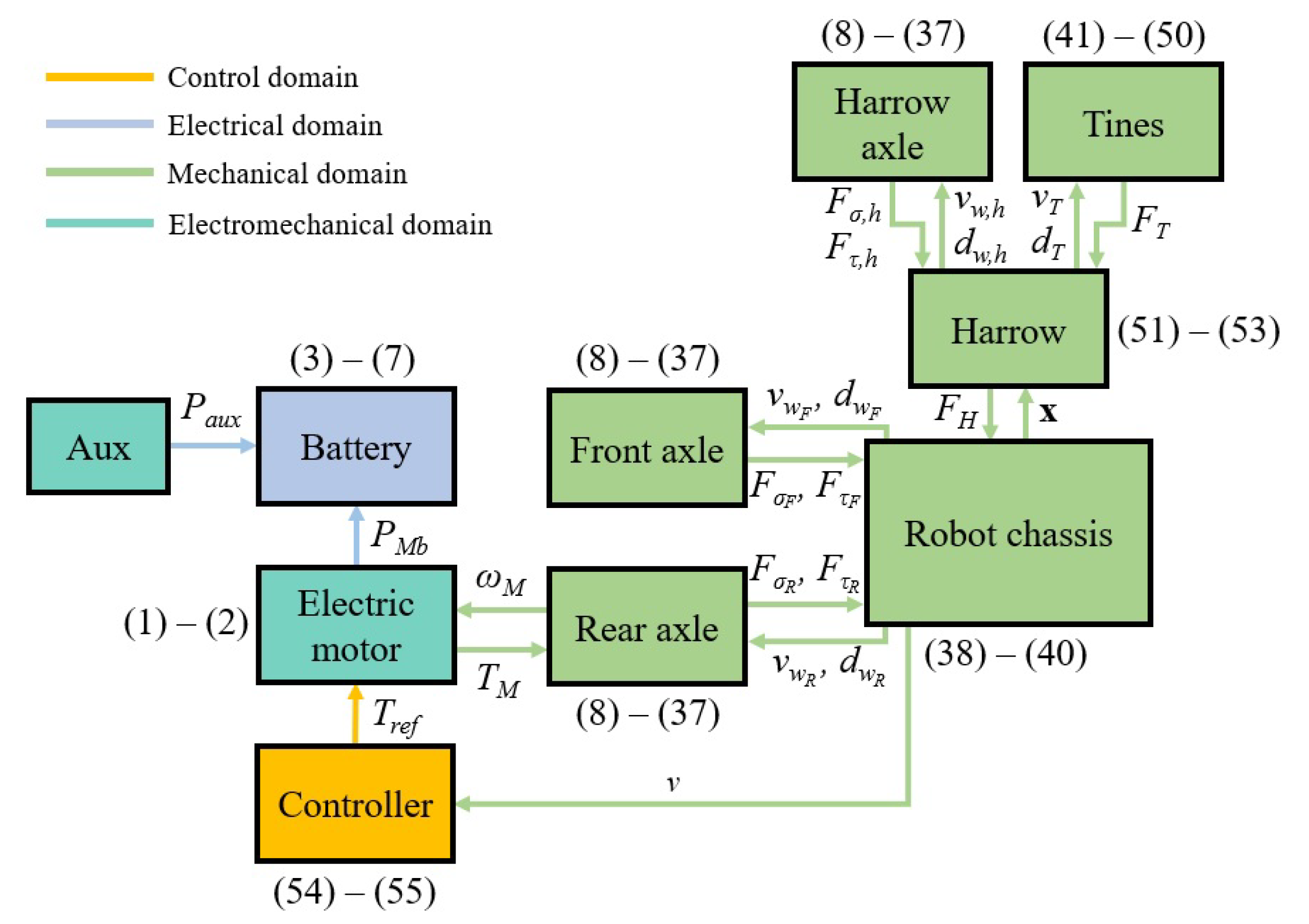

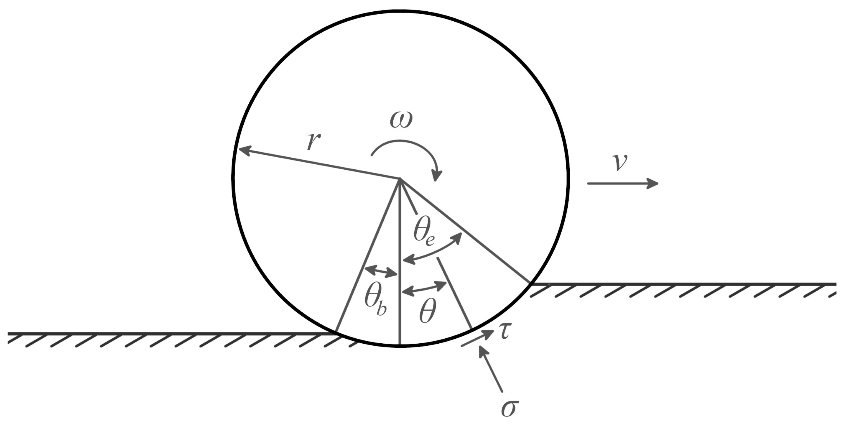

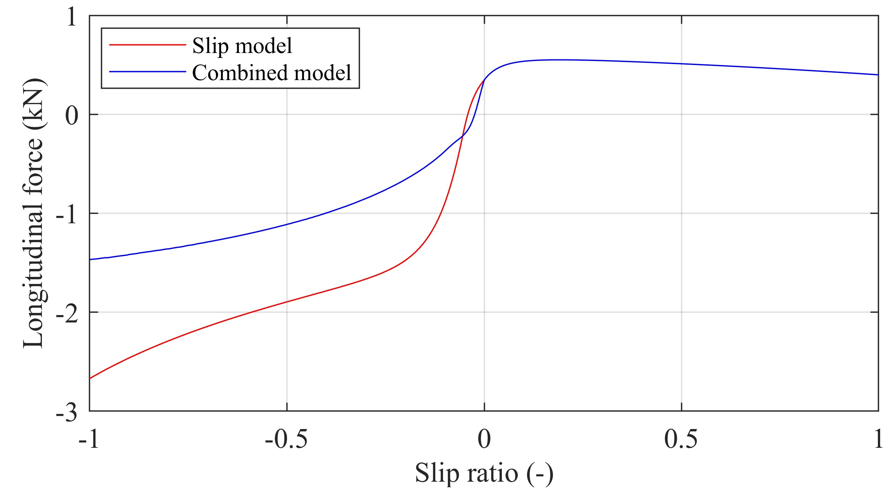
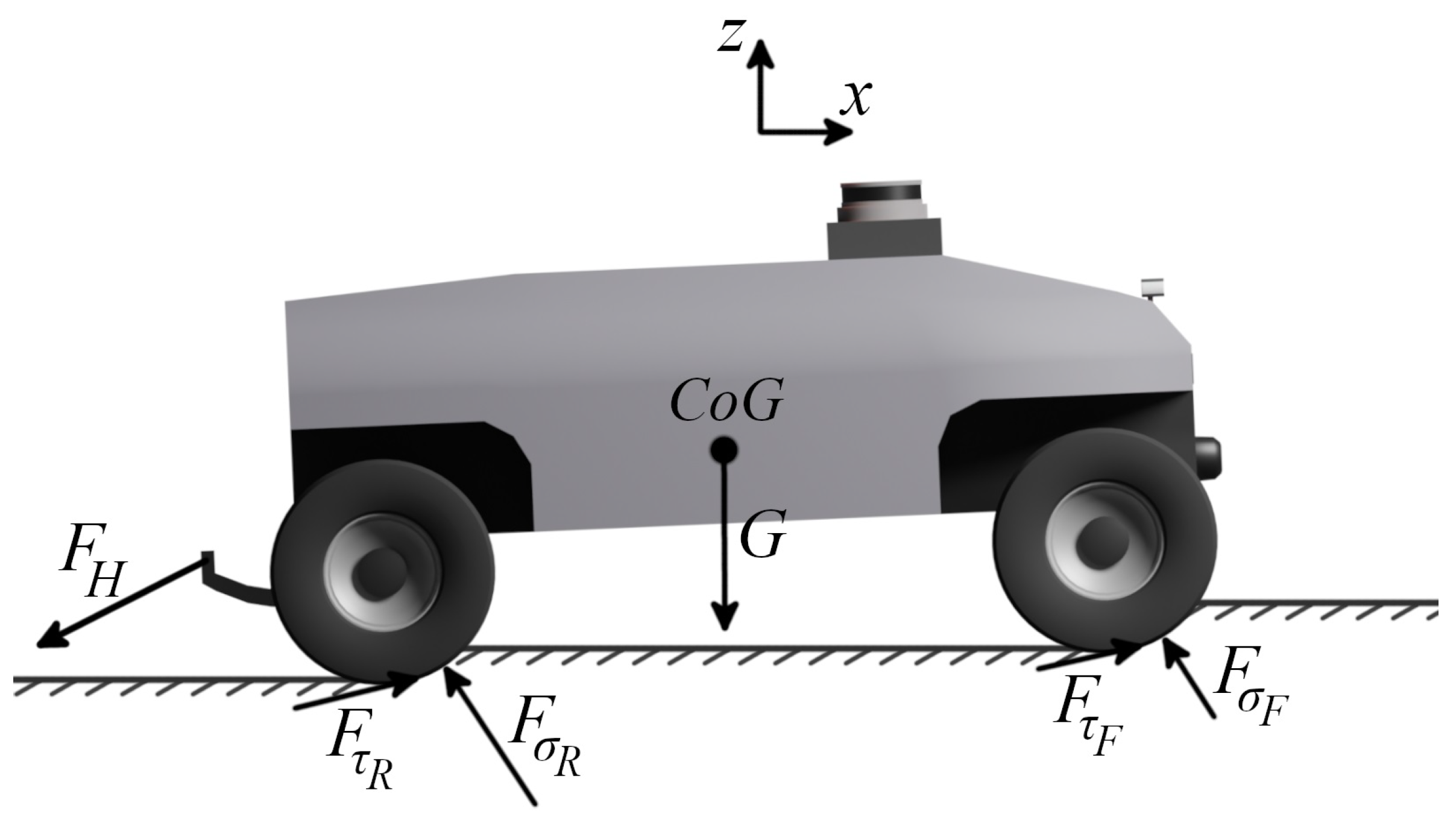


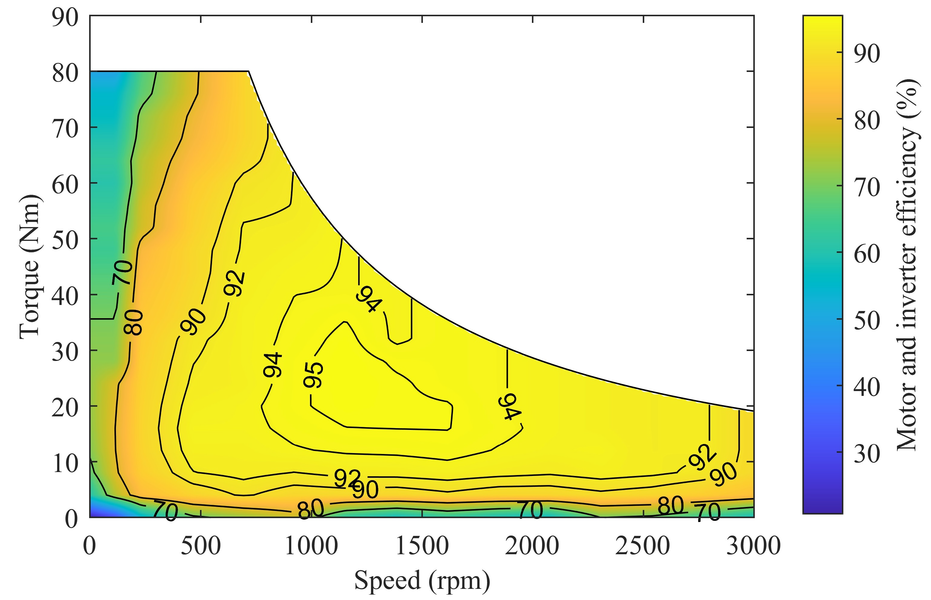
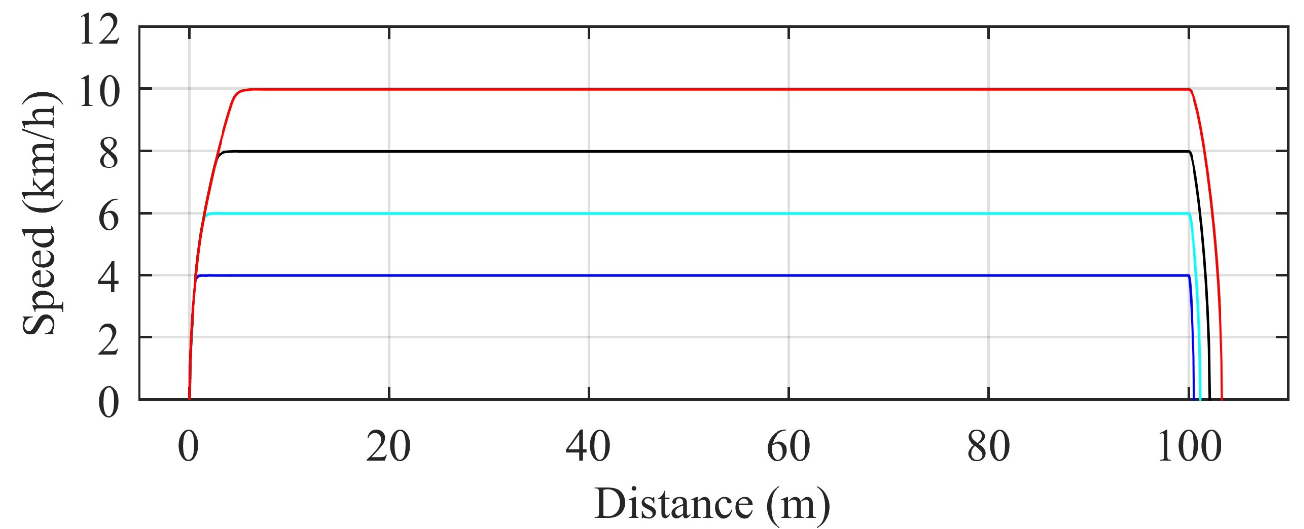
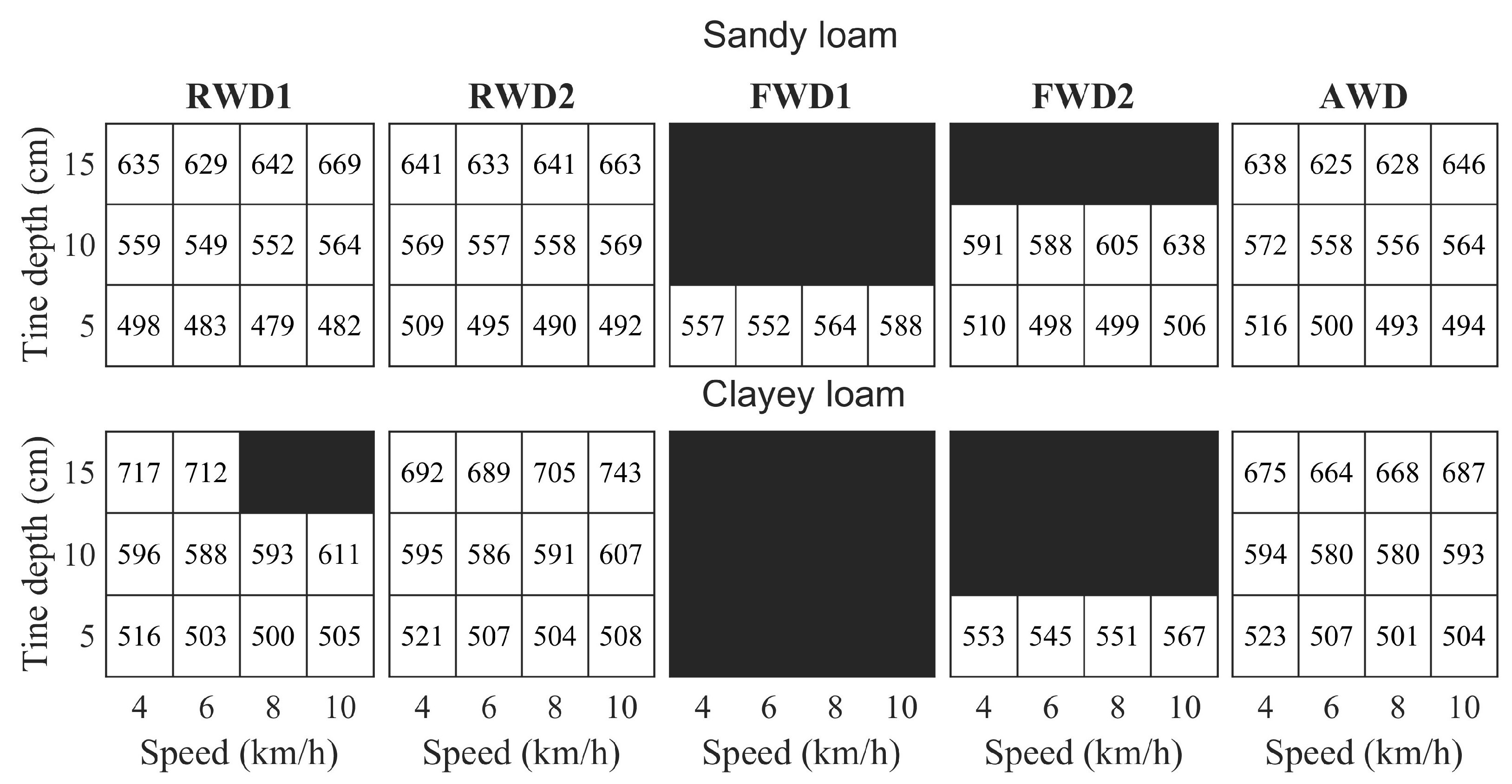
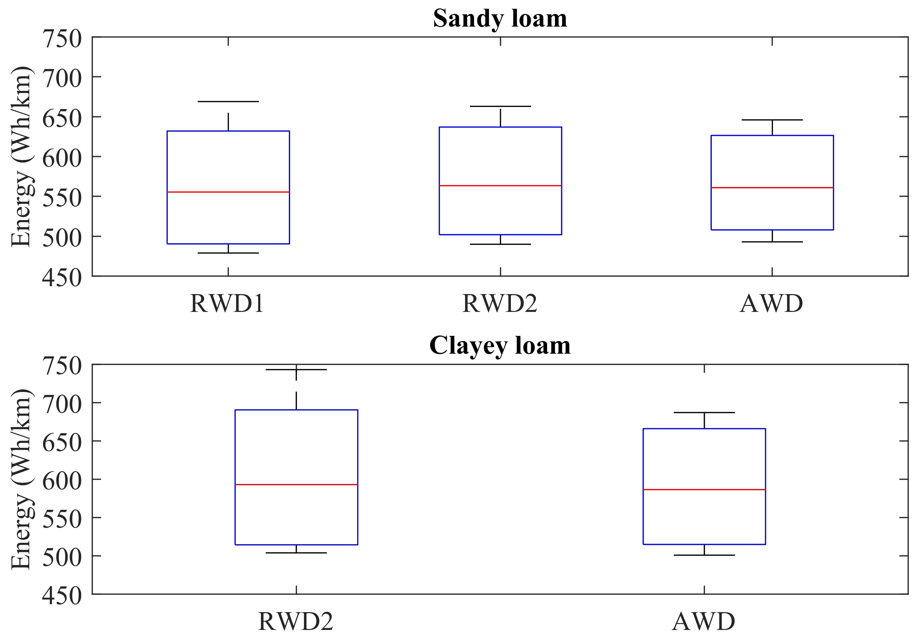
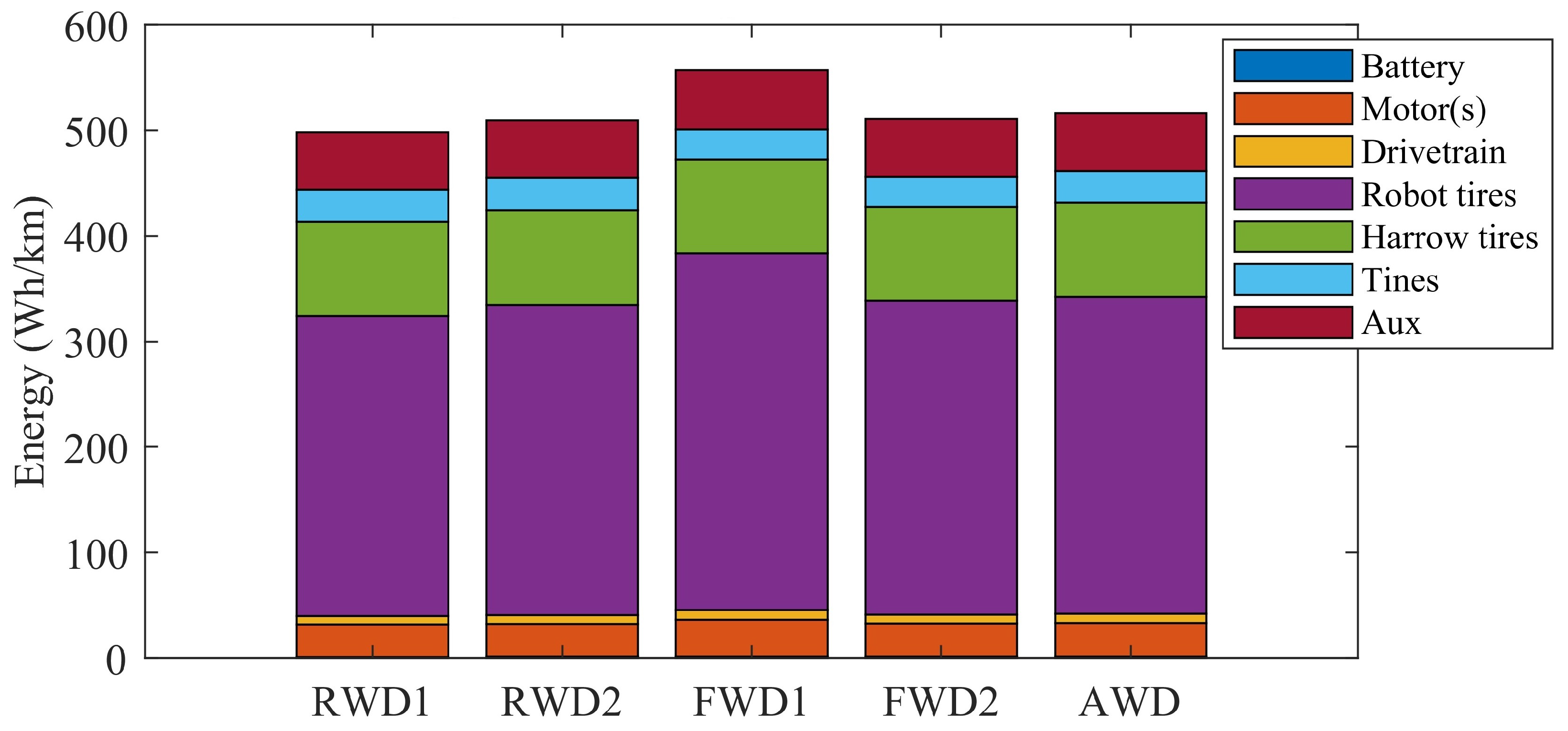
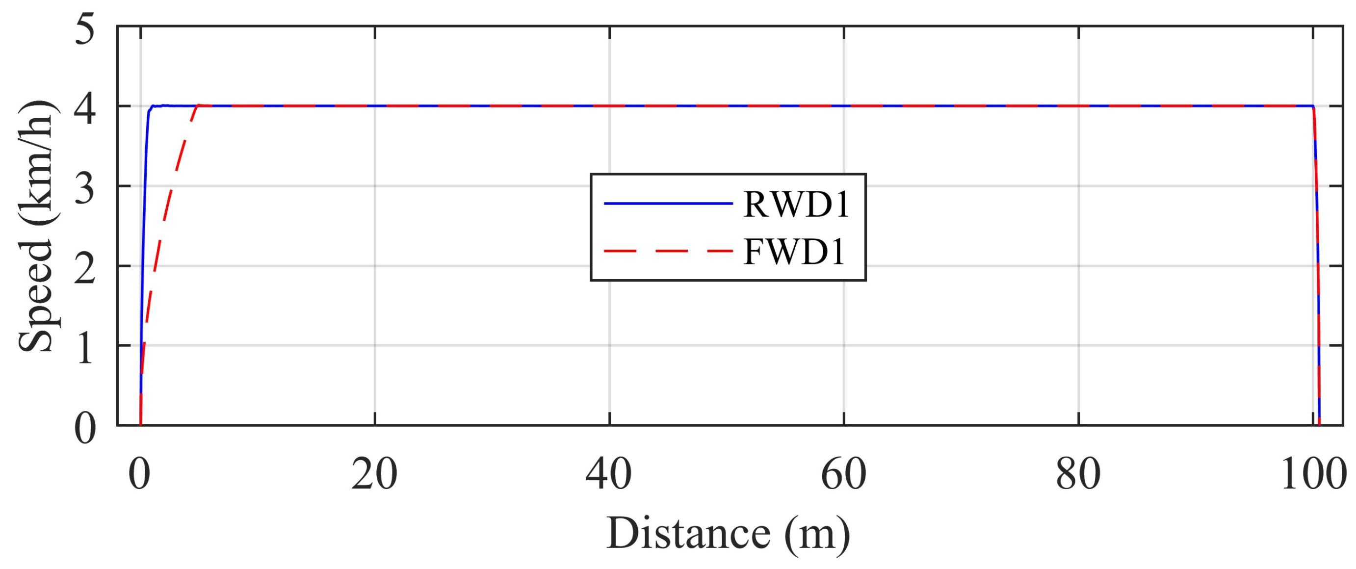
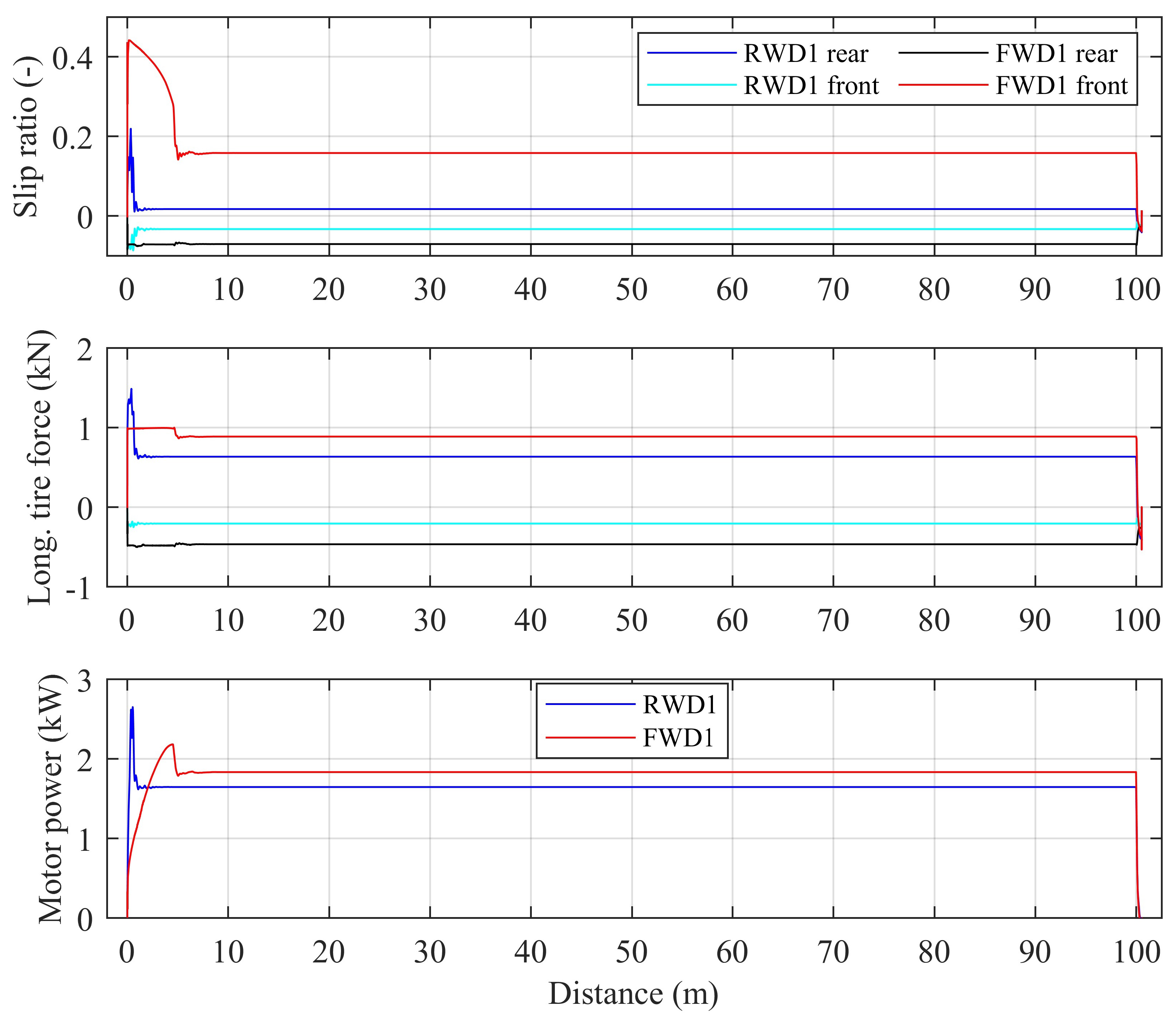
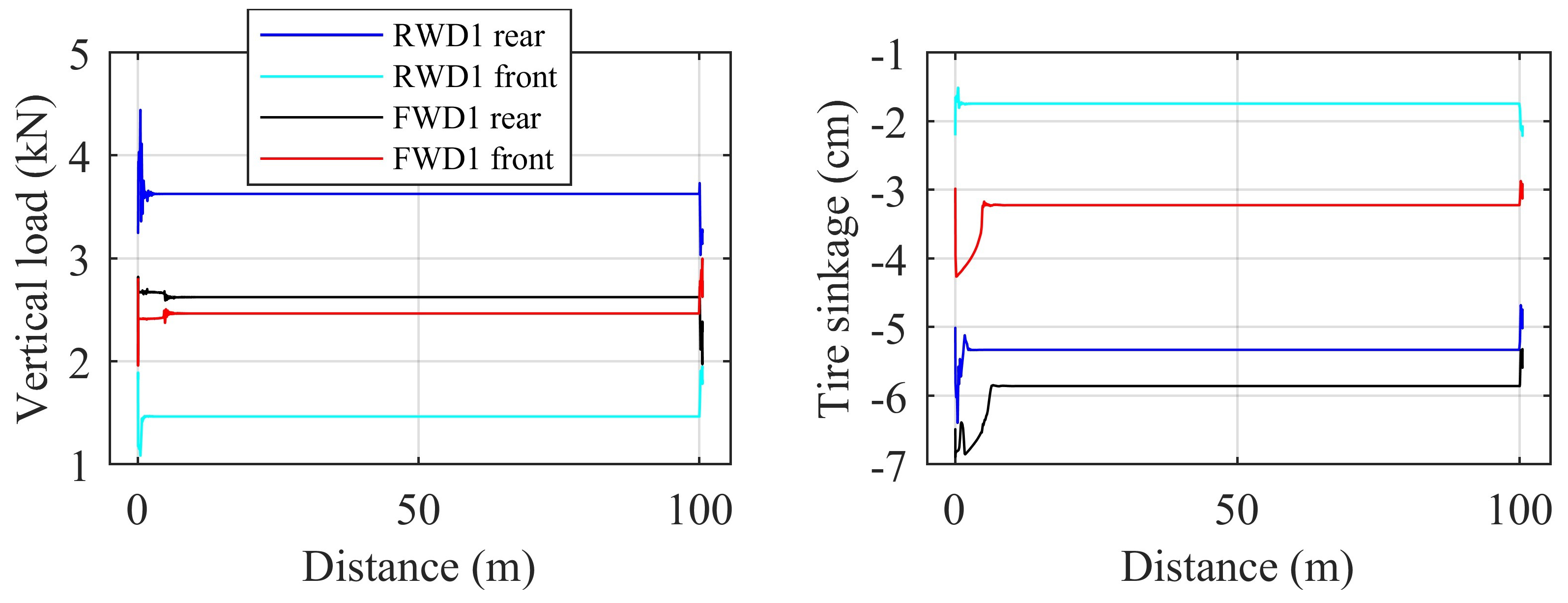
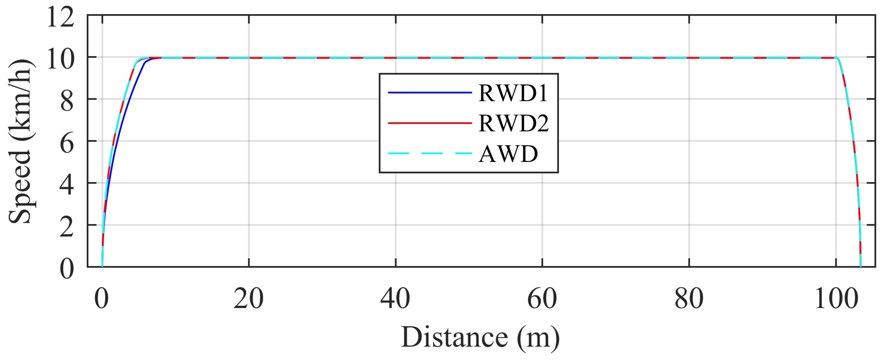
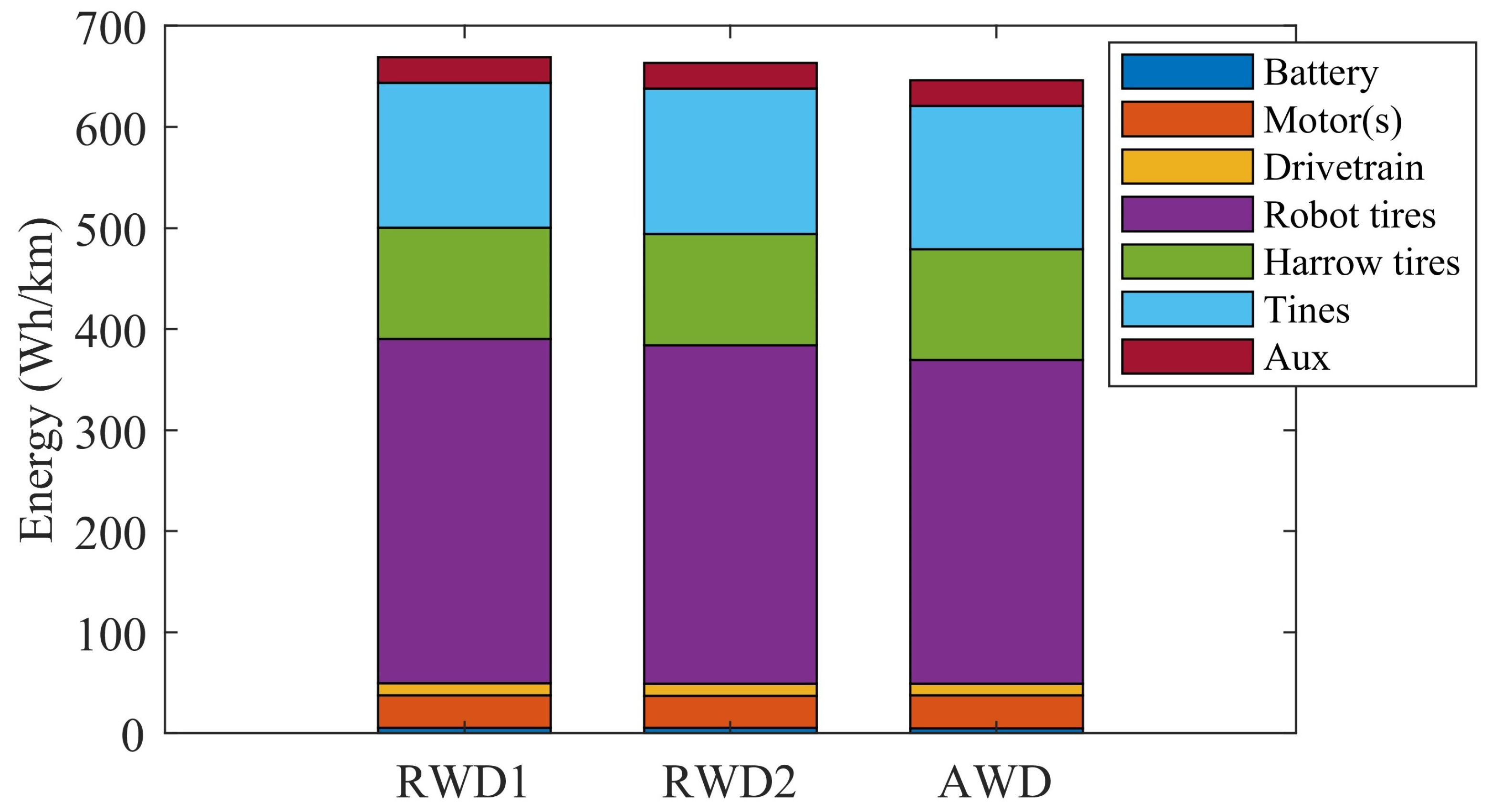
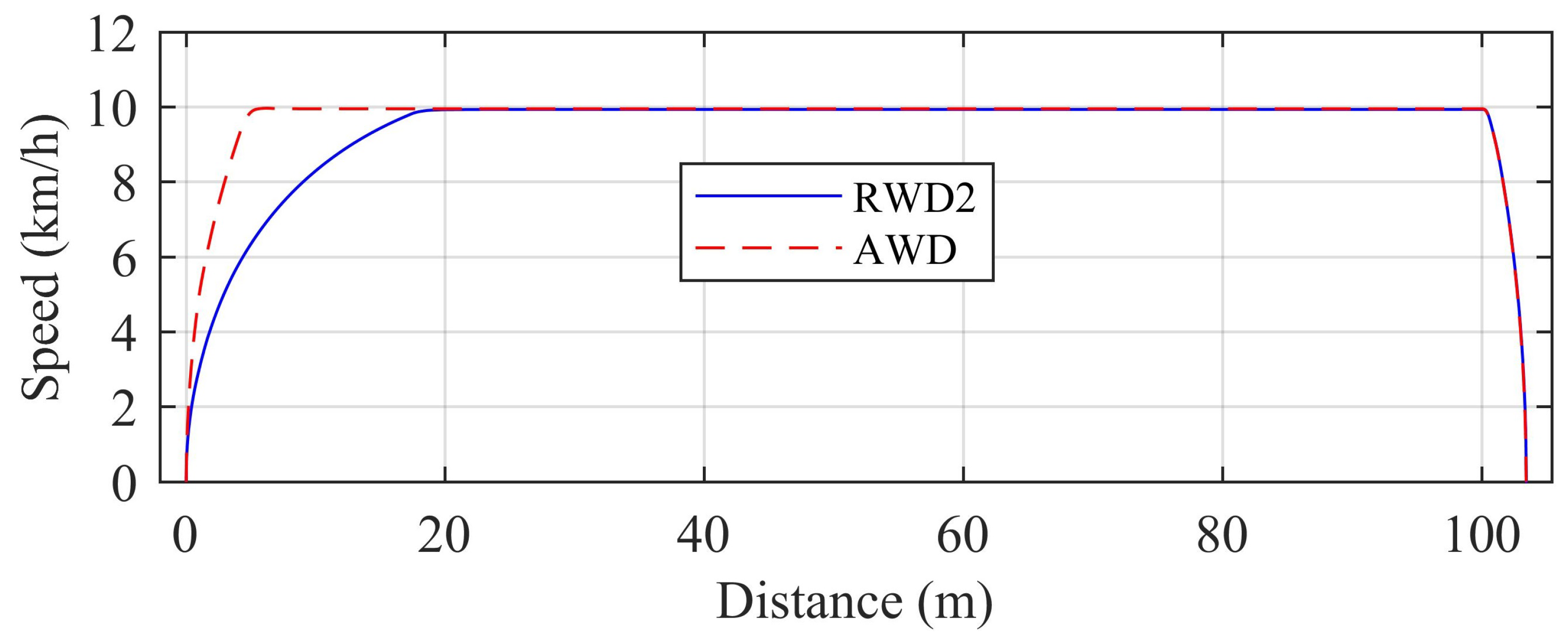
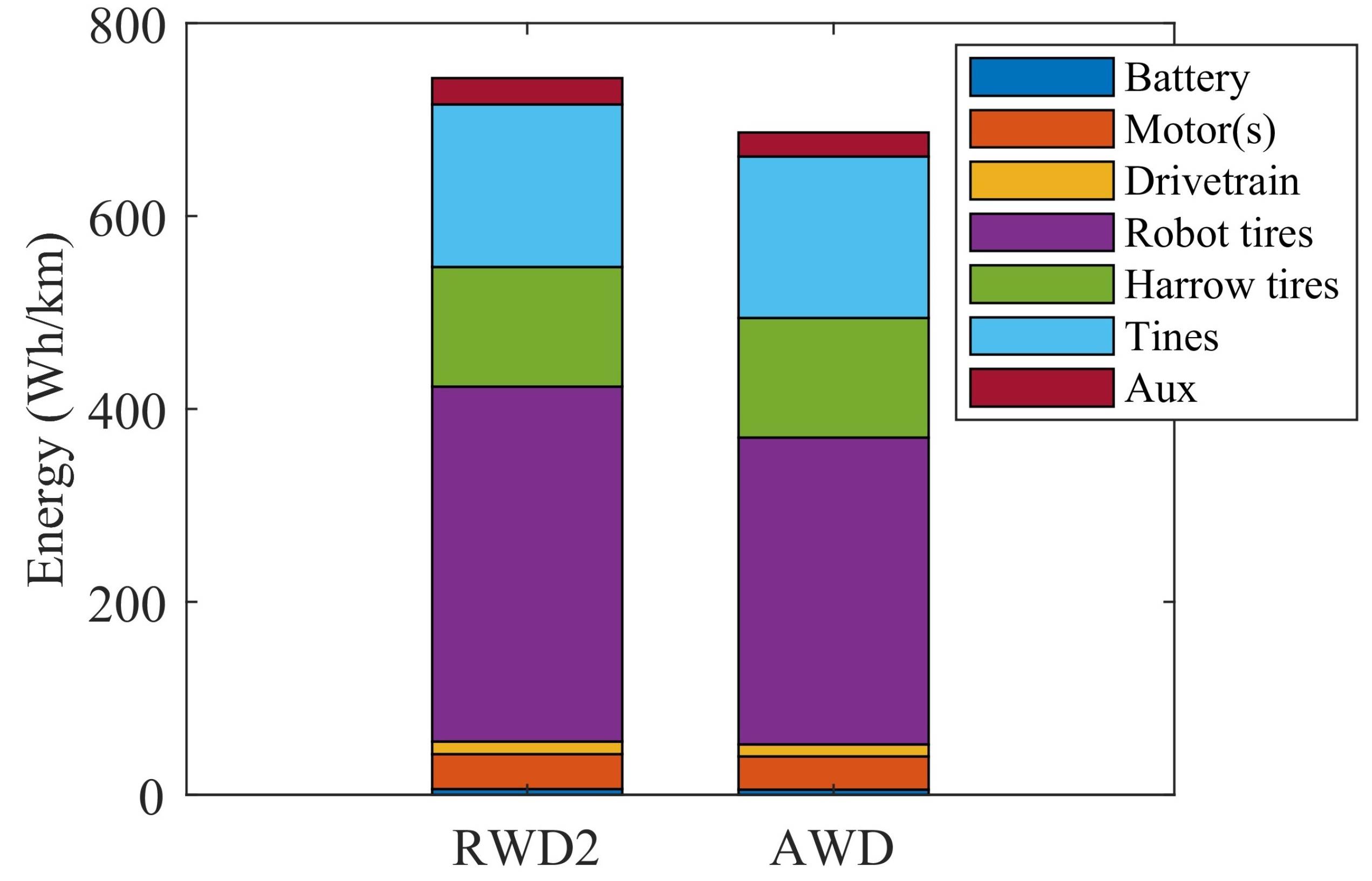
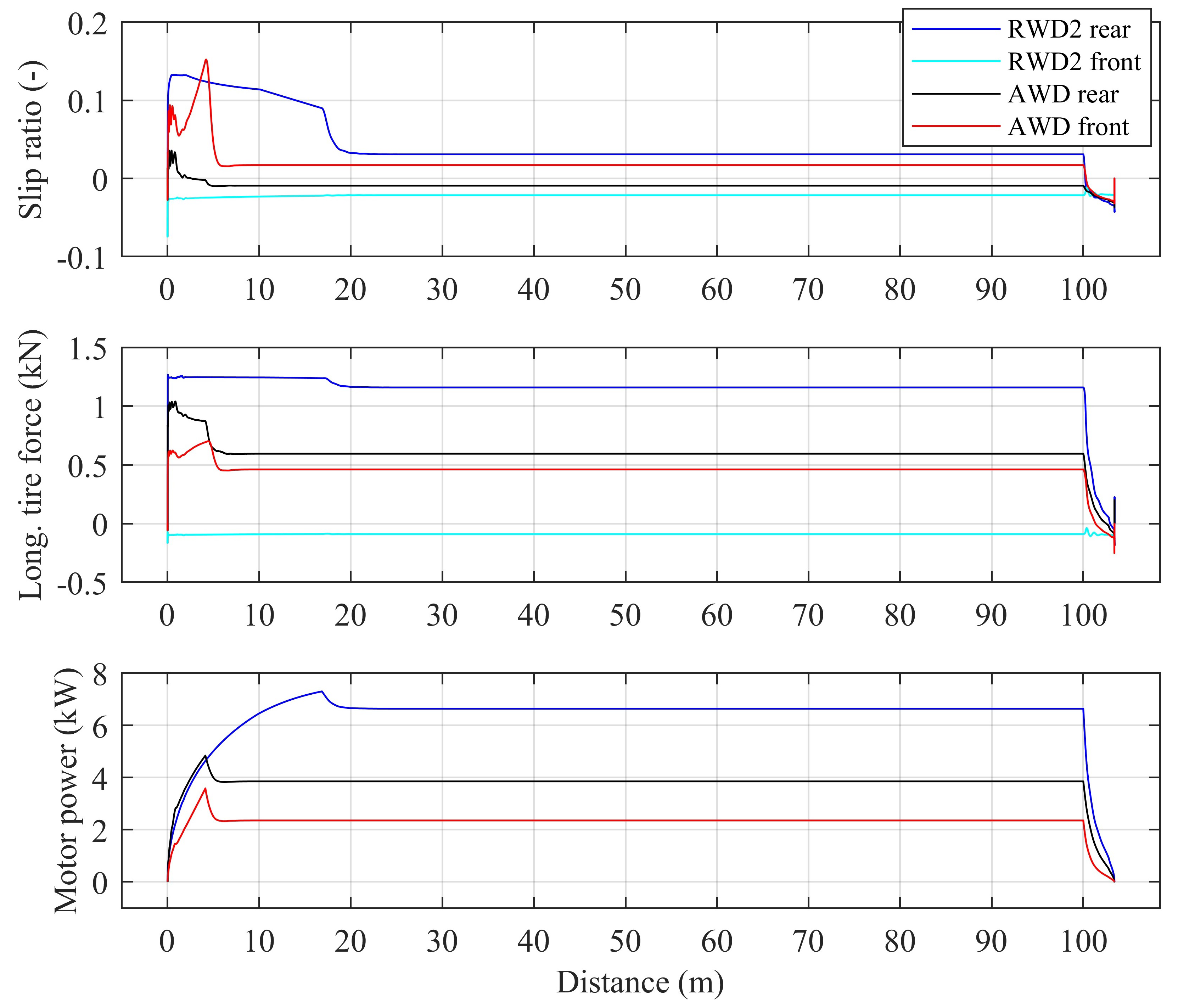

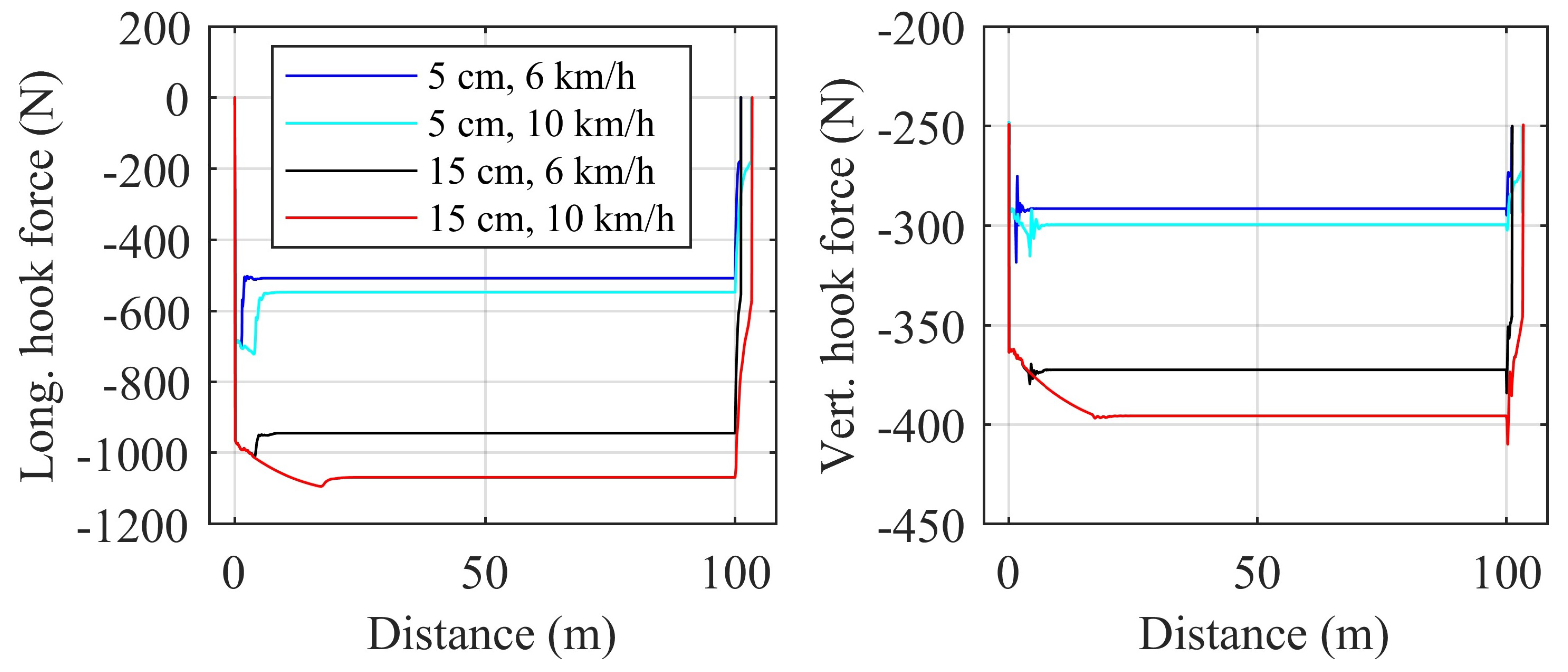
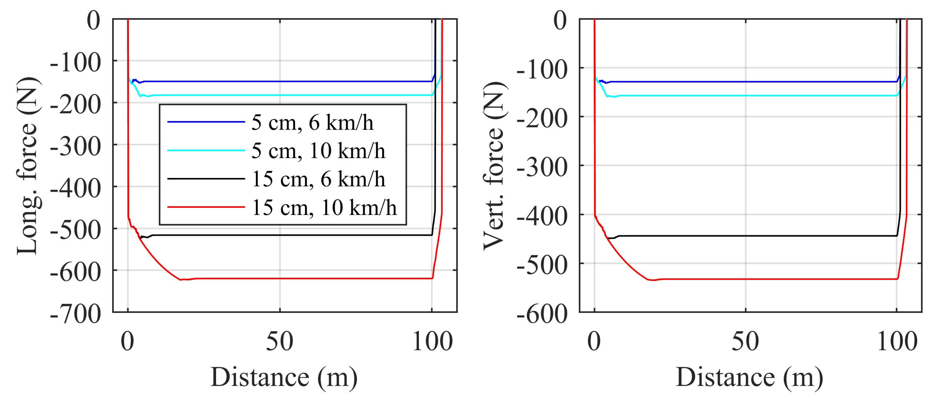
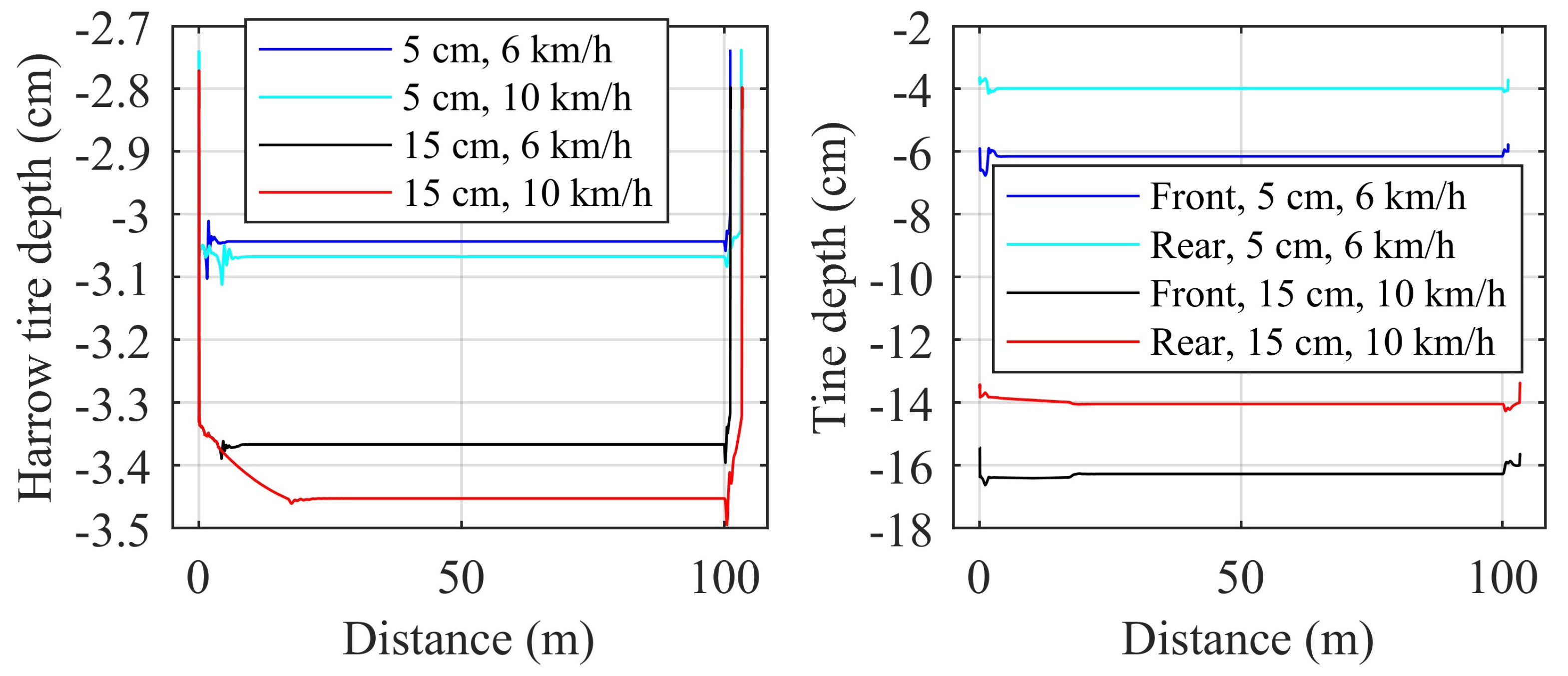
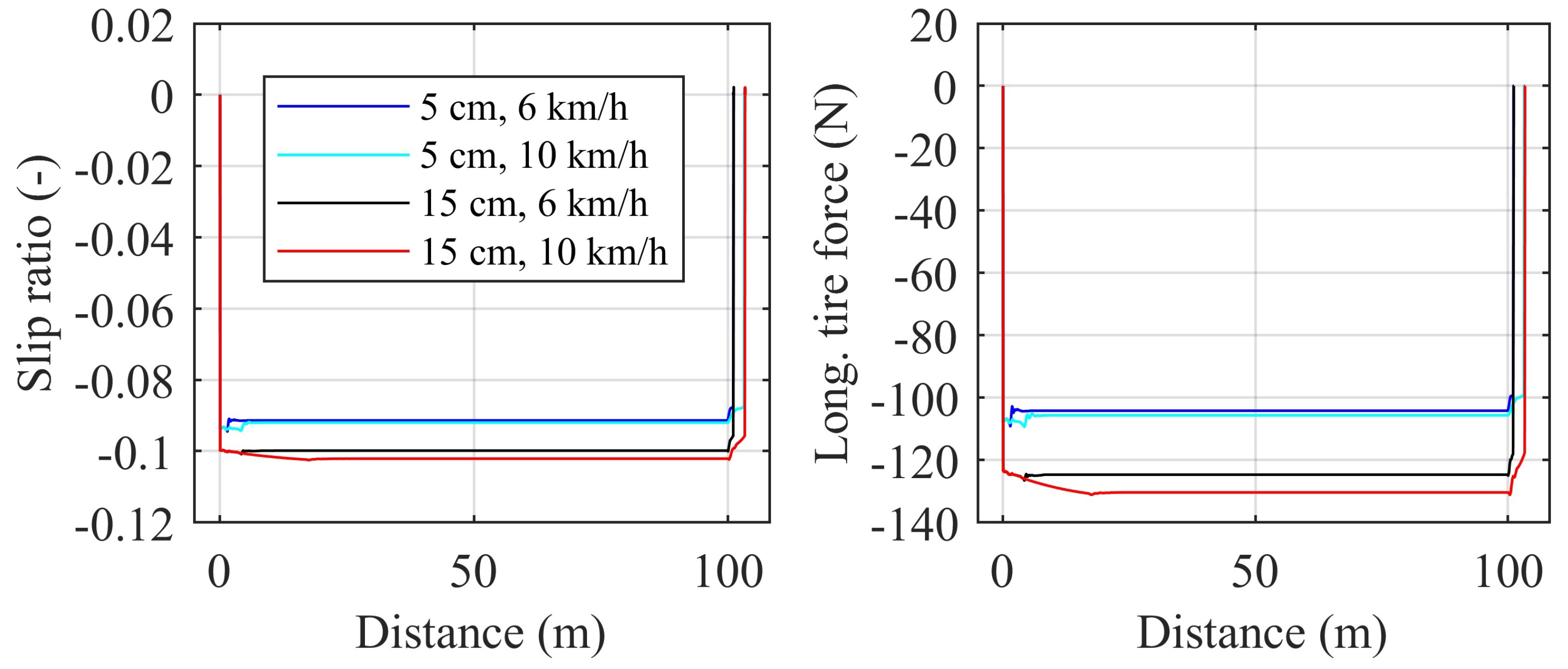
Disclaimer/Publisher’s Note: The statements, opinions and data contained in all publications are solely those of the individual author(s) and contributor(s) and not of MDPI and/or the editor(s). MDPI and/or the editor(s) disclaim responsibility for any injury to people or property resulting from any ideas, methods, instructions or products referred to in the content. |
© 2024 by the authors. Licensee MDPI, Basel, Switzerland. This article is an open access article distributed under the terms and conditions of the Creative Commons Attribution (CC BY) license (https://creativecommons.org/licenses/by/4.0/).