Abstract
Estimation of the region of attraction of the power system using sum of squares (SOS) programming theory is investigated in this paper. Firstly, the Taylor expansion formula is applied to explore the inherent polynomial structure of the swing equation. The single machine projection equation for a multi-machine system is proposed based on the amplitude characteristic of the rotor angle response in decoupled space. Secondly, the theory of SOS programming originating from the polynomial system is derived, and the theory about estimation of the region of attraction for the differential algebraic system is summarized. Thirdly, the method for estimating the region of attraction for the polynomial swing equation based on a V-S two-stage iterative procedure is proposed. Finally, a single machine infinite bus power system, an IEEE 3-machine power system, and an IEEE 4-machine power system are employed to validate the effectiveness and accuracy of the proposed method and analysis.
1. Introduction
Large-disturbance stability analysis of nonlinear systems has been a major challenge for a long time [1]. One reason is that the dynamic process of nonlinear systems is relatively complicated, while the other is a lack of effective mathematical tools. Historically, ever since Christiaan Huygens initiated the use of the scientific paradigm to study simple pendulums [2], the only tool available for theoretical analysis has been the law of conservation of energy, a status quo that persists to this day. Similarly, various analytical energy function methods have been proposed under the law of conservation of energy and Lyapunov’s second method [3,4] over the past years in the field of power system stability analysis. However, the systematic construction of an energy function with minimal model dependencies for stability analysis remains an open question [5] in the power system community.
In the past two decades, the connections among the SOS, algebraic geometry, and optimization have been discovered [6,7,8]. Hence, SOS programming theory has been systematically developed in response to Hilbert’s 17th mathematical problem in the sense of numerical optimization methodology [9]. The essence of the theory lies in its ability to verify the “positivity” condition of a polynomial via SOS programming, making it possible to construct Lyapunov functions for any polynomial dynamic system and enable the stability analysis for nonlinear systems, attracting extensive research attention.
A Lyapunov function search method based on SOS programming is proposed in [10], and corresponding examples are given to verify the effectiveness of the proposed method. Reference [11] also provides the construction method of the Lyapunov function for the differential algebraic equation (DAE) system based on SOS theory and gives an estimate of the domain of attraction. In [12], a local estimation method for the domain of attraction of the Van der Pol equation is proposed by combining SOS theory and simulations. Reference [13] enhanced the performance of the method for estimating the domain of attraction by introducing a shape factor based on the SOS theory, with this enhancement verified using the van der Pol equation and the second-order equation. To balance the trade-off between computation time and solution quality, the DSOS and SDSOS methods and their theoretical framework have been proposed and established based on algebraic geometry theory [14], which boosts the computational efficiency of the proposed methods. Driven by the demand for computing in large-scale systems, an approach has been proposed to address the significant increase in computation time associated with SOS optimization [15], aiming to estimate the domain of attraction for sparse polynomial differential systems in the event of computation burden. These results show the application potential of SOS in dealing with polynomial systems, something that has been extensively studied in various fields.
In the community of power systems, as renewable energy sources become integrated into the grid, the advantages of photovoltaic and other forms of generation are becoming increasingly apparent [16], leading to a greater emphasis on stability analysis methods. Thus, the SOS method has also attracted considerable attention. The potential of this method was first observed by Milano et al. [17], converting the power grid swing equations into a polynomial DAE system by introducing auxiliary variables; the estimation of the region of attraction for a three-machine power system is, thus, given. Using the same technique as Milano, reference [18] further gives the numerical energy function and calculation process of the power system in detail. In [19], addressing the computational burden associated with SOS optimization in large-scale power systems, a parallel and scalable algorithm is proposed to evaluate the stability of interconnected power systems using the Lyapunov function through the SOS method, with the corresponding adaptive and distributed control algorithms designed. In [20], by applying a multivariate Taylor expansion formula, non-polynomial power system equations are transformed into uncertain DAE. The SOS method and squared matrix representation are then employed to find the optimal fractional-type Lyapunov functions for the system, and an estimation of the domain of attraction for the equation is provided. In [21,22], the problem of system security domain with low voltage ride through is defined as an SOS programming problem within the context of the DAE system framework, and a systematic solution is presented. Reference [23] uses the SOS programming method to analyze the robust stability of power systems with uncertain parameters, extending the application of the SOS method. Reference [24] focuses on the phase-locked loop equations in power system converters, and the comparisons with time-domain simulations and hardware-in-the-loop experiments results validate the accuracy of the estimation of domain of attraction based on the SOS method. However, the technique mentioned above in the multi-machine scenario converting the non-polynomial swing equations into polynomial dynamical systems is based on the introduction of auxiliary variables, increasing the dimension of the equation and destroying the intrinsic structural characteristics of the original equation.
Hence, this paper investigates the estimation of the domain of attraction for power systems by adopting a rather different approach: exploring the inherent polynomial structural characteristics of the swing equation without introducing auxiliary variables. Specifically, the Taylor formula is used to reveal the inherent polynomial structure of the swing equation both in single machine and multi-machine scenarios, which establish the polynomial model of the power grid dynamic equation in general. Subsequently, the method to estimate the region of attraction for polynomial power systems based on V-S two-stage is proposed. Finally, the simulation examples from a single-machine infinite bus power system, IEEE 3-machine 9-bus system, and IEEE 4-machine power system demonstrate the effectiveness of the proposed method.
2. Theoretical Basis of SOS
In this section, the theoretical basis of SOS is reviewed. Specifically, the basic concepts in algebraic geometry and the key theorem are presented in Section 2.1 and Section 2.2, respectively; more details can be found in reference [6].
2.1. Basic Concepts
This section introduces some key concepts in algebraic geometry and SOS programing theory. Three basic concepts are introduced as follows,
Definition 1 (monomial).
The monomials for variables are defined as follows,
where is a monomial. The degree of the monomial is defined as follows,
Definition 2 (polynomial).
The polynomial for variables is defined as follows,
The degree for the polynomial is defined as,
The set of all variables polynomials is defined as follows,
All sets of degree not exceeding in the definition of are as follows,
The dimensions polynomial vector is defined as follows,
The set of SOS for variables is defined as follows,
where all set of degree not exceeding in the definition of are denoted as follows,
2.2. Key Result
This section introduces the key result in SOS theory. Three basic concepts are demonstrated as follows,
Definition 3 (Monoid).
Given , a monoid is defined as follows,
Definition 4 (Cone).
Given , a cone is defined as follows,
Definition 5 (Ideal).
Given , an ideal is defined as follows,
Theorem 1 (Positivestellensatz).
Given the subset , , and in , the following two conditions are equivalent,
1. The following subset is empty,
2. There exists , , and such that the following equation is satisfied,
3. The Polynomial Model of Power Systems
In this section, the polynomial model of the power system in single-machine and multi-machine scenarios is derived. Specifically, the polynomial model of the single-machine system is obtained in Section 3.1, and the projection polynomial equation for the multi-machine system is derived stepwise in Section 3.2.
3.1. Polynomial Model of Single-Machine Systems
Consider the equation of a single-machine infinite bus power system as follows,
The Taylor expansion formula is adopted as follows,
Substituting Equation (16) into Equation (15), we obtain the following equation,
Shifting the equilibrium point of Equation (17) to the origin by introducing the coordinate transformation , where is the stable equilibrium point of Equation (15), Equation (17) can be written as,
where , , and the coefficients in Equation (18) are shown as follows,
3.2. Polynomial Model of Multi-Machine Systems
In the case of multi-machine systemss, when the generator adopts a constant voltage model after transient reactance and the load adopts a constant impedance model, the dynamic process after a large disturbance can be described by the initial value problem [25], as demonstrated in Equation (20),
where represents the rotor angle difference, indicates the number of synchronous machines in the power grid, is the reference frequency of the power grid, represents the mechanical power of the i-th machine, and represents the initial values of the state variables. The other coefficients in Equation (20) are defined as follows,
where represents the elements of a complex admittance matrix in a reduced network related to the power grid, and is the potential behind the transient reactance of the i-th machine.
Using the same technique as in Equation (16), the swing Equation (20) can be rewritten as follows when the sine function is expanded to a cubic term,
where is the coefficient. We move the stable equilibrium of Equation (22), i.e., , into the original by applying the coordinate transformation . Hence, the right-hand side of Equation (22) can be expressed as follows,
where and . In order to write the algebraic Equation (23) in matrix form, the following coefficient matrix P is defined,
where indicates the angle difference. Hence, the matrix form of Equation (23) can be represented as follows,
where and are the inertial matrix and damping matrix, respectively. is the coefficient matrix corresponding to Equation (23). Specifically, can be written as follows,
Notice that the matrix in Equation (24) has some structural characteristics because of the constraint imposed by Equation (24). Without loss of generality, we take n = 3 as an example to illustrate the structural characteristics of P as follows:
It can be seen that , which means that the summation of any row of P is equal to 0. Hence, we introduce a linear transformation satisfying the following,
where are the nonzero eigenvalues of the matrix . Considering the characteristics of matrix P, we have . Thus, by substituting Equation (28) and eigen-transformation into Equation (25), we obtain a partly decoupled polynomial mode of swing equation as follows,
where , , , and . Assuming that there is uniform damping in the power system [26], i.e., , Equation (29) can be written as follows,
It becomes obvious that the main subsystem (30)-(a) is completely decoupled from the variable , and the system (30)-(b) completely depends on the main subsystem variable . It is pleasant to observe that the above two systems can be solved sequentially. Therefore, the description of the transient stability problem in the power system can be formulated as the initial value problem of a second-order polynomial nonlinear state–output equation, as shown in Equation (31),
where the state variable and the nonlinear function are polynomial mappings, specifically, , , .
3.3. Single-Machine Projection Polynomial Equation for Multi-Machine Systems
In the coordinate system in Equation (31), the equation describing the motion of the maximum rotor angle is given as follows,
where represents the M-th row of the matrix , and the symbol represents the Hadamard product of matrices. Denoting the variable , the quadratic term in Equation (32) can be demonstrated as follows,
where the subscript M indicates the maximum value term, subscript c represents the coupling term, and subscript o represents other terms. The cubic term in Equation (32) can be reformulated as follows,
where the meaning of the different subscripts is the same as in Equation (33). Therefore, combining Equations (33) and (34), the equation describing the motion of the maximum rotor angle in Equation (32) can be rewritten as follows,
It is obvious that the forces governing the variation of maximum rotor angle can be decomposed into eight parts from Equation (35). Specifically, these forces can be divided into three categories, i.e., self -terms (, , ), cross-coupling terms (, , ), and other terms (, ).
It is observed that there are response characteristics in the coordinate system which can be spotted in the section of cases studied. Hence, this allows the formulation of the following equation,
Thus, Equation (35) can be approximated as follows,
where . Therefore, the single-machine projection equation in the multi-machine scenario is obtained, with the physical significance of reducing a coupled multi-machine equation to a single-machine equation describing the motion of the maximum rotor angle.
4. Estimation of the Region of Attraction Method in Power Systems
In this section, the fundamental theory of the region of attraction is reviewed (Section 4.1), and the methods and procedures for estimating the region of attraction of power systems is proposed (Section 4.2).
4.1. Fundamental Theory
Consider a polynomial-type constrained DAE as follows,
where , namely , , and , represent polynomial systems. Let the origin be a stable equilibrium point in Equation (38) and let us denote the solutions satisfying Equation (38) with the initial condition by . The definition [1] and key theorem associated with the domain of attraction are introduced as follows,
Theorem 2 (Extended Lyapunov Theorem [27]).
For the given DAE system represented by Equation (38)-(a), if there exists a set containing the origin, and there exists a smooth function , with , such that the following inequality (40) holds,
where is a known function, then the system described by Equation (38)-(a) is asymptotically stable at the origin.
Considering the constrained DAE (38), and assuming the existence of a known function , if there exists a polynomial-type function , i.e., , satisfying the conditions based on inequality (41),
Equivalently, the set operation form is obtained combing Equation (40) with Equation (41) as follows,
Formula is defined to represent the constraint in Equation (42), where indicates a small parameter. Hence, the empty set form of Equation (42) can be written as follows,
Define the set , and can represent an estimate of . Based on Theorem 1 and the equivalent conditions in Equation (43), the estimation of the region of attraction can be formulated in the form of an SOS programming problem as follows,
4.2. Methods and Procedures for Estimating the Region of Attraction of Power Systems
Considering the model of the power system as pure differential equations, the estimation of the region of attraction of Equations (18) and (37) in single-machine and multi-machines scenarios, respectively, can be written as follows according to Equation (44),
To reduce the complexity of the optimization model mentioned above, we set . Considering the nonlinear relationship between the decision variables and , to simplify the planning problem we set . Notice that , therefore, the formular and the following equation are formulated,
Therefore, the optimization problem described by Equation (45) can be formulated as a quadratic programming form as follows,
Given that the decision variables and in Equation (47) exhibit bilinear characteristics, which are generally difficult to solve, the decision variables are fixed separately and the bilinear optimization of Equation (47) is divided into two sub-problems and two stages of optimization problems as follows,
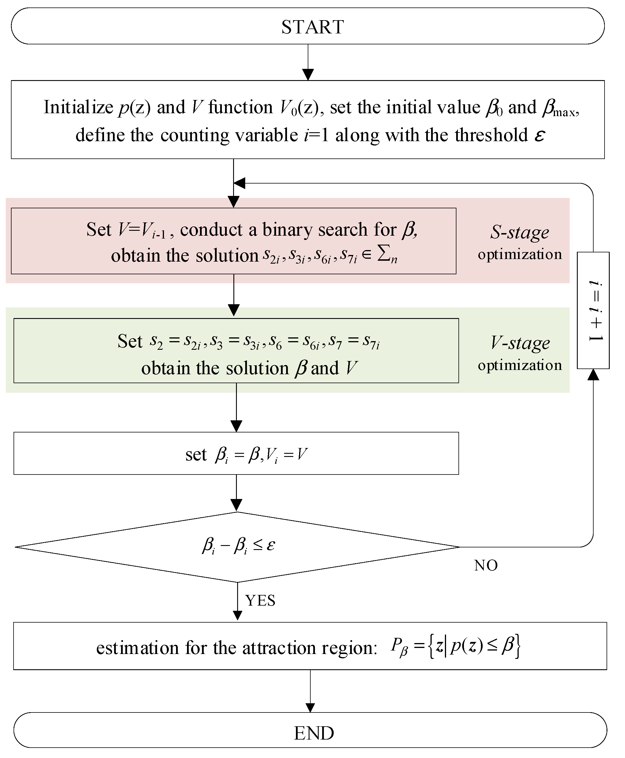
Therefore, the procedure to estimate the region of attraction based on Equation (48) can be summarize as shown in Figure 1.

Figure 1.
Procedures behind the estimation of the region of attraction.
5. Case Study
In this section, several power system examples are employed to show the effectiveness of the proposed method.
5.1. Single-Machine Infinite Bus System
Consider a single-machine infinite bus system with the system parameters as described in Table 1 and the topology as shown in Figure 2.

Table 1.
Parameters of single-machine infinite power system.
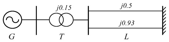
Figure 2.
Single-machine infinite power system.
According to the technique described in Section 3.1 with the aid of parameters in Table 1, the polynomial model of a single-machine infinite power system, originating from the swing equation, can be obtained as follows,
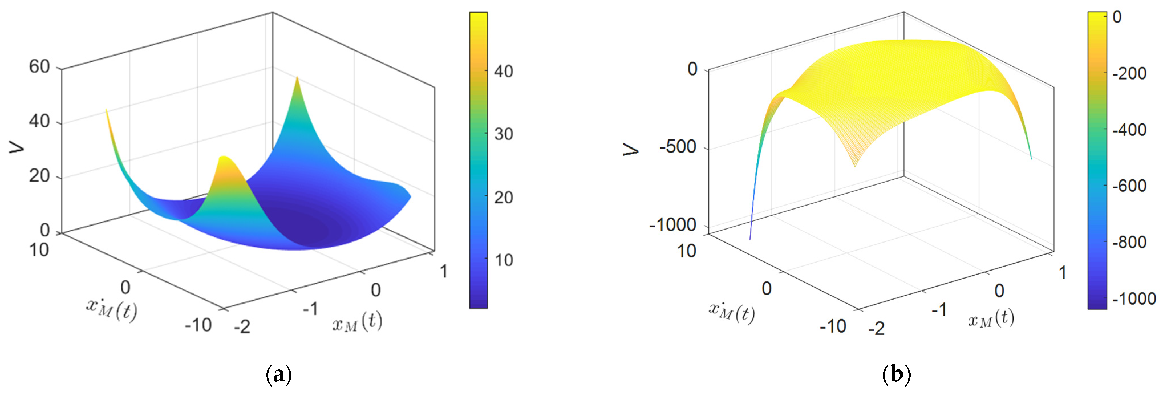
Once the polynomial mathematical model Equation (49) is obtained, the SOS programming method can be used to compute the eligible V-function, which has a distribution of values in (δ, ω) space as shown in Figure 3 below.
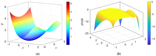
Figure 3.
Value distribution of the V function and its derivative. (a) Value distribution of the V function; (b) value distribution of the derivative of the V function.
In Figure 3a, it can be observed that the V function is positive in a large area near the origin, while it is always negative near the origin for the derivative of the obtained V function. This confirms that the V function obtained by the SOS method satisfies the two conditions imposed by Equation (40), meaning that the V function is a candidate function from Theorem 2. Moreover, the domain of attraction of the single-machine system is plotted using this V function as shown in Figure 4.
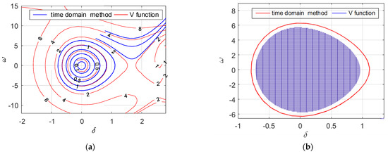
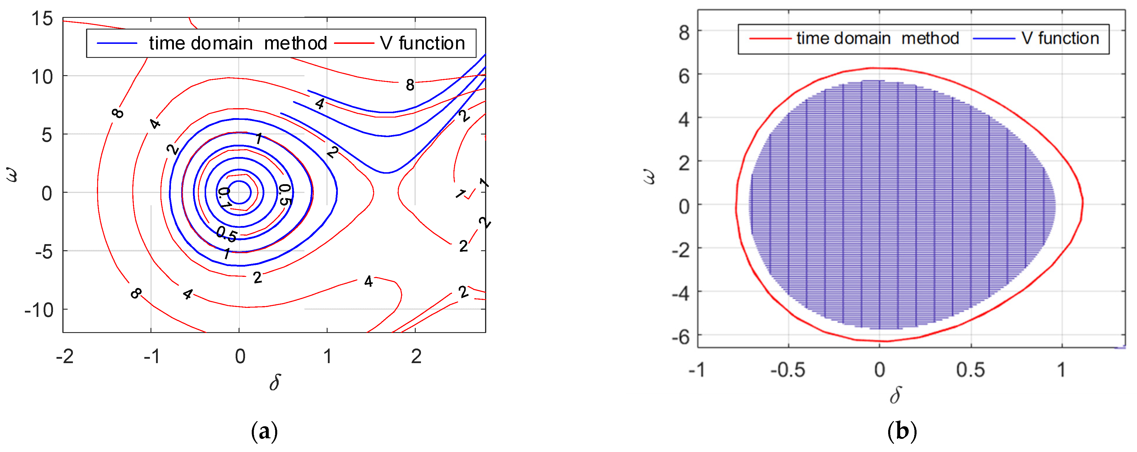
Figure 4.
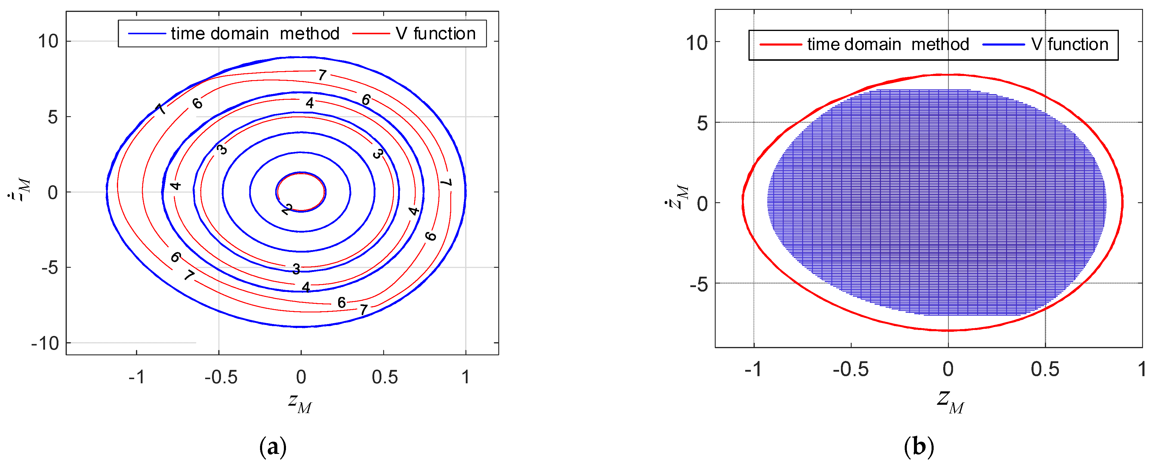
Comparison diagram for the estimation of the domain of attraction of single-machine infinite bus system. (a) Contour of the domain of attraction; (b) comparison with the time-domain method.
It can be observed from Figure 4 that there is a considerable overlap between the domain of attraction generated by the V function and the phase portrait, respectively, confirming the validity of the estimation method detailed in Section 4. Furthermore, the time-domain simulation result in and out of the domain of attraction, i.e., , is shown in Figure 5.
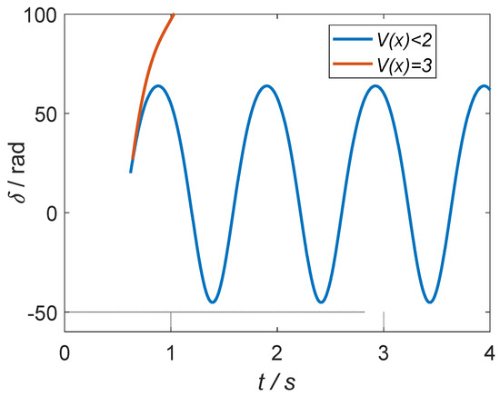
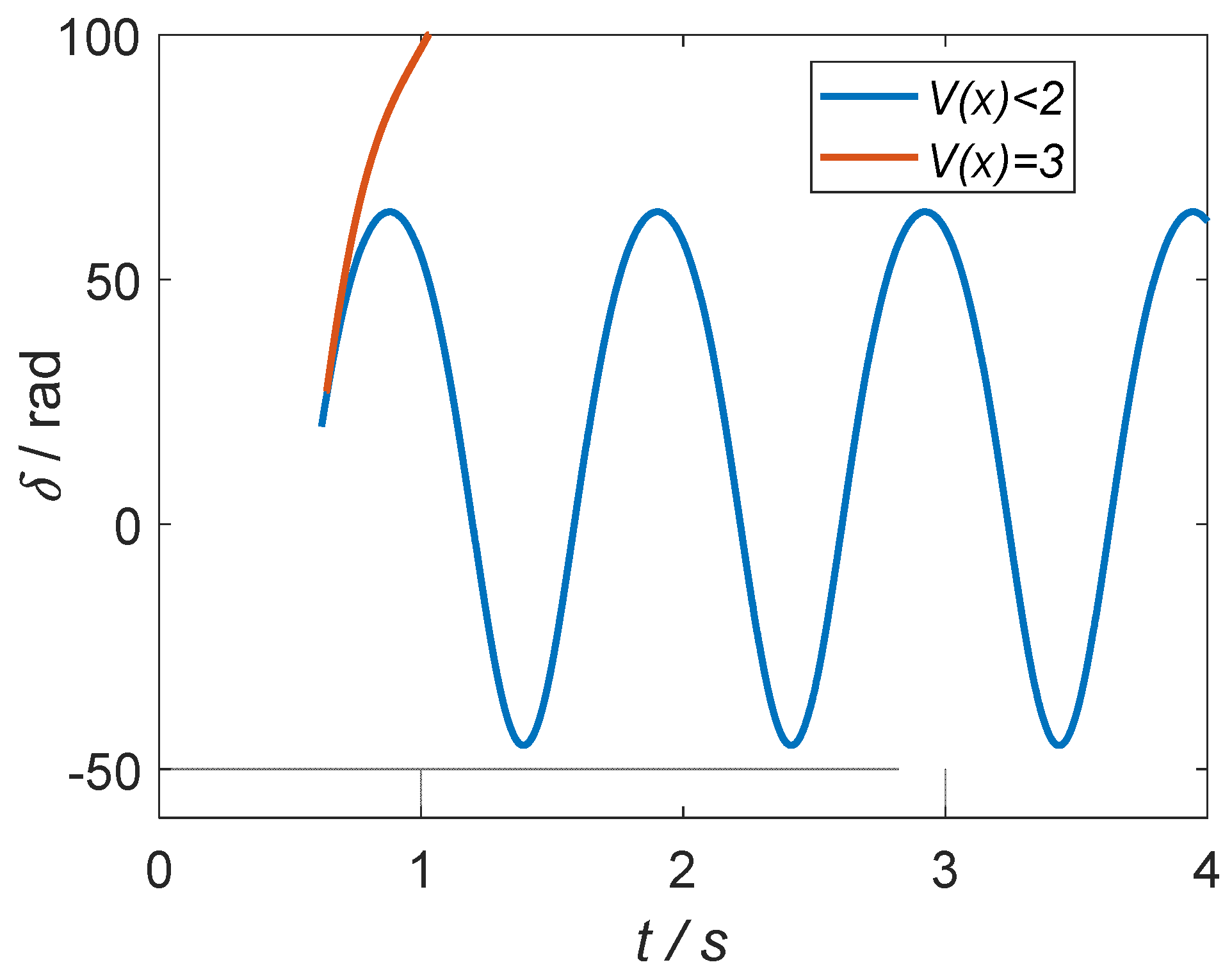
Figure 5.
Time-domain simulation curves.
It can be noticed from Figure 5 that the rotor angle outside the estimation of the region of attraction diverges, while the rotor angle is stable when the initial value is in the estimation of the region of attraction. This verifies the validity of the method proposed in this paper for the estimation of the domain of attraction.
5.2. IEEE 3-Machine Test Power System
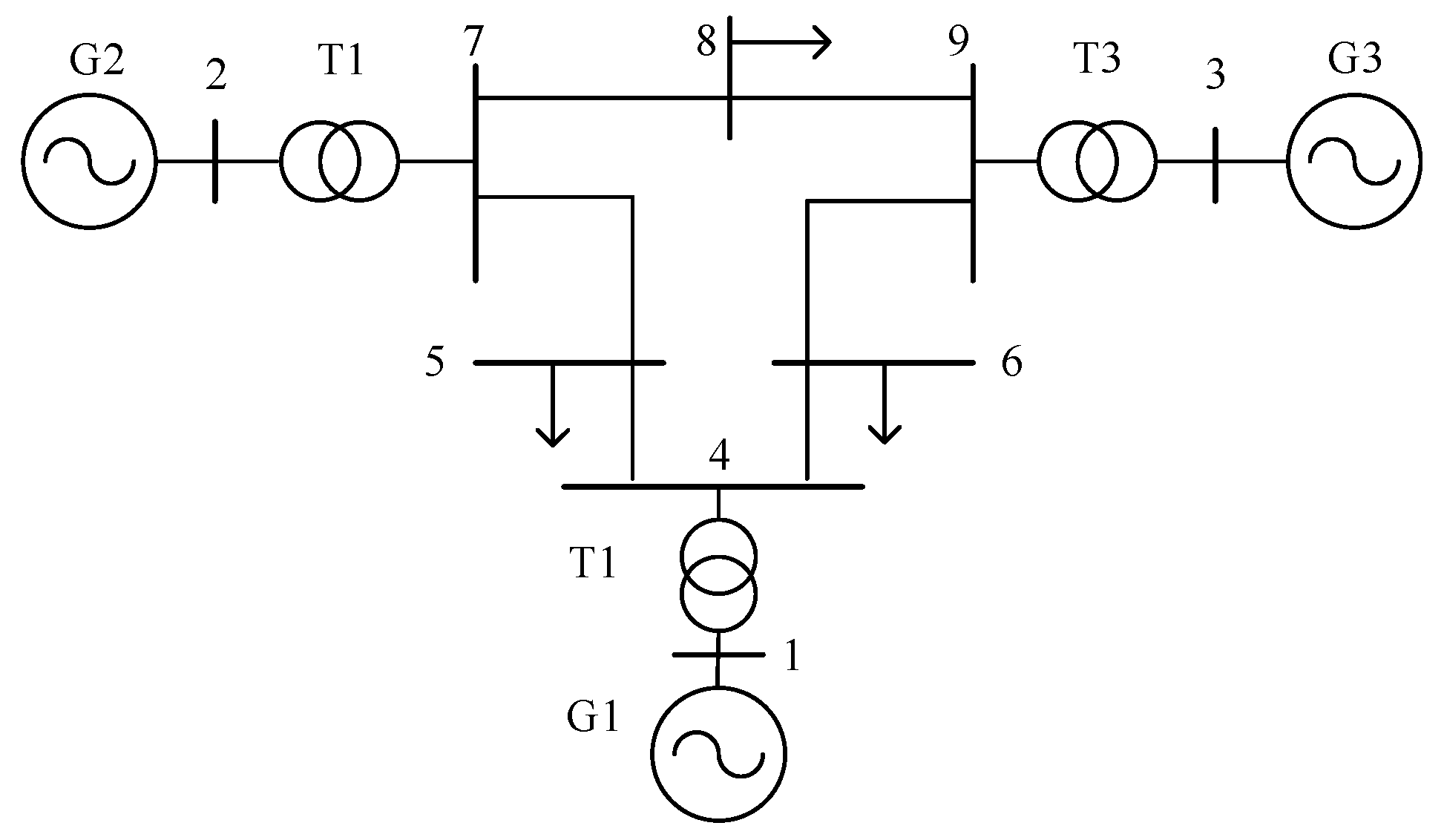
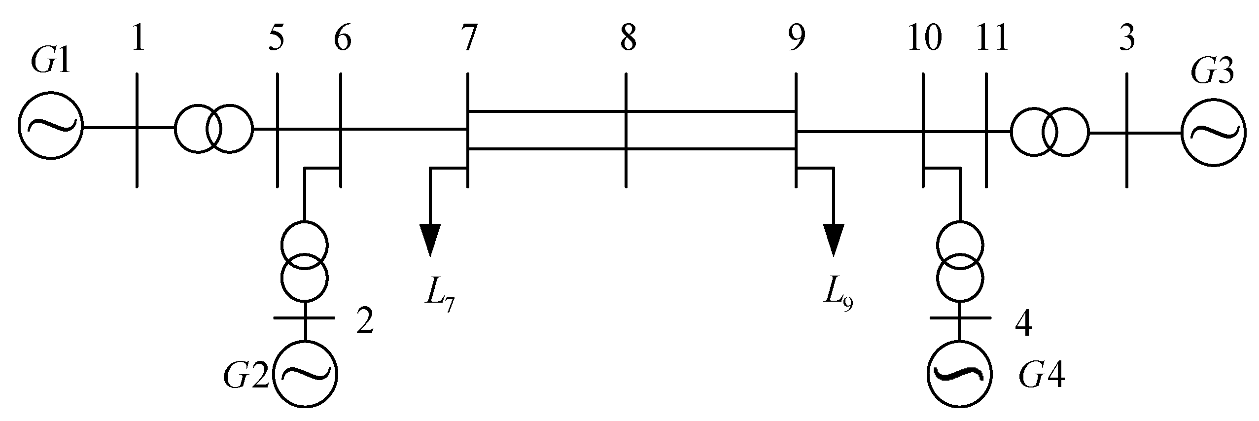
Consider an IEEE 3-machine 9-bus system with the system parameters as described in [28] and the topology as shown in Figure 6.
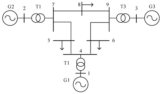
Figure 6.
3-machine and 9-bus system.
A 3-phase short-circuit fault is set to 0.2 s at bus 7, with the fault duration time set to 0.06 s. The rotor angle variations of the system described by Equations (22) and (30) are shown in Figure 7.
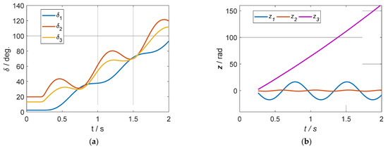
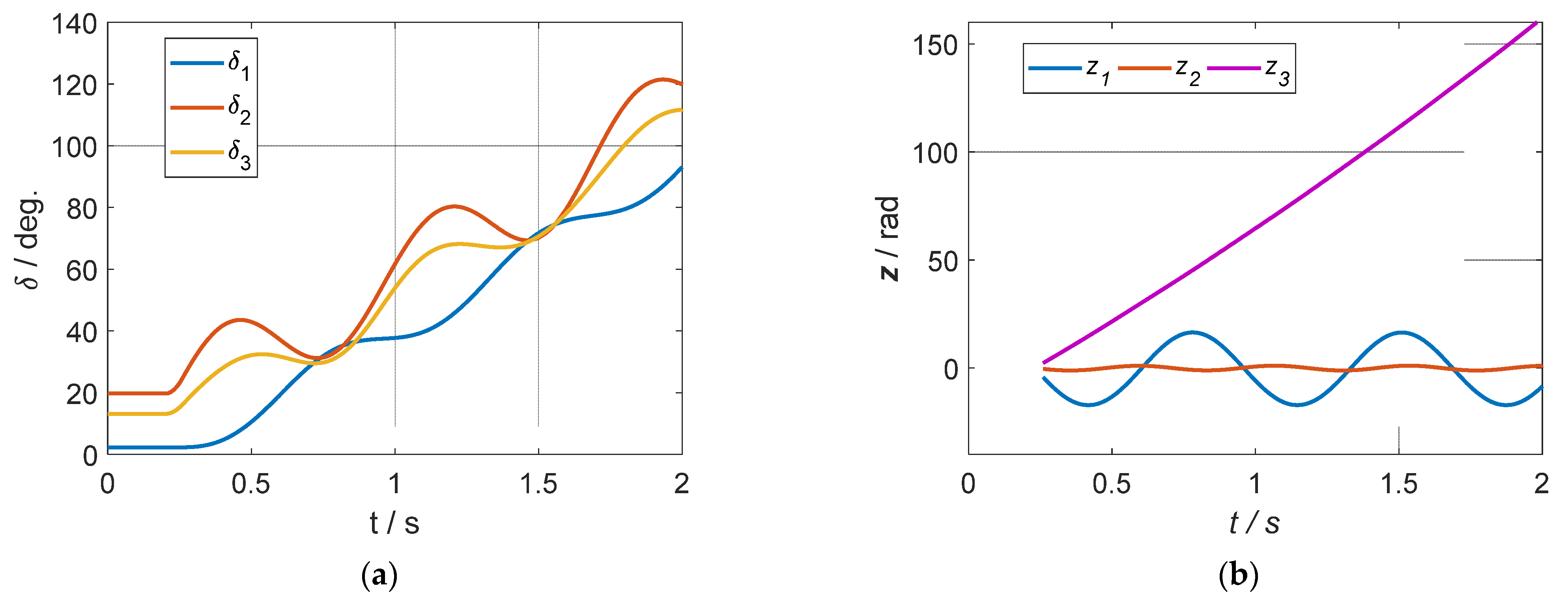
Figure 7.
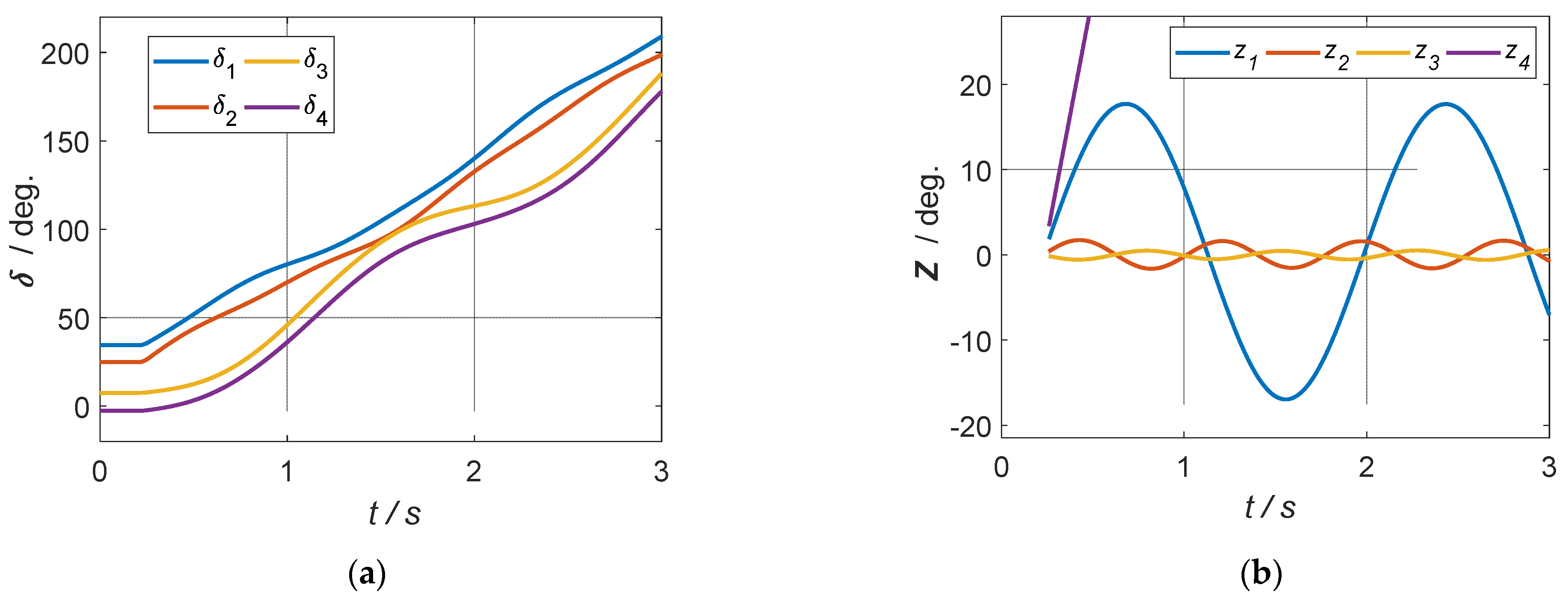
Response of rotor angle in different spaces. (a) The rotor angle response in the original space, i.e., δ coordinate system, governed by Equation (20); (b) the rotor angle response in Z space, i.e., Z coordinate system, governed by Equation (29).
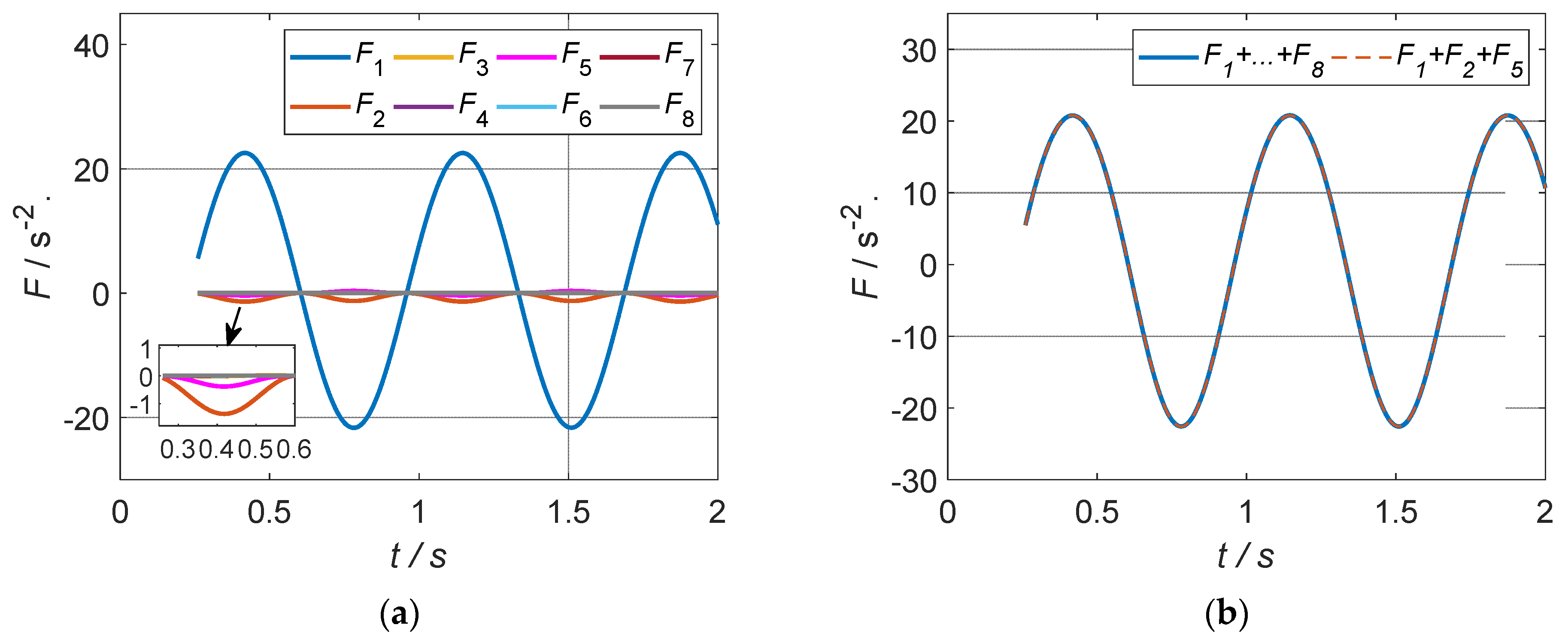
It can be observed that the rotor angle is moving forward after the clearance of fault in the δ coordinate system from Figure 7a. However, these motions can be divided into three parts, i.e., , , , where and are the oscillating components while is moving forward over time from Figure 7b, verifying the analysis from Equation (30). Moreover, the amplitude between and exhibits new characteristics, that is, , further validating the hypothesis in Section 3.3, that is, , where . Hence, the driving force governing the variation in can be divided as follows into eight parts according to Equation (35).
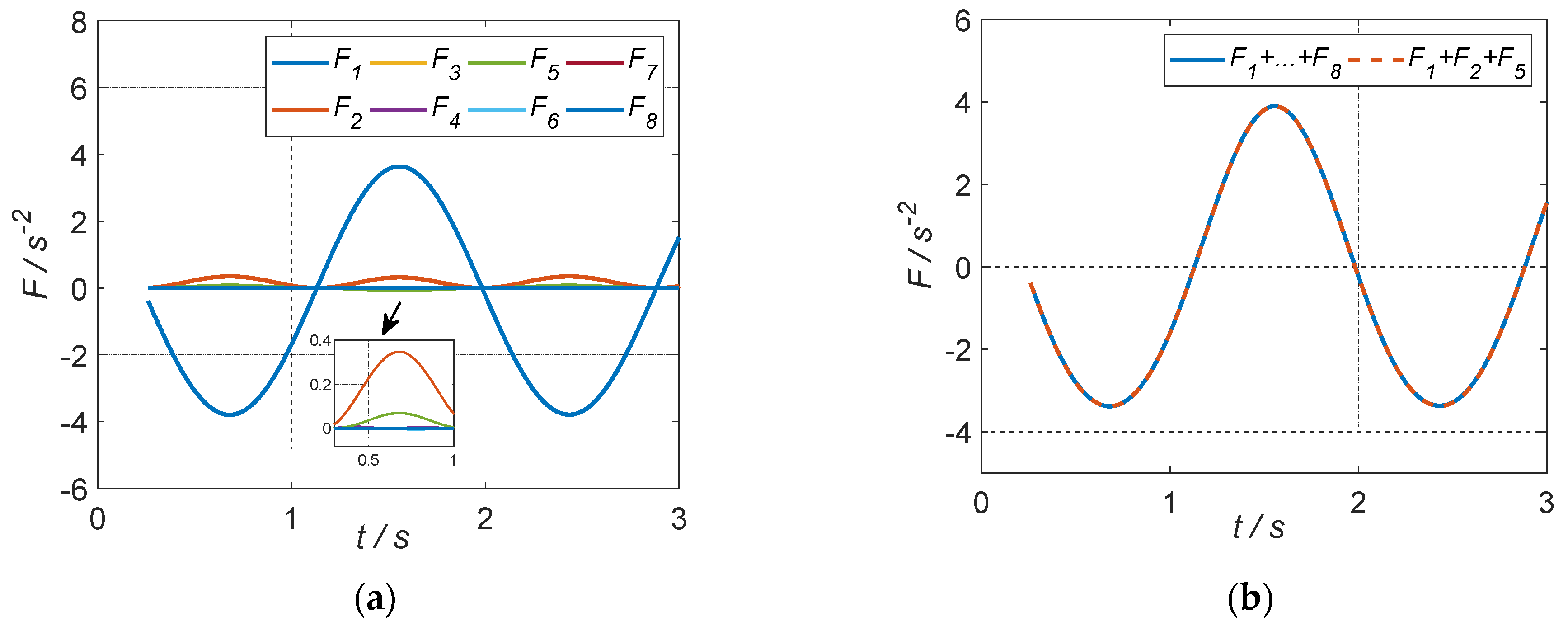
As shown in Figure 8a, among the nine types of forces driving the variations in , overwhelmingly dominate the other forces, and this fact can be observed from Figure 8b, which confirms the validity of Equation (36). Thus, the single-machine projection of the polynomial equation for a 3-machine 9-bus power system can be obtained as follows.
where . The V function implemented through the SOS method in Section 4 can proceed, and the value distribution of V function and its derivative is shown below.
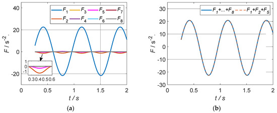
Figure 8.
Decomposition of the driving forces governing the variation in for IEEE 3-machine 9-bus system. (a) All the eight driving forces that dominate variation; (b) the three main driving forces that dominate variation.
The same observations can be made from Figure 9 as in the SMIB case, namely that the V function is positive in a large area near the origin (Figure 9a), while it is always negative near the origin for the derivative of the obtained V function (Figure 9b). This further confirms the fact that the V function obtained through the SOS method is a candidate function from Theorem 2. The domain of attraction of the single-machine system is plotted using this V function in Figure 10.
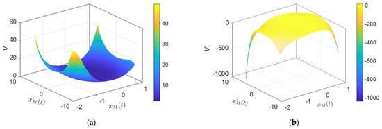
Figure 9.
Value distribution of V function and its derivative of a 3-machine 9-bus system. (a) Value distribution of the V function; (b) value distribution of the derivative of the V function.
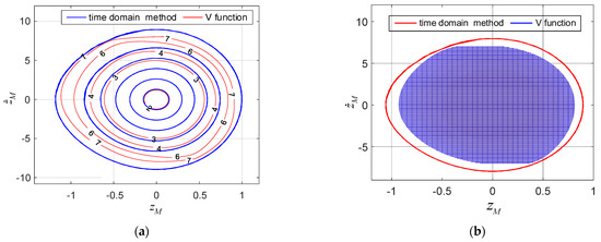
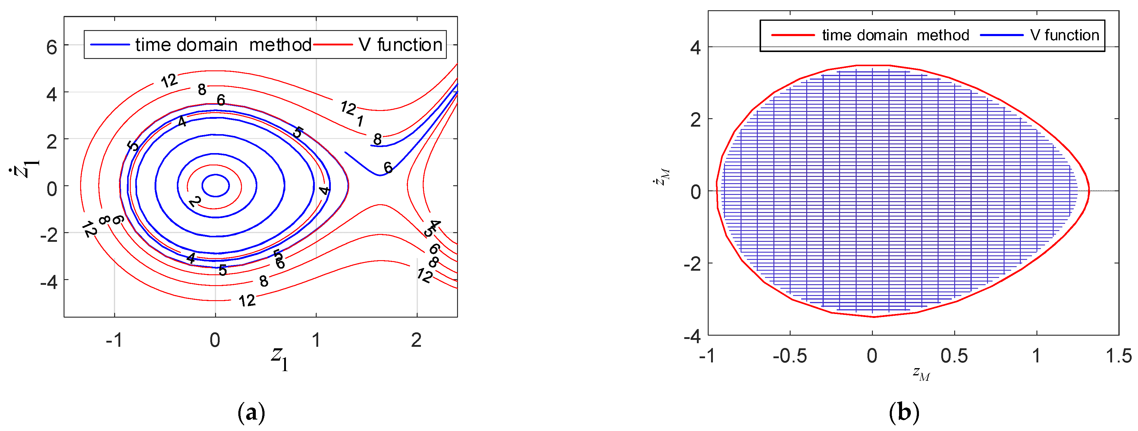
Figure 10.
Comparison diagram for the estimation of the domain of attraction of IEEE 3-machine 9-bus system. (a) Contour of the domain of attraction; (b) comparison with the time-domain method.
Compared to the time domain method, the estimation of the domain of attraction obtained through SOS is conservative, and this is due to the inherent numerical calculation characteristic of SOS when conducting the optimization procedure shown Figure 1. Once the optimization is claimed to have found a non-optimal solution, human intervention is also limited, resulting in the conservative property of the estimation of the region of attraction shown in Figure 10.
5.3. IEEE 4-Machine Test Power System
Consider an IEEE 4-machine 11-bus system with the system parameters as described in [29] and with the topology as shown in Figure 11.
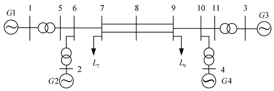
Figure 11.
4-machine and 11-bus system.
A 3-phase short-circuit fault is set to 0.2 s at bus 8, with the fault duration set to 0.06 s. The rotor angle variations described by Equation (22) and Equation (30), respectively, are shown in Figure 12.
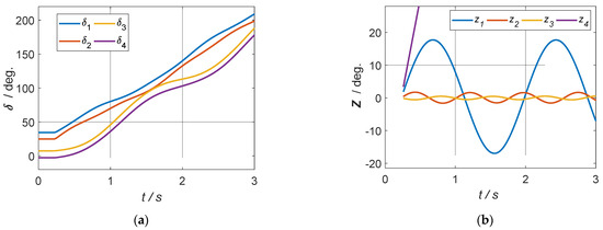
Figure 12.
Response of rotor angle in different spaces. (a) The rotor angle response in the original space, i.e., δ coordinate system, governed by Equation (20); (b) the rotor angle response in Z space, i.e., Z coordinate system, governed by Equation (29).
From Figure 12a, we can see that the rotor angle starts to rise at 0.02 s, indicating that the system dynamic process has begun. According to Equation (30), the angle dynamics in the original δ space can be transformed into the Z space shown in Figure 12b.
It can be observed from Figure 12b that the rotor angle dynamics in the original δ space can be decomposed into oscillating components, i.e., , and a linear component, i.e., , demonstrating the validity of the analysis in Section 3.2. Meanwhile, we can observe that and in Z space, manifesting the dynamic dominance of the variable. Additionally, the driving forces sustaining variation in can be decomposed into eight parts as follows.
We can see from Figure 13a that play a leading role among the driving forces, with these facts also observable in Figure 13b, showing that the summation of are almost equal to the right-hand side of Equation (35). Hence, the equation governing the variation in z1 can be rewritten as follows according to Equation (37).
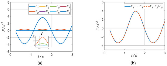
Figure 13.
Decomposition of the driving forces governing variation in for IEEE 4-machine 11-bus system. (a) All the eight driving forces that dominate variation; (b) the three main driving forces that dominate variation.
We can obtain the V function by applying the procedure in Figure 1, Section 4, based on Equation (51). The value distribution of the gained V function in three dimensions can be plotted as follows.
From Figure 14a,b, it can be observed that the V function is positive in a large area near the origin and the derivative of the obtained V function with time is negative, respectively. These facts show that the V function obtained through the SOS method satisfies the two conditions specified in Theorem 2, further verifying the validity of the V function. Moreover, the comparison of the domain of attraction between the V function and the time domain method is demonstrated as follows.
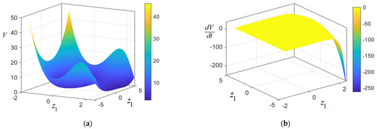
Figure 14.
Value distribution of the V function and its derivative of IEEE 4-machine 11-bus system. (a) Value distribution of the V function; (b) value distribution of the derivative of the V function.
It can be noticed that the domain of attraction determined by time domain method and the V function from Figure 15 exhibit a high degree of overlap, indicating that the proposed method can estimate the domain of attraction effectively. Furthermore, we define the set, , and the response of the system with different initial value is illustrated as follows.
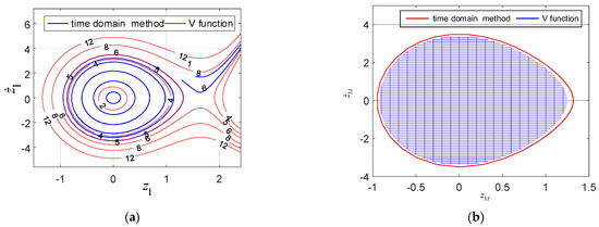
Figure 15.
Comparison diagram for the estimation of the domain of attraction of IEEE 4-machine 11-bus system. (a) Contour of the domain of attraction; (b) comparison with the time-domain method.
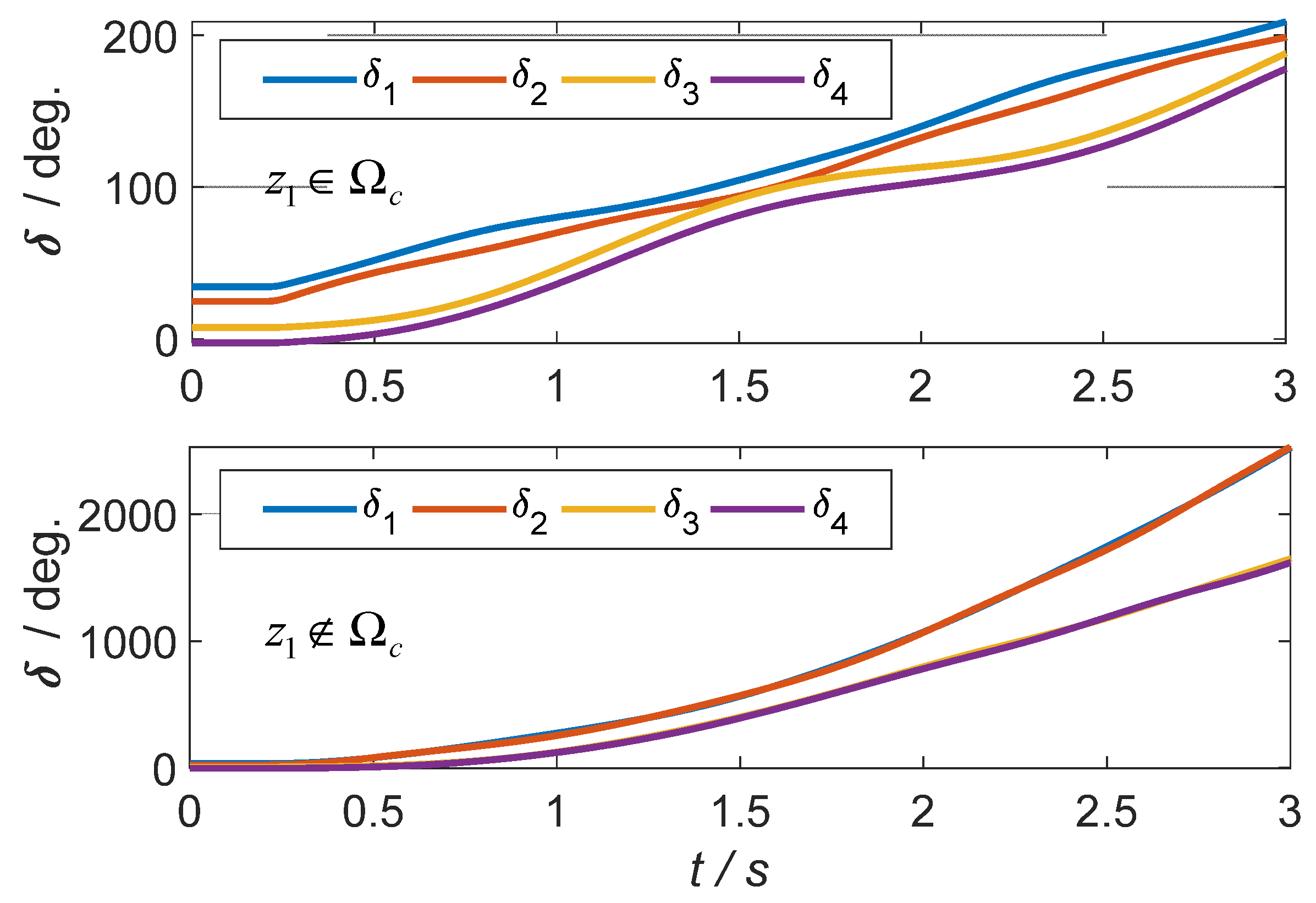
Figure 16 compares the system response following the input of different initial values. The result indicates that the system remains stable if the initial value is in the domain of attraction, i.e., , and vice versa. This shows that the estimated region of attraction can predict the qualitative behavior of the dynamic system, further verifying the effectiveness of the proposed method in estimating the region of attraction.
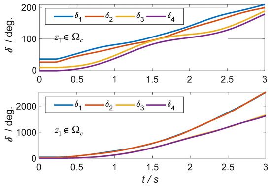
Figure 16.
Contour of the domain of attraction.
6. Conclusions
In this paper, leveraging the polynomial structural characteristics of power system swing equations, we propose an estimation method for the domain of attraction based on the SOS programming theory. The conclusions are as follows:
- (1)
- The swing equations of the power system exhibit inherent polynomial structural characteristics. Based on the Taylor expansion formula, the power system model in both single-machine and multi-machine scenarios can be unified in a polynomial framework.
- (2)
- Based on the amplitude characteristics of angles in Z space, a single-machine projection equation governing the variation of maximum angle for multi-machines power system is capable of determining the stability of the polynomial system.
- (3)
- Case studies of single-machine and multi-machine systems compared to the time-domain method demonstrate that the proposed method can compute the Lyapunov function (V function) and effectively estimate the domain of attraction of the power system.
This work contributes to the understanding of the polynomial structural characteristics of power systems and provides an estimation of the domain of attraction for polynomial-type power system equations using the SOS programming method. Further research should focus on accumulating experience in SOS programming and applying this differential algebra-based time domain method to various applications in power systems.
Author Contributions
Conceptualization, J.L.; formal analysis, H.W.; methodology, J.L. and X.Z.; project administration, D.G.; software, J.L. and H.W.; supervision, X.Z.; validation, J.L.; writing—original draft, J.L. and H.W.; writing—review & editing, X.Z. All authors have read and agreed to the published version of the manuscript.
Funding
This research was funded by the State Grid of China Corporation Headquarter Project “Renewable Power System Typical Instability Forms, Mechanisms and Analysis”, grant number 5108-202218280A-2-437-XG.
Data Availability Statement
The data presented in this study are available on request from the corresponding author. The data are not publicly available due to the first author’s PhD thesis having not been submitted at the time of publication of this work.
Acknowledgments
The main author (Jing Li) would like to thank the team (Hao Wu, Xianwen Zhan, and Deqiang Gan) for their continuous support and contributions toward this research and the College of Electrical Engineering at Zhejiang University for funding via a studentship bursary.
Conflicts of Interest
The authors declare no conflicts of interest.
References
- Khalil, H.K. Nonlinear Systems; Prentice Hall: Upper Saddle River, NJ, USA, 2002. [Google Scholar]
- Winfree, A.T. Biological rhythms and the behavior of populations of coupled oscillators. J. Theor. Biol. 1967, 16, 15–42. [Google Scholar] [CrossRef] [PubMed]
- Fouad, A.-A.; Vittal, V. Power System Transient Stability Analysis Using the Transient Energy Function Method; Pearson Education: Upper Saddle River, NJ, USA, 1991. [Google Scholar]
- Gassara, H.; Iben Ammar, I.; Ben Makhlouf, A.; Mchiri, L.; Rhaima, M. Design of Polynomial Observer-Based Control of Fractional-Order Power Systems. Mathematics 2023, 11, 4450. [Google Scholar] [CrossRef]
- Shakerighadi, B.; Ebrahimzadeh, E.; Blaabjerg, F.; Leth Bak, C. Large-signal stability modeling for the grid-connected VSC based on the Lyapunov method. Energies 2018, 11, 2533. [Google Scholar] [CrossRef]
- Parrilo, P.A. Structured Semidefinite Programs and Semialgebraic Geometry Methods in Robustness and Optimization; California Institute of Technology: Pasadena, CA, USA, 2000. [Google Scholar]
- Jarvis-Wloszek, Z.W. Lyapunov Based Analysis and Controller Synthesis for Polynomial Systems Using Sum-of-Squares Optimization; University of California, Berkeley: Berkeley, CA, USA, 2003. [Google Scholar]
- Tan, W. Nonlinear Control Analysis and Synthesis Using Sum-of-Squares Programming; ProQuest: Ann Arbor, MI, USA, 2006. [Google Scholar]
- Blekherman, G.; Parrilo, P.A.; Thomas, R.R. Semidefinite Optimization and Convex Algebraic Geometry; SIAM: Philadelphia, PA, USA, 2012. [Google Scholar]
- Tan, W.; Packard, A. Searching for control Lyapunov functions using sums of squares programming. In Proceedings of the 42nd Annual Allerton Conference on Communications, Control and Computing, Monticello, IL, USA, 29 September–1 October 2004; 2004; pp. 210–219. [Google Scholar]
- Papachristodoulou, A.; Prajna, S. A tutorial on sum of squares techniques for systems analysis. In Proceedings of the 2005, American Control Conference, Portland, OR, USA, 8–10 June 2005; pp. 2686–2700. [Google Scholar]
- Topcu, U.; Packard, A.; Seiler, P. Local stability analysis using simulations and sum-of-squares programming. Automatica 2008, 44, 2669–2675. [Google Scholar] [CrossRef]
- Khodadadi, L.; Samadi, B.; Khaloozadeh, H. Estimation of region of attraction for polynomial nonlinear systems: A numerical method. ISA Trans. 2014, 53, 25–32. [Google Scholar] [CrossRef] [PubMed]
- Ahmadi, A.A.; Majumdar, A. DSOS and SDSOS optimization: More tractable alternatives to sum of squares and semidefinite optimization. SIAM J. Appl. Algebra Geom. 2019, 3, 193–230. [Google Scholar] [CrossRef]
- Tacchi, M.; Cardozo, C.; Henrion, D.; Lasserre, J.B. Approximating regions of attraction of a sparse polynomial differential system. IFAC-PapersOnLine 2020, 53, 3266–3271. [Google Scholar] [CrossRef]
- Ameen, F.; Siddiq, A.; Trohák, A.; Benotsmane, R. A Scalable Hierarchical Dynamic PV Array Reconfiguration under Partial Shading. Energies 2024, 17, 181. [Google Scholar] [CrossRef]
- Anghel, M.; Milano, F.; Papachristodoulou, A. Algorithmic construction of Lyapunov functions for power system stability analysis. IEEE Trans. Circuits Syst. I Regul. Pap. 2013, 60, 2533–2546. [Google Scholar] [CrossRef]
- Mazumder, S.K.; de la Fuente, E.P. Dynamic stability analysis of power network. In Proceedings of the 2015 IEEE Energy Conversion Congress and Exposition (ECCE), Montreal, QC, Canada, 20–24 September 2015; pp. 5808–5815. [Google Scholar]
- Kundu, S.; Anghel, M. Stability and control of power systems using vector Lyapunov functions and sum-of-squares methods. In Proceedings of the 2015 European Control Conference (ECC), Linz, Austria, 15–17 July 2015; pp. 253–259. [Google Scholar]
- Han, D.; El-Guindy, A.; Althoff, M. Power systems transient stability analysis via optimal rational Lyapunov functions. In Proceedings of the 2016 IEEE Power and Energy Society General Meeting (PESGM), Boston, MA, USA, 17–21 July 2016; pp. 1–5. [Google Scholar]
- Mishra, C.; Thorp, J.S.; Centeno, V.A.; Pal, A. Stability region estimation under low voltage ride through constraints using sum of squares. In Proceedings of the 2017 North American Power Symposium (NAPS), Morgantown, WV, USA, 17–19 September 2017; pp. 1–6. [Google Scholar]
- Mishra, C.; Pal, A.; Thorp, J.S.; Centeno, V.A. Transient stability assessment of prone-to-trip renewable generation rich power systems using lyapunov’s direct method. IEEE Trans. Sustain. Energy 2019, 10, 1523–1533. [Google Scholar] [CrossRef]
- Izumi, S.; Somekawa, H.; Xin, X.; Yamasaki, T. Analysis of robust transient stability of power systems using sum of squares programming. Int. J. Electr. Power Energy Syst. 2020, 115, 105401. [Google Scholar] [CrossRef]
- Zhang, Z.; Schuerhuber, R.; Fickert, L.; Friedl, K.; Chen, G.; Zhang, Y. Domain of attraction’s estimation for grid connected converters with phase-locked loop. IEEE Trans. Power Syst. 2021, 37, 1351–1362. [Google Scholar] [CrossRef]
- Zhang, Q.; Gan, D. A Gronwall Inequality Based Approach to Transient Stability Assessment for Power Grids. arXiv 2023, arXiv:2311.02231. [Google Scholar]
- Chiang, H.-D.; Wu, F.F.; Varaiya, P.P. A BCU method for direct analysis of power system transient stability. IEEE Trans. Power Syst. 1994, 9, 1194–1208. [Google Scholar] [CrossRef]
- Topcu, U.; Packard, A.; Seiler, P.; Balas, G. Help on sos [ask the experts]. IEEE Control Syst. Mag. 2010, 30, 18–23. [Google Scholar]
- Anderson, P.M.; Fouad, A.A. Power System Control and Stability; John Wiley & Sons: Hoboken, NJ, USA, 2008. [Google Scholar]
- Kundur, P. Power system stability. Power Syst. Stab. Control. 2007, 10, 7–11. [Google Scholar]


Disclaimer/Publisher’s Note: The statements, opinions and data contained in all publications are solely those of the individual author(s) and contributor(s) and not of MDPI and/or the editor(s). MDPI and/or the editor(s) disclaim responsibility for any injury to people or property resulting from any ideas, methods, instructions or products referred to in the content. |
© 2024 by the authors. Licensee MDPI, Basel, Switzerland. This article is an open access article distributed under the terms and conditions of the Creative Commons Attribution (CC BY) license (https://creativecommons.org/licenses/by/4.0/).