
Effect of Cross Nanowall Surface on the Onset Time of Explosive Boiling: A Molecular Dynamics Study


Abstract
:1. Introduction
2. Simulation Method and Details
2.1. Simulation Details
2.2. Model Development
2.2.1. Force Field and Parameters
2.2.2. Simulation Boxes
2.3. Computational Runs
2.4. Post-Processing Analysis
3. Result and Discussion
3.1. Model Validation
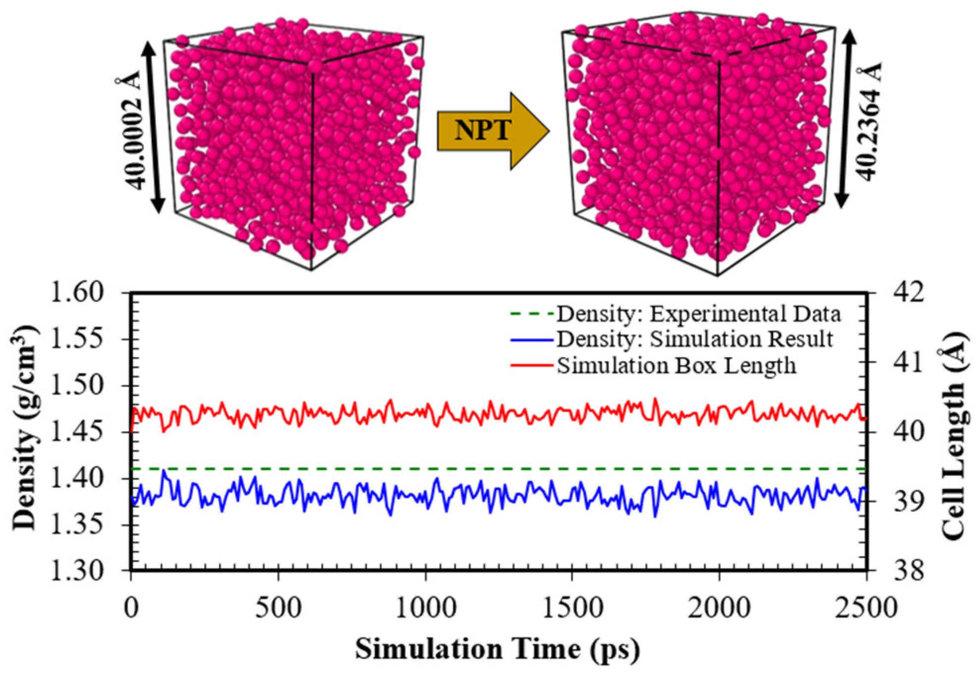
3.1.1. Simulation Case I: The Liquid Argon System
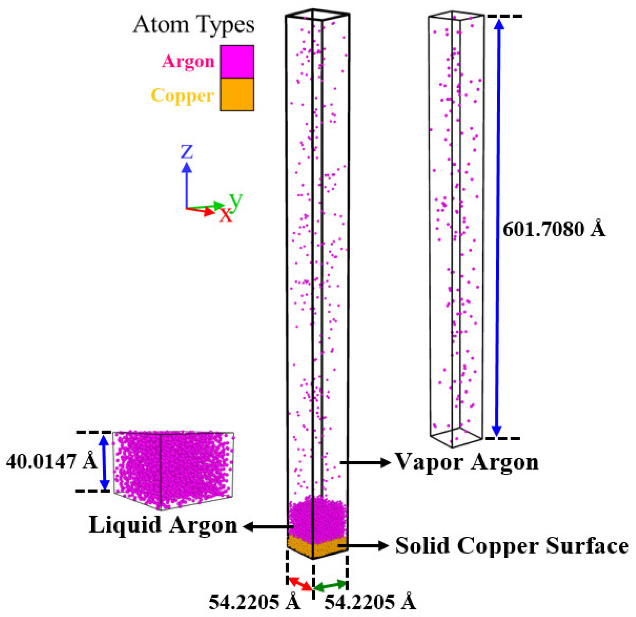
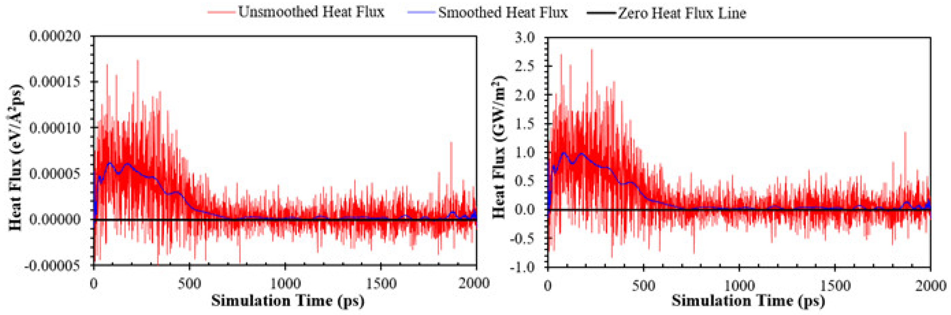
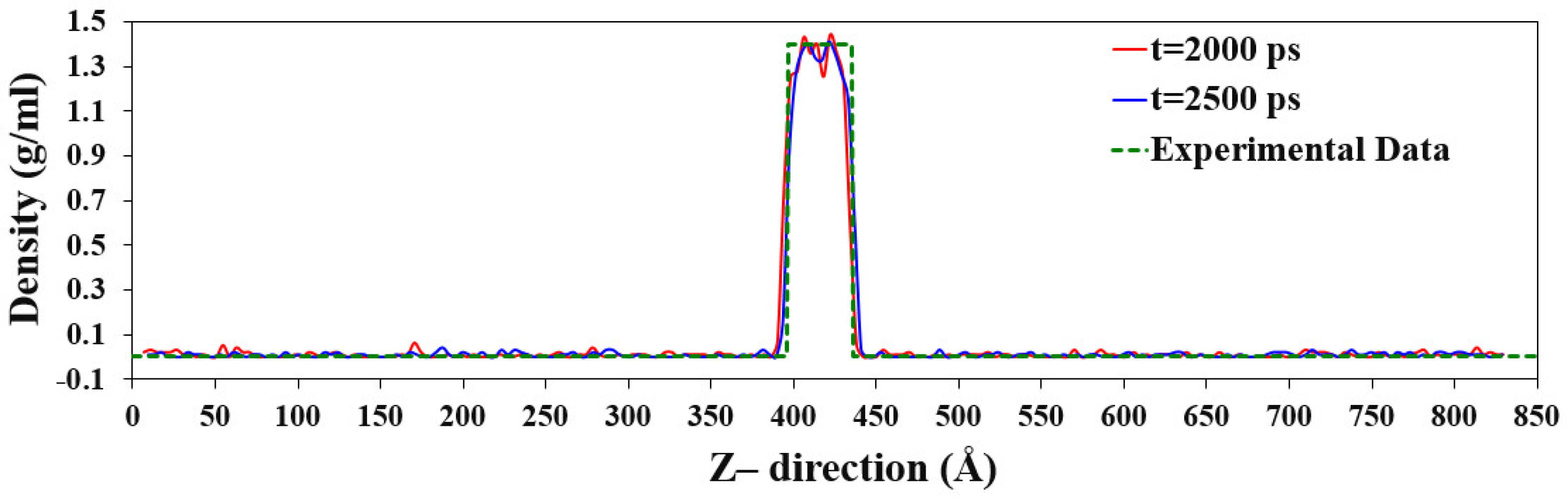
3.1.2. Simulation Case II: The Liquid–Vapor Argon Coexistence System
3.2. Simulation Cases A: Effects of Surface Topology and Spacing
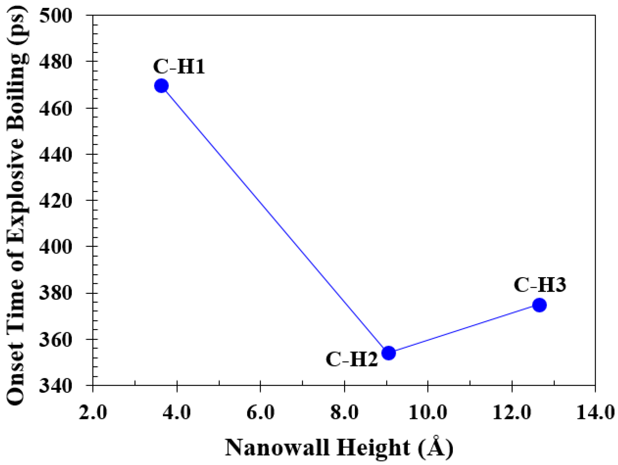
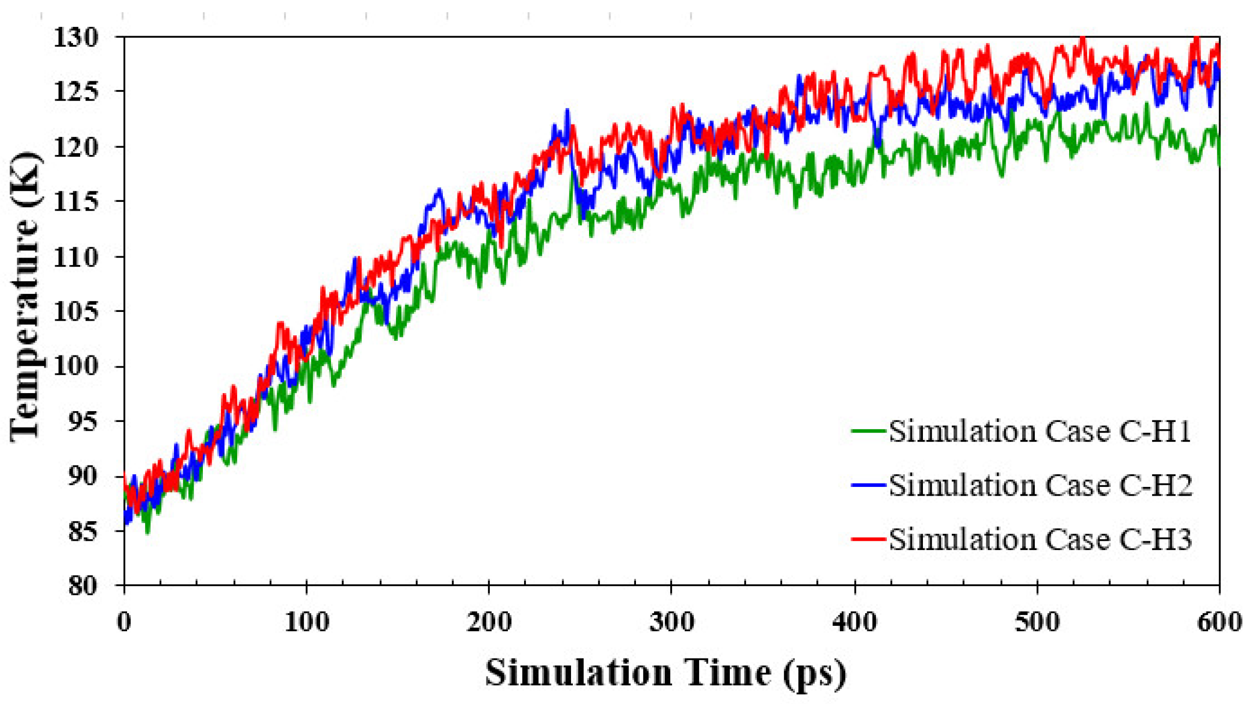
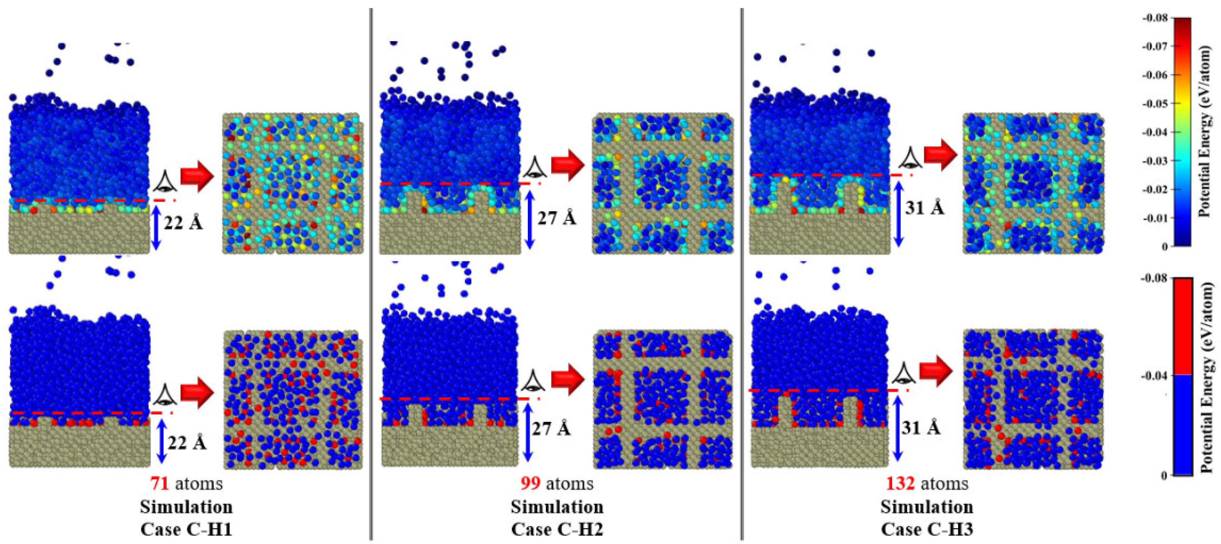
3.3. Simulation Cases B: Effects of Nanowall Height
4. Conclusions
- (1)
- The nanowalls make the interface area greater, allowing more heat to move from the solid to the liquid. This means that on the parallel and cross nanowall surfaces, explosive boiling happens faster than on the smooth surface.
- (2)
- The cross nanowalls, which have the same interface area as parallel ones, showed an earlier onset time for explosive boiling. This is because they provide greater movement space, so liquid argon atoms can escape more quickly from cross nanowalls than from parallel ones.
- (3)
- Decreasing the spaces between nanochannels decreases the onset time because it increases the interface area. But if we make the spaces even smaller than a certain point, it could slow down the movement of liquid atoms and postpone the explosive boiling.
- (4)
- Increasing the height of the nanowalls can decrease the onset time because it increases the interface area. However, if the nanowalls become too high, they can create a strong barrier, which takes longer to overcome and consequently postpones the onset time.
Supplementary Materials
Author Contributions
Funding
Data Availability Statement
Conflicts of Interest
Nomenclature
| A | Nominal surface area | (Å2) |
| Å | Angstrom | - |
| d | Lattice constant | (Å) |
| E | Young’s Modulus | (GPa) |
| Total energy of fluid atoms. | (eV) | |
| FCC | Face-centered-cubic | - |
| GW | Gigawatt | - |
| K | Spring constant | (eV/Å2) |
| L-J 12-6 | Lennard-Jones 12-6 | - |
| m | Meter | - |
| MDS | Molecular dynamics simulation | - |
| NVE | Microcanonical ensemble | - |
| NPT | Isothermal–isobaric ensemble | - |
| NVT | Canonical ensemble | - |
| OVITO | Open Visualization Tool | - |
| ps | Picosecond | - |
| q | Heat flux | (eV/Å2ps) |
| r | Distance between the particles | (Å) |
| RDF | Radial distribution function | - |
| t | Time | (ps) |
| T | Temperature | (K) |
| U | Potential energy | (eV) |
| Greek Symbols | ||
| Potential energy factor | - | |
| Energy parameter for L-J 12-6 potential | (eV) | |
| Length parameter for L-J 12-6 potential | (Å) | |
| Subscripts | ||
| Ar | Argon | |
| Cu | Copper | |
| i | Particle i | |
| j | Particle j | |
References
- Morshed, A.M.; Paul, T.C.; Khan, J.A. Effect of nanostructures on evaporation and explosive boiling of thin liquid films: A molecular dynamics study. Appl. Phys. A 2011, 105, 445–451. [Google Scholar] [CrossRef]
- Bai, P.; Zhou, L.; Du, X. Effects of surface temperature and wettability on explosive boiling of nanoscale water film over copper plate. Int. J. Heat Mass Transf. 2020, 162, 120375. [Google Scholar] [CrossRef]
- Mao, Y.; Zhang, Y. Molecular dynamics simulation on rapid boiling of water on a hot copper plate. Appl. Therm. Eng. 2014, 62, 607–612. [Google Scholar] [CrossRef]
- Ilic, M.; Stevanovic, V.D.; Milivojevic, S.; Petrovic, M.M. New insights into physics of explosive water boiling derived from molecular dynamics simulations. Int. J. Heat Mass Transf. 2021, 172, 121141. [Google Scholar] [CrossRef]
- Tang, Y.; He, Y.; Ma, L.; Zhang, X.; Xue, J. Molecular dynamics simulation of carbon nanotube-enhanced laser induced explosive boiling on a free surface of an ultrathin liquid film. Int. J. Heat Mass Transf. 2018, 127, 237–243. [Google Scholar] [CrossRef]
- Seyf, H.R.; Zhang, Y. Molecular dynamics simulation of normal and explosive boiling on nanostructured surface. ASME J. Heat Mass Transf. 2013, 135, 121503. [Google Scholar] [CrossRef]
- Kudryashov, S.I.; Allen, S.D. Photoacoustic study of explosive boiling of a 2-propanol layer of variable thickness on a KrF excimer laser-heated Si substrate. J. Appl. Phys. 2004, 95, 5820–5827. [Google Scholar] [CrossRef]
- Kudryashov, S.I.; Allen, S.D. Submicron dynamics of water explosive boiling and lift-off from laser-heated silicon surfaces. J. Appl. Phys. 2006, 100, 104908. [Google Scholar] [CrossRef]
- Seyf, H.R.; Zhang, Y. Effect of nanotextured array of conical features on explosive boiling over a flat substrate: A nonequilibrium molecular dynamics study. Int. J. Heat Mass Transf. 2013, 66, 613–624. [Google Scholar] [CrossRef]
- Wang, W.; Zhang, H.; Tian, C.; Meng, X. Numerical experiments on evaporation and explosive boiling of ultra-thin liquid argon film on aluminum nanostructure substrate. Nanoscale Res. Lett. 2015, 10, 158. [Google Scholar] [CrossRef]
- Fu, T.; Mao, Y.; Tang, Y.; Zhang, Y.; Yua, W. Effect of nanostructure on rapid boiling of water on a hot copper plate: A molecular dynamics study. Heat Mass Transf. 2016, 52, 1469–1478. [Google Scholar] [CrossRef]
- Zhang, S.; Hao, F.; Chen, H.; Yuan, W.; Tang, Y.; Chen, X. Molecular dynamics simulation on explosive boiling of liquid argon film on copper nanochannels. Appl. Therm. Eng. 2017, 113, 208–214. [Google Scholar] [CrossRef]
- Liu, H.; Qin, X.; Ahmad, S.; Tong, Q.; Zhao, J. Molecular dynamics study about the effects of random surface roughness on nanoscale boiling process. Int. J. Heat Mass Transf. 2019, 145, 118799. [Google Scholar] [CrossRef]
- Zhang, P.; Zhou, L.; Jin, L.; Zhao, H.; Du, X. Effect of nanostructures on rapid boiling of water films: A comparative study by molecular dynamics simulation. Appl. Phys. A 2019, 125, 142. [Google Scholar] [CrossRef]
- Liao, M.-J.; Duan, L.-Q. Explosive boiling of liquid argon films on flat and nanostructured surfaces. Numer. Heat Transf. Part A Appl. 2020, 78, 94–105. [Google Scholar] [CrossRef]
- Liu, H.; Deng, W.; Ding, P.; Zhao, J. Investigation of the effects of surface wettability and surface roughness on nanoscale boiling process using molecular dynamics simulation. Nucl. Eng. Des. 2021, 382, 111400. [Google Scholar] [CrossRef]
- Qasemian, A.; Qanbarian, M.; Arab, B. Molecular dynamics simulation on explosive boiling of thin liquid argon films on cone-shaped Al–Cu-based nanostructures. J. Therm. Anal. Calorim. 2021, 145, 269–278. [Google Scholar] [CrossRef]
- Zhou, J.; Li, S.; Tang, S.-Z.; Zhang, D.; Tian, H. Effect of nanostructure on explosive boiling of thin liquid water film on a hot copper surface: A molecular dynamics study. Mol. Simul. 2022, 48, 221–230. [Google Scholar] [CrossRef]
- Bai, P.; Zhou, L.; Du, X. Effects of liquid film thickness and surface roughness ratio on rapid boiling of water over copper plates. Int. Commun. Heat Mass Transf. 2021, 120, 105036. [Google Scholar] [CrossRef]
- Wang, R.; Qian, S.; Zhang, Z. Investigation of the aggregation morphology of nanoparticle on the thermal conductivity of nanofluid by molecular dynamics simulations. Int. J. Heat Mass Transf. 2018, 127, 1138–1146. [Google Scholar] [CrossRef]
- Yu, Y.; Xu, X.; Liu, J.; Liu, Y.; Cai, W.; Chen, J. The study of water wettability on solid surfaces by molecular dynamics simulation. Surf. Sci. 2021, 714, 121916. [Google Scholar] [CrossRef]
- Hu, C.; Shi, L.; Yi, C.; Bai, M.; Li, Y.; Tang, D. Mechanism of enhanced phase-change process on structured surface: Evolution of solid-liquid-gas interface. Int. J. Heat Mass Transf. 2023, 205, 123915. [Google Scholar] [CrossRef]
- Yin, X.; Hu, C.; Bai, M.; Lv, J. An investigation on the heat transfer characteristics of nanofluids in flow boiling by molecular dynamics simulations. Int. J. Heat Mass Transf. 2020, 162, 120338. [Google Scholar] [CrossRef]
- Leite, P.; de Koning, M. Nonequilibrium free-energy calculations of fluids using LAMMPS. Comput. Mater. Sci. 2019, 159, 316–326. [Google Scholar] [CrossRef]
- Stukowski, A. Visualization and analysis of atomistic simulation data with OVITO- the Open Visualization Tool. Model. Simul. Mater. Sci. Eng. 2010, 18, 015012. [Google Scholar] [CrossRef]
- Chen, Y.; Li, J.; Yu, B.; Sun, D.; Zou, Y.; Han, D. Nanoscale Study of Bubble Nucleation on a Cavity Substrate Using Molecular Dynamics Simulation. Langmuir 2018, 34, 14234–14248. [Google Scholar] [CrossRef]
- Zarringhalam, M.; Ahmadi-Danesh-Ashtiani, H.; Toghraie, D.; Fazaeli, R. Molecular dynamic simulation to study the effects of roughness elements with cone geometry on the boiling flow inside a microchannel. Int. J. Heat Mass Transf. 2019, 141, 1–8. [Google Scholar] [CrossRef]
- Delhommelle, J.; Millié, P. Molecular physics: An international journal at the interface between chemistry and physics. Mol. Phys. 2001, 99, 619–625. [Google Scholar] [CrossRef]
- Din, X.D.; Michaelides, E.E. Kinetic theory and molecular dynamics simulations of microscopic flows. Phys. Fluids 1997, 9, 3915–3925. [Google Scholar] [CrossRef]
- Hens, A.; Agarwal, R.; Biswas, G. Nanoscale study of boiling and evaporation in a liquid Ar film on a Pt heater using molecular dynamics simulation. Int. J. Heat Mass Transf. 2014, 71, 303–312. [Google Scholar] [CrossRef]
- Chen, Y.; Zou, Y.; Sun, D.; Wang, Y.; Yu, B. Molecular dynamics simulation of bubble nucleation on nanostructure surface. Int. J. Heat Mass Transf. 2018, 118, 1143–1151. [Google Scholar] [CrossRef]
- Reed, R.P.; Clark, A.F. Materials at low temperatures. Am. Soc. Met. 1983, 37, 8. [Google Scholar] [CrossRef]
- Hu, H.; Sun, Y. Effect of nanopatterns on Kapitza resistance at a water-gold interface during boiling: A molecular dynamics study. J. Appl. Phys. 2012, 112, 053508. [Google Scholar] [CrossRef]
- NIST Chemistry WebBook. NIST Standard Reference Database, NIST Chemistry WebBook. Available online: http://webbook.nist.gov/chemistry/ (accessed on 20 August 2023). [CrossRef]
- Hea, Y.; Wanga, S.; Tanga, Y.; Wub, Z.; Li, W. Molecular dynamics simulation on liquid nanofilm boiling over vibrating surface. Int. J. Heat Mass Transf. 2023, 201, 123617. [Google Scholar] [CrossRef]
- Deng, X.; Xu, X.; Song, X.; Li, Q.; Liu, C. Boiling heat transfer of CO2/lubricant on structured surfaces using molecular dynamics simulations. Appl. Therm. Eng. 2023, 219, 119682. [Google Scholar] [CrossRef]
- Wolde, P.R.T.; Frenkel, D. Computer simulation study of gas–liquid nucleation in a Lennard-Jones system. J. Chem. Phys. 1998, 109, 9901. [Google Scholar] [CrossRef]
- Wedekinda, J.; Reguera, D. What is the best definition of a liquid cluster at the molecular scale. J. Chem. Phys. 2007, 127, 154516. [Google Scholar] [CrossRef]
- Ilic, M.; Stevanovic, V.D.; Milivojevic, S.; Petrovic, M.M. Explosive boiling of water films based on molecular dynamics simulations: Effects of film thickness and substrate temperature. Appl. Therm. Eng. 2023, 220, 119749. [Google Scholar] [CrossRef]
- Yarnell, J.L.; Katz, M.J.; Wenzel, R.G.; Koenig, S.H. Structure factor and radial distribution function for liquid argon at 85 K. Phys. Rev. A 1973, 7, 2130–2144. [Google Scholar] [CrossRef]
- Liu, H.; Ahmad, S.; Chen, J.; Zhao, J. Molecular dynamics study of the nanoscale boiling heat transfer process on nanostructured surfaces. Int. J. Heat Mass Transf. 2022, 191, 122848. [Google Scholar] [CrossRef]
- Bai, P.; Zhou, L.; Du, X. Molecular dynamics simulation of the roles of roughness ratio and surface potential energy in explosive boiling. J. Mol. Liq. 2021, 335, 116169. [Google Scholar] [CrossRef]
- Alam, M.M.; Thakur, M.S.H.; Islam, M.; Hasan, M.N.; Mitsutake, Y.; Monde, M. Atomistic and macroscopic characterization of nanoscale thin film liquid-vapor phase change phenomena. Int. J. Therm. Sci. 2021, 170, 107159. [Google Scholar] [CrossRef]
- Wang, Y.-H.; Wang, S.-Y.; Lua, G.; Wang, X.-D. Explosive boiling of nano-liquid argon films on high temperature platinum walls: Effects of surface wettability and film thickness. Int. J. Therm. Sci. 2018, 132, 610–617. [Google Scholar] [CrossRef]
- Chen, Y.-J.; Lu, W.; Yua, B.; Tao, W.-Q.; Zhou, W.; Cao, Q. A revised Lennard-Jones potential for bubble nucleation study of argon based on the molecular dynamics simulation method. J. Mol. Liq. 2023, 371, 121094. [Google Scholar] [CrossRef]


 |  | 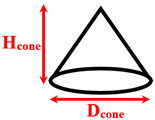 | |||
| Spherical nanopillar | Cylindrical nanopillar | Conical nanopillar | |||
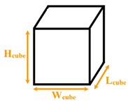 | 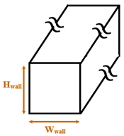 | ||||
| Cubical nanopillar | Cubical nanowall | ||||
| Study | Boiling Mode | Fluid/Solid Mediums | Nanostructure | Solid Surface Temperature (K) | |
| Topology (Shape) | Configuration (Size) * | ||||
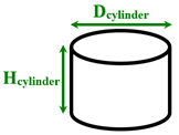
| Morshed et al. [1] | Normal/ Explosive | Argon/ Platinum | Separated cylindrical nanopillars | Dcylinder = 1.013 Hcylinder = 1.754–4.782 | 130 and 300 |
| Seyf and Zhang [6] | Normal/ Explosive | Argon/ Copper | Separated spherical nanopillars | Dsphere = 1–3 | 170 and 290 |
| Seyf and Zhang [9] | Explosive | Argon/ Aluminum and Silver | Separated conical nanopillars | Dcone = 1 Hcone = 2–5 | 270 |
| Wang et al. [10] | Normal/ Explosive | Argon/ Aluminum | Separated cubical nanopillars | Wcube = 1.8 Lcube = 1.8 Hcube = 1.8225–4.455 | 150 and 310 |
| Fu et al. [11] | Explosive | Water/ Copper | Separated cubical nanopillars | Wcube = 1.444–2.166 Lcube = 1.444–2.166 Hcube = 1.444–2.166 | 1000 |
| Zhang et al. [12] | Explosive | Argon/ Copper | Parallel cubical nanowalls | Wwall = 1.808 Hwall = 1.266–3.434 | 350 |
| Liu et al. [13] | Explosive | Argon/ Copper | Random roughness surface | – | 300 |
| Zhang et al. [14] | Explosive | Water/ Copper | Separated cubical nanopillars | Wcube = 1.444 Lcube = 1.444 Hcube = 1.444 | 800 |
| Liao and Duan [15] | Explosive | Argon/ Gold | Parallel cubical nanowalls | Wwall = 0.612 Hwall = 0.816–2.040 | 120–240 |
| Liu et al. [16] | Explosive | Argon/ Copper | Random roughness surface | – | 300 |
| Qasemian et al. [17] | Explosive | Argon/ Aluminum and Copper | Separated conical nanopillars | Dcone = 2.8 Hcone = 2 | 350 |
| Zhou et al. [18] | Explosive | Water/ Copper | Separated spherical and cylindrical nanopillars | Dsphere = 1–1.44 Dcylinder = 6 Hcylinder = 1.8 | 1000 |
| Atom Pairs | (Å) | (eV) |
|---|---|---|
| Cu-Cu | 1.9297 | 0.2047 |
| Ar-Ar | 3.4050 | 0.0104 |
| Ar-Cu | 2.6674 | 0.0065 |
 |  | 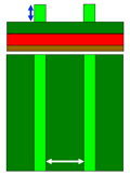 |  |
| Surface F | Surface P | Surface C | |
| The top and side schematic views of different copper surface topologies. | |||
| Simulation Case 1 | Spacing (Å) | Height (Å) | Surface Ratio 2 |
| 1. Simulation Cases A: different topologies with different spacing: | |||
| F | – | – | 1 |
| P-S1 | 50.6058 | 9.0368 | 1.3333 |
| P-S2 | 23.4956 | 1.6667 | |
| P-S3 | 14.4588 | 2.0000 | |
| P-S4 | 9.0368 | 2.3333 | |
| P-S5 | 7.2294 | 2.6667 | |
| P-S6 | 5.4220 | 3.0000 | |
| C-S1 | 50.6058 | 1.6444 | |
| C-S2 | 23.4956 | 2.2445 | |
| C-S3 | 14.4588 | 2.8000 | |
| C-S4 | 9.0368 | 3.3111 | |
| C-S5 | 7.2294 | 3.7778 | |
| F | – | 1 | |
| P-S1 | 50.6058 | 1.3333 | |
| 2. Simulation Cases B: cross nanowall surfaces with different heights: | |||
| C-H1 | 23.4956 | 3.6147 | 1.4978 |
| C-H2 | 9.0368 | 2.2445 | |
| C-H3 | 12.6515 | 2.7422 | |
Disclaimer/Publisher’s Note: The statements, opinions and data contained in all publications are solely those of the individual author(s) and contributor(s) and not of MDPI and/or the editor(s). MDPI and/or the editor(s) disclaim responsibility for any injury to people or property resulting from any ideas, methods, instructions or products referred to in the content. |
© 2024 by the authors. Licensee MDPI, Basel, Switzerland. This article is an open access article distributed under the terms and conditions of the Creative Commons Attribution (CC BY) license (https://creativecommons.org/licenses/by/4.0/).
Share and Cite
Fallahzadeh, R.; Bozzoli, F.; Cattani, L.; Azam, M.W. Effect of Cross Nanowall Surface on the Onset Time of Explosive Boiling: A Molecular Dynamics Study. Energies 2024, 17, 1107. https://doi.org/10.3390/en17051107
Fallahzadeh R, Bozzoli F, Cattani L, Azam MW. Effect of Cross Nanowall Surface on the Onset Time of Explosive Boiling: A Molecular Dynamics Study. Energies. 2024; 17(5):1107. https://doi.org/10.3390/en17051107
Chicago/Turabian StyleFallahzadeh, Rasoul, Fabio Bozzoli, Luca Cattani, and Muhammad Waheed Azam. 2024. "Effect of Cross Nanowall Surface on the Onset Time of Explosive Boiling: A Molecular Dynamics Study" Energies 17, no. 5: 1107. https://doi.org/10.3390/en17051107
APA StyleFallahzadeh, R., Bozzoli, F., Cattani, L., & Azam, M. W. (2024). Effect of Cross Nanowall Surface on the Onset Time of Explosive Boiling: A Molecular Dynamics Study. Energies, 17(5), 1107. https://doi.org/10.3390/en17051107