Article

Low-Voltage Distribution Network Loss-Reduction Method Based on Load-Timing Characteristics and Adjustment Capabilities

1
State Grid Jibei Electric Power Company Limited, Beijing 100054, China
2
Hubei Key Laboratory of Power Equipment & System Security for Integrated Energy, Wuhan 430072, China
3
School of Electrical Engineering and Automation, Wuhan University, Wuhan 430072, China
*
Author to whom correspondence should be addressed.
Energies 2024, 17(5), 1115; https://doi.org/10.3390/en17051115
Submission received: 28 January 2024 / Revised: 14 February 2024 / Accepted: 20 February 2024 / Published: 26 February 2024

Abstract

:
The primary contributors to elevated line losses in low-voltage distribution networks are three-phase load imbalances and variations in load peak–valley differentials. The conventional manual phase sequence adjustment fails to capitalize on the temporal characteristics of the load, and the proliferation of smart homes has opened up new scheduling possibilities for managing the load. Consequently, this paper introduces a loss-reduction method for low-voltage distribution networks that leverages load-timing characteristics and adjustment capabilities. This method combines dynamic and static methods to reduce energy consumption from different time scales. To commence, this paper introduced a hierarchical fuzzy C-means algorithm (H-FCM), taking into account the distance and similarity of load curves. Subsequently, a phase sequence adjustment method, grounded in load-timing characteristics, was developed. The typical user load curve, derived from the classification of user loads, serves as the foundation for constructing a long-term commutation model, therefore mitigating the impact of load fluctuations on artificial commutation. Following this, this paper addressed the interruptible and transferable characteristics of various smart homes. This paper proposed a multi-objective transferable load (TL) optimal timing task adjustment model and a peak-shaving control strategy specifically designed for maximum sustainable power reduction of temperature-controlled loads (TCL). These strategies aim to achieve real-time load adjustment, correct static commutation errors, and reduce peak-to-valley differences. Finally, a simulation verification model was established in MATLAB (R2022a). The results show that the proposed method mainly solves the problems of three-phase imbalance and large load peak–valley difference in low-voltage distribution networks and reduces the line loss of low-voltage distribution networks through manual commutation and load adjustment.

1. Introduction

The carbon dioxide emissions from the power sector constitute over 40% of the total carbon dioxide emissions in society [1]. Energy conservation and emission reduction in the electric power sector are pivotal for achieving dual carbon goals and will inevitably shoulder increased transformation responsibilities. Projections indicate that the share of new energy installed capacity is anticipated to approach 50% by 2030 and surpass 75% by 2060 [2]. This trajectory introduces heightened fluctuations in the system, necessitating enhanced flexible adjustment capabilities. The integration of a substantial proportion of distributed power sources holds the potential to not only reduce losses but also present challenges such as increased line losses, three-phase imbalance, and voltage deviation. These factors intensify the complexity of loss reduction in the distribution network [3]. Currently, primary loss-reduction measures on the distribution network side encompass network reconstruction [4], power flow optimization [5], three-phase imbalance control [6], and load peak shedding [7]. In low-voltage power distribution networks, the predominant methods typically employed are the latter two mentioned above.
Regarding the management of three-phase imbalance, the existing literature primarily addresses the constraints posed by three-phase loads in the operation of distribution networks. Literature [4] proposed a distribution network reconstruction method that considers the imbalance of three-phase load distribution to mitigate the impact of numerous distributed power sources and electric vehicles on three-phase imbalance. In a similar vein, Literature [8] investigates an optimal dispatch method under the coordination of Distributed Generation (DG) and Electric Vehicles (EV). It establishes a multi-objective optimization model that considers factors such as neutral line current, energy loss, voltage imbalance, and bus voltage, employing a differential evolution optimization algorithm for a solution. Another strategy focuses on transformer control, as seen in [9], which introduces a hybrid fuzzy controller-based control strategy to compensate for the neutral current generated by unbalanced renewable energy generation in low-voltage power grids while ensuring equal active power on both sides of the transformer. Additionally, efforts have been made to phase-convert single-phase loads for three-phase imbalance control. Literature [10] proposed an artificial commutation method that considers load–power transfer indicators to achieve three-phase imbalance control. Similarly, Literature [11] introduced a distribution network station phase sequence adjustment method, accounting for the timing characteristics and spatial distribution of single-phase source charge, to address three-phase imbalance at key nodes throughout the station area. While some studies manually switch user phase sequences, others explore the feasibility of automatic phase sequence switching. Literature [12] proposed a double-layer optimal phase switch device (PSD) layout model for mitigating three-phase imbalance. The upper-level goal is to minimize the total cost of PSD installation, and the lower-level goal is to minimize the operating cost on a typical day. Furthermore, the authors in [13] investigated the optimal number and installation locations of automatic phase commutation devices, considering reliability and economy. Manual commutation is deemed more economical since it does not require additional device installation. However, its real-time adjustment performance may not match that of automatic commutation devices. Considering the quadratic relationship between three-phase imbalance and line loss, manual phase commutation is deemed more economical for loss reduction.
The reduction of losses in low-voltage distribution networks can be approached not only through the balancing of three-phase loads but also by leveraging Home Energy Management Systems (HEMS) to optimize power usage patterns for peak shaving and valley filling [14]. In this context, the authors in [15,16] coordinate distributed photovoltaic and demand load resources based on user behavior predictions to formulate demand plans. Additionally, Literature [17] focuses on minimizing energy exchange with the power grid from the perspective of demand response. When smart homes actively participate in power grid operation and dispatch, ensuring user comfort is a crucial prerequisite [18]. Literature [19,20] introduces distinct smart home scheduling algorithms aiming to shift the use of electrical appliances from high electricity price periods to low electricity price periods, therefore reducing electricity bills and load peaks. The active involvement of smart homes in operation scheduling relies on the time-of-use electricity price strategy, prompting scholars to study optimal time-of-use electricity price strategies [21]. Furthermore, Literature [22,23] explores the formulation of optimal time-of-use electricity prices considering reliability loss and power loss, respectively. Smart homes can also passively and directly participate in operation scheduling through Internet of Things (IoT) technology. For instance, Literature [24] proposed a non-intrusive demand response approach, introduced advanced forecasting algorithms to predict HEMS occupancy using indirect data sources, and studied robust optimization strategies to deal with uncertainty. In another approach, Literature [25] considers the coordinated operation of micro-cogeneration and smart home appliances, proposing a day-ahead dispatch optimization model that incorporates demand response and wind power. The authors in [26,27], respectively, studied the deployment of HES and the reduction of residential energy consumption costs and proposed different algorithms to deal with comprehensive uncertainties. In general, by leveraging IoT technology, passive and direct participation in distribution network operation and dispatching can achieve more stable and reliable load peak shaving, therefore reducing network losses without compromising the user’s comfort level.
Presently, there is a notable gap in research concerning the integration of three-phase imbalance control and load peak shaving for loss reduction in low-voltage distribution networks. Furthermore, there is a lack of strategies addressing the simultaneous consideration of three-phase imbalance and real-time load dispatching operations. To fill this research gap, this paper proposes a loss-reduction method for low-voltage distribution networks based on load-timing characteristics and dispatching capabilities. Initially, considering the distance and similarity of load curves, this paper introduces a hierarchical fuzzy C-means algorithm (H-FCM) to classify user loads and form a typical user database. This forms the basis for establishing a long-term three-phase imbalance governance model. The Memetic Algorithm (MA) is employed to solve it, and the optimal access phase sequence for users is obtained. Static adjustment of the user phase sequence is then implemented to initially control three-phase imbalance and reduce network losses. Subsequently, acknowledging the interruptible and transferable characteristics of different smart homes, this paper presents a multi-objective transferable load (TL) optimal timing task adjustment model and a peak-shaving control strategy tailored for the maximum sustainable power reduction of temperature-controlled loads (TCL). For the TL timing adjustment model, the dynamically adjusted inertia weight improved particle swarm algorithm (IDWPSO) is utilized to solve the problem and obtain optimal timing instructions. While load peak shaving is executed, real-time control of three-phase imbalance is also considered, leading to a combined approach that further diminishes network losses. The overall program flow chart is depicted in Figure 1.
The innovation of this article lies in the following three points:
(1)
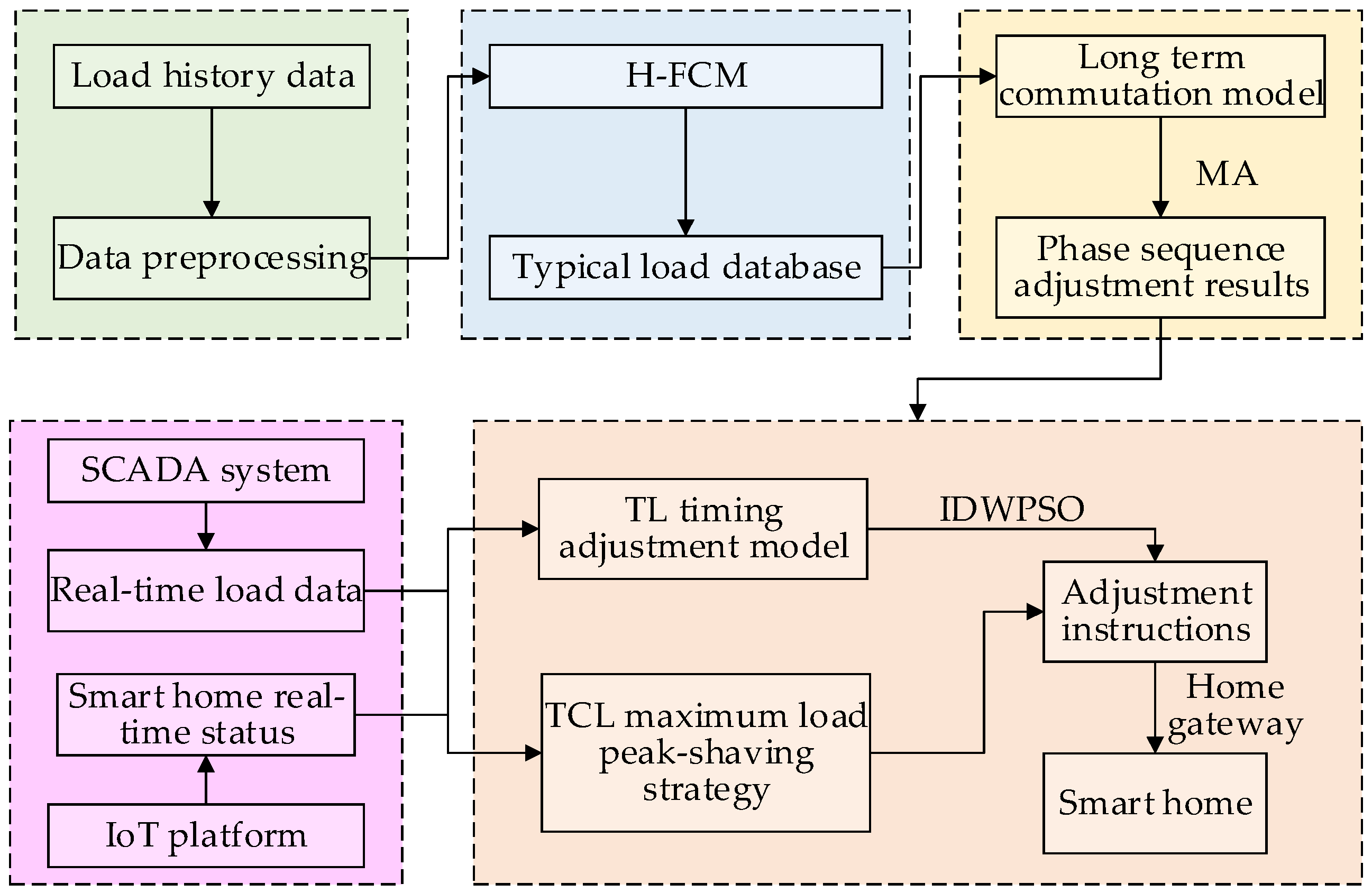
Addressing the distance and similarity of load curves, this paper introduces sequence variance to refine the clustering process. H-FCM is then proposed. The resulting typical load curve, formed after user classification, serves as the foundation for long-term commutation, mitigating the impact of load fluctuations on artificial commutation.
(2)
Recognizing the operational characteristics and adjustment methods of diverse smart homes, this paper presents a multi-objective TL optimal timing task adjustment model. Additionally, a peak-shaving control strategy is proposed to achieve the maximum sustainable power reduction for TCL.
(3)
The article focuses on controlling three-phase imbalance in low-voltage distribution networks from both static and real-time perspectives to enhance power quality. Simultaneously, load adjustment is employed to alter the shape of the load curve, reducing peak–valley differences and further minimizing line losses.

2. Demand-Side Resource Modeling Based on User Source Load Characteristics

2.1. Home Energy Management System Interaction Model

HEMS possesses the capability to comprehensively analyze information related to distributed power sources, loads, electricity prices, and more. Adjusting household loads enhances the electricity efficiency of residents, contributing to peak shaving, load leveling, and energy conservation [18]. The system architecture of HEMS, incorporating distributed photovoltaic power, is illustrated in Figure 2.
HEMS primarily governs the operation of smart home devices, each exhibiting unique operating characteristics that pose inherent challenges during adjustment and control. Based on the interruptability of power and the transferability of load sequences, smart homes are categorized into three groups: uncontrollable load (UL), transferable load, and temperature control load. Distinct control methods are employed for smart homes within each category. Table 1 provides an overview of typical smart home devices and their corresponding operating characteristics.
Currently, HEMS utilizes two main types of control methods for managing smart homes: electricity price incentives and centralized control. The electricity price incentive method relies on users’ proactive engagement, making it sensitive to electricity prices and resulting in relatively unstable adjustment effects. In contrast, centralized control involves directly managing the operational states of smart homes through the home gateway without compromising user comfort. This method proves more effective in household energy efficiency management compared to the electricity price incentive approach, and it finds widespread applicability in suitable contexts. The approach proposed in this article primarily focuses on centralized control as the research subject.

2.2. Modeling of Household Photovoltaic Panel Output Probability Characteristics

The majority of household photovoltaic panels are situated on the user’s roof, and their output is contingent on the lighting conditions and outdoor temperature. The light intensity is typically modeled using a Beta distribution [16], with its probability density function illustrated in Equation (1):
f ( S act ) = Γ ( a + b ) Γ ( a ) + Γ ( b ) S act S max a 1 1 S a c t S max b 1
where S a c t is the real-time light intensity, Γ is the Gamma function, S m a x is the maximum light intensity, a and b are the two shape parameters of the Beta distribution.
The output of household photovoltaic panels is directly proportional to the light intensity. The output at time t can be approximated by Equation (2):
P n , t PV = P PV S act S stc [ 1 + α PV ( T act T stc ) ]
where n is the user serial number, P n , t P V is the household photovoltaic panel output of user n at time t , P P V is the rated power of the household photovoltaic panel, S s t c is the rated light intensity of the household photovoltaic panel, α P V is the power temperature coefficient of the photovoltaic panel, T a c t is the actual temperature when the photovoltaic panel is in operation, T s t c is the rated temperature of the photovoltaic panel.

2.3. Load Resource Modeling Considering Scheduling Feasibility

2.3.1. Uncontrollable Load

Loads that remain beyond control during household load operation are termed uncontrollable loads. These loads cannot be interrupted, transferred in a time sequence, and possess a certain degree of volatility. The load fluctuation at each time point can be characterized by normal distribution [11], as illustrated in Equation (3):
f ( P n U L ) = 1 2 π σ exp ( P n U L μ ) 2 2 σ 2
where P n U L represents the size of the uncontrollable load for user n , σ is the standard deviation of the normal distribution, μ is the mean of the normal distribution.

2.3.2. Transferable Load

The transferable load exhibits characteristics of continuous operation, constant power, and a fixed working time. The operating period of this load type can be shifted, but it is constrained by the working time and the shiftable interval, as depicted in Equation (4):
Δ t max Δ t k Δ t max P k T L = c i r c s h i f t ( P k , 0 T L , Δ t k )
where k is the index of the TL device, Δ t k is the start and stop time offset of the timing task of TL device k , Δ t m a x is the start and stop time offset of the maximum timing task, P k T L is the power vector after the load translation of the TL device k , P k , 0 T L is the power vector before load translation of the TL device k , c i r c s h i f t ( ) is a cyclic translation array function, which translates the vector P k , 0 T L by Δ t k positions.

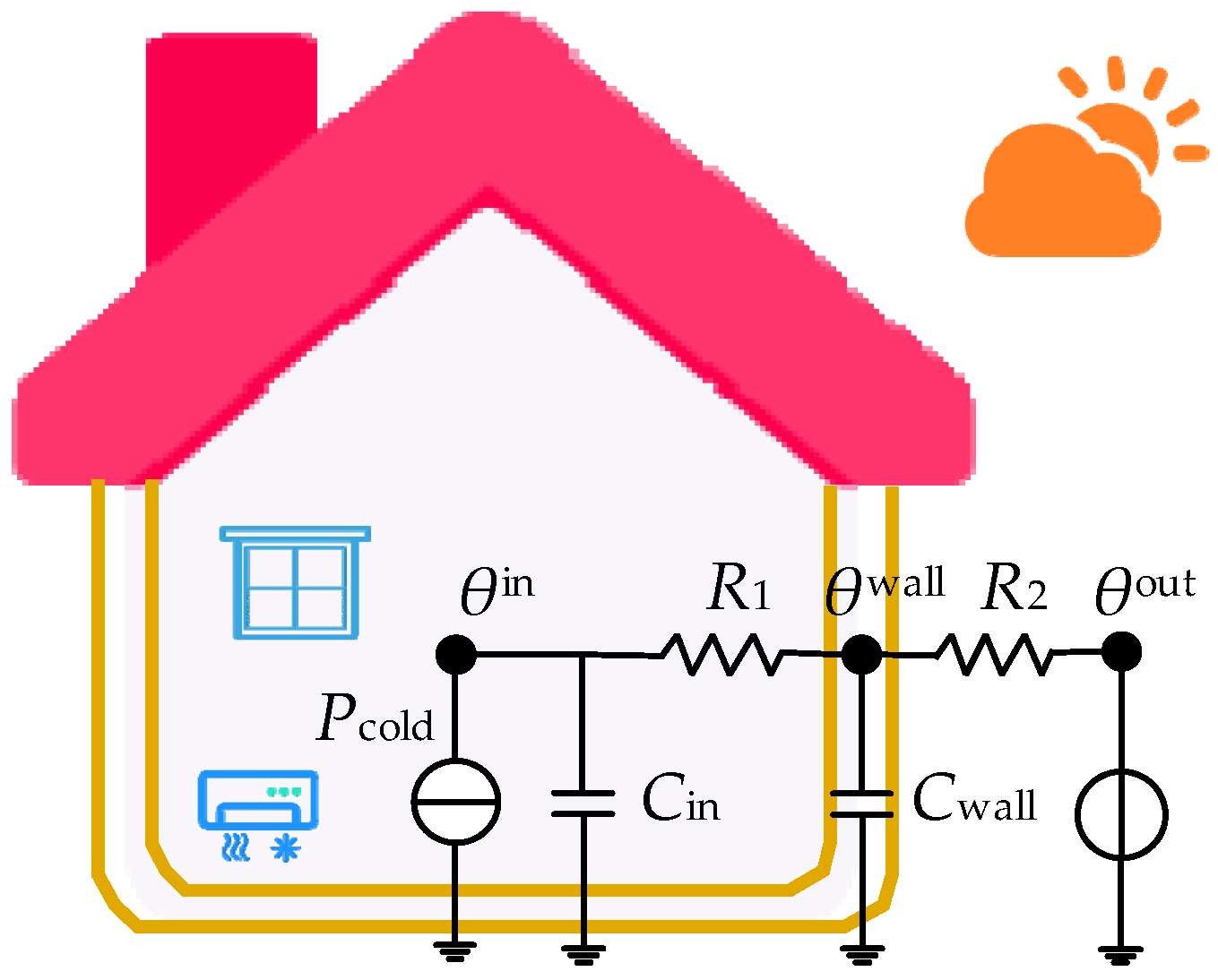
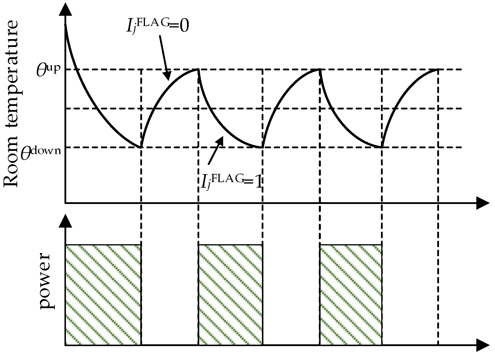
2.3.3. Temperature Control Load

The operating status of the temperature-controlled load is contingent on outdoor temperature, indoor temperature, temperature setting range, and the thermal parameters of the house. When the device is activated, the room temperature is expected to fall within the upper and lower limits of the set value. Air conditioning serves as a typical example of a temperature control load. The Equivalent Thermal Parameter (ETP) model is employed to elucidate the thermodynamic dynamic process of residential air conditioning, as illustrated in Figure 3.
According to Figure 3, the discretized ETP model describing the room temperature change process can be obtained, as shown in Equation (5).
θ in ( t + d t ) = θ in ( t ) + d t θ wall ( t ) θ in ( t ) R 1 P c o l d ( t ) C i n θ wall ( t + d t ) = θ wall ( t ) + d t θ out ( t ) θ wall ( t ) R 2 θ wall ( t ) θ in ( t ) R 1 C wall θ in ( 0 ) = θ in 0 , θ wall ( 0 ) = θ wall 0
where d t represents a discrete time period, and in this article, d t is set to 1 min.
When the TCL device is activated, its internal motor monitors variations in indoor temperature and dynamically adjusts the motor’s operational status based on whether it falls within the temperature control range. If the indoor temperature surpasses θ u p , the motor’s working status I j F L A G is set to 1, prompting a decrease in indoor temperature until it reaches the lower limit θ d o w n of the temperature control range. At this point, the motor’s working state I j F L A G is set to 0, allowing the indoor temperature to rise due to the influence of outdoor temperature. The motor’s working state will be reactivated the next time the indoor temperature reaches the upper limit of the temperature control range. The TCL device outputs power only when both the TCL device and its internal motor are operational, and the time interval of power output is influenced by the outdoor temperature and room parameters. The changes in room temperature during the air conditioner’s cooling state are illustrated in Figure 4.

3. Phase Sequence Adjustment Method Based on Load-Timing Characteristics

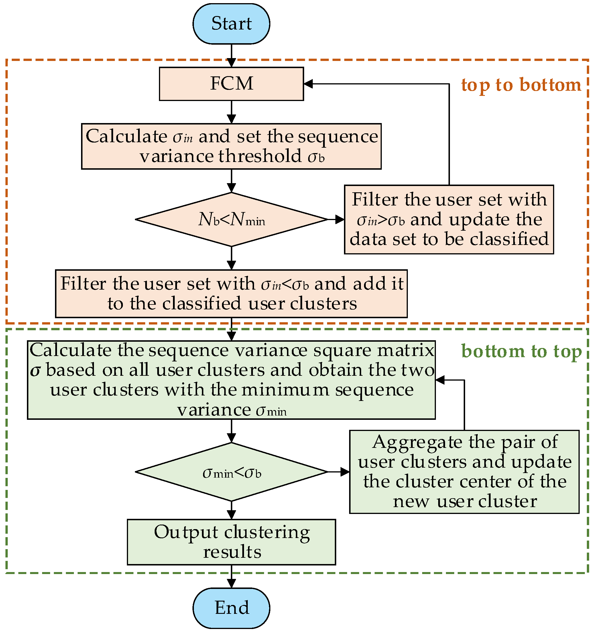
3.1. Load Classification Method Considering Distance and Similarity of Load Curves

There exist similarities and complementarities in the time series characteristics of residents’ load. By considering the load-timing characteristics shaped by users’ electricity consumption habits, it becomes possible to minimize overall three-phase imbalance through artificial phase modulation. The relationship between line loss and three-phase imbalance in a low-voltage distribution network approximately follows a quadratic function. In light of this, the reduction of line loss in the low-voltage distribution network necessitates manual adjustment of the user phase sequence to address the three-phase imbalance issue. This, in turn, requires precise load classification. To achieve this, the paper takes into account the distance and curve similarity of user historical load curves. It combines the concept of hierarchical clustering to merge similar data clusters and proposes H-FCM.
The fuzzy C-means algorithm (FCM) is an iterative clustering algorithm designed to assign individual data samples into multiple clusters. Assume that the typical daily historical load curve matrix P h of a low-voltage distribution network user is:
P h = [ P 1 h , P 2 h , , P n h , , P N h ]
where P n h is the typical daily historical load–power vector of user n , which is obtained by the weighted sum of the load curves of different typical days within a period of time; N is the total number of users.
Randomly select c rows of data from the P n h matrix as the initial clustering center matrix V 0 .The iterative formula for the membership matrix U and the cluster center matrix V are derived using the Lagrange multiplier method, as illustrated in Equations (7) and (8):
U i n v + 1 = l = 1 c ( d l n v + 1 ) 2 1 m 1 ( d i n v + 1 ) 2 1 m
V i v + 1 = n = 1 N ( U i n v ) m P n h n = 1 N ( U i n v ) m
where v is the number of iterations, i is the category subscript of the cluster center, U i n is the possibility that user n belongs to category i , c is the number of classifications in the data set, d i n is the Euclidean distance between i -th cluster center and user n data, representing the similarity between vectors, m is the fuzziness, with this article setting m = 2 , V i is the i -th clustering center vector.
When classifying users, the aforementioned FCM only takes into account the distance between data and does not consider the similarity of load curves. To address this, the paper introduces sequence variance to modify the clustering process. The calculation method for sequence variance is as shown in Equation (9):
σ i n = t = 1 T ( P n , t h V i , t ) mean ( P n h V i ) 2 T 1
where σ i n is the sequence variance of the typical daily load curve of type i -th cluster center and user n , T is the total number of sampling time points of typical daily load, t is the index of the sampling point, t ϵ [ 1 , T ] .
After introducing the sequence variance index, the conditions for sequence variance identification are established. Following multiple FCM user classifications, several sets of user clusters are obtained. Then, based on bottom-up hierarchical clustering, similar user clusters are merged to form new user clusters, ultimately resulting in a typical load database. Because there are numerous literature reports explaining FCM, this article focuses solely on detailing the proposed H-FCM. The process is illustrated in Figure 5.

3.2. Three-Phase Unbalanced Long-Term Commutation Model Based on Load–Power Consumption Characteristics

Utilizing the typical load database, the typical load of the user’s category serves as the foundation for adjusting the user’s phase sequence. By considering the average sharing within the same categories and mutual compensation between different categories, it becomes possible to reduce the three-phase imbalance of the distribution network through a single-phase sequence adjustment. This, in turn, leads to a reduction in the line loss of the distribution network.
The unreasonable load distribution between different phase sequences and the uncertainty of the load make the three-phase unbalanced phenomenon widely exist in the low-voltage distribution network [28]. Assume that the three-phase unbalanced distribution network has a total of c * type users after H-FCM clustering, and the number of type i users connected to phases A, B, and C are H A , i , H B , i , and H C , i , respectively. Then, the power vector P α h of each phase electric load at the low-voltage side gate of the distribution network transformer is:
P α h = i = 1 c H α , i × P i t
where α represents the three phases A, B, and C, P i t is the typical load–power vector of type i users.
Q/GDW 1519-2014 [29] “Regulations of operating and maintenance for distribution network” stipulates and quantifies the calculation method and balance degree of distribution transformer imbalance. The calculation of the three-phase imbalance is as follows:
g = max ( P α h ) min ( P α h ) max ( P α h )
where g is the instantaneous three-phase imbalance degree vector, m a x ( ) is the maximum value function, m i n ( ) is the minimum value function.
To consider the three-phase imbalance throughout the entire period during phase sequence adjustment, the objective is set to minimize the average three-phase imbalance throughout the day. Consequently, a phase sequence adjustment model for long-term control of three-phase imbalance was established, with the access phase sequence of each user as the optimization variable.
min α n g ¯ = t = 1 T g t T s . t . α n { A , B , C } H α , i = c o u n t ( α n = = α ) , n N i i = 1 c H A , i + H B , i + H C , i = N P α h = i = 1 c H α , i × P i t
where α n is the access phase sequence of user n ; g t is the instantaneous three-phase unevenness at time t ; N i is the sequence number set of type i users.
The MA is employed to solve the model. Previous literature has already validated the superiority of this algorithm in addressing similar problems [11]. The pseudo-code of the MA is provided in Appendix A.1.

4. Load Peak Shedding Method Considering Smart Home Adjustment Capabilities

4.1. Multi-Objective TL Optimal Timing Task Adjustment Model

TL achieves the purpose of smoothing load fluctuations and balancing three-phase loads by advancing or delaying the opening time. To ensure a positive user experience, the maximum movable time interval of TL needs to be defined, assuming it is [ Δ t m a x , Δ t m a x ] . Taking into account the sensitivity requirements of dynamic load adjustment, the status monitoring time scale of smart home device is set to 1 min. Through the SCADA monitoring system and the IoT cloud platform, real-time data of the distribution network and users can be obtained. The total load P α t o t a l of each phase, including household photovoltaic panels and different types of smart home loads, is calculated as follows:
P α total = α n = = α P n UL α n = = α P n PV + α k = = α P k TL + α j = = α P j , 0 TCL
where α k is the access phase sequence of TL device k ; α j is the access phase sequence of TCL device j ; P j , 0 T C L is the power vector of TCL device j .
Then, the instantaneous total load vector P t o t a l of the low-voltage distribution network is:
P total = α { A , B , C } P α total
The average three-phase imbalance based on real-time monitoring data of the distribution network is:
g ¯ = mean max ( P α total ) min ( P α total ) max ( P α total )
The coefficient of variation of the total load vector is utilized to measure the degree of load fluctuation. This is expressed as:
c v = n = 1 N P n total mean ( P total ) 2 / N mean ( P total )
Considering that the user experience is not affected as a constraint and the timing task movement time of the TL device is an optimization variable, a multi-objective TL optimal timing task adjustment model is established. The objective is to minimize three-phase imbalance and reduce load fluctuations.
min Δ t k β × g ¯ + ( 1 β ) × c v s . t . Δ t max Δ t k Δ t max P k TL = circshift ( P k , 0 T L , Δ t k )
where β is the optimization proportion coefficient of the average three-phase imbalance throughout the day, where β ϵ [ 0 , 1 ] .
For the above optimization model, the feasible space of decision variables is extensive, and there is a certain correlation between adjacent areas. Therefore, this paper utilizes IDWPSO to address the problem. With the introduction of the differential evolution operator, this algorithm exhibits higher solving efficiency and stronger global convergence compared to the traditional particle swarm algorithm. The pseudo-code of the IDWPSO is provided in Appendix A.2.

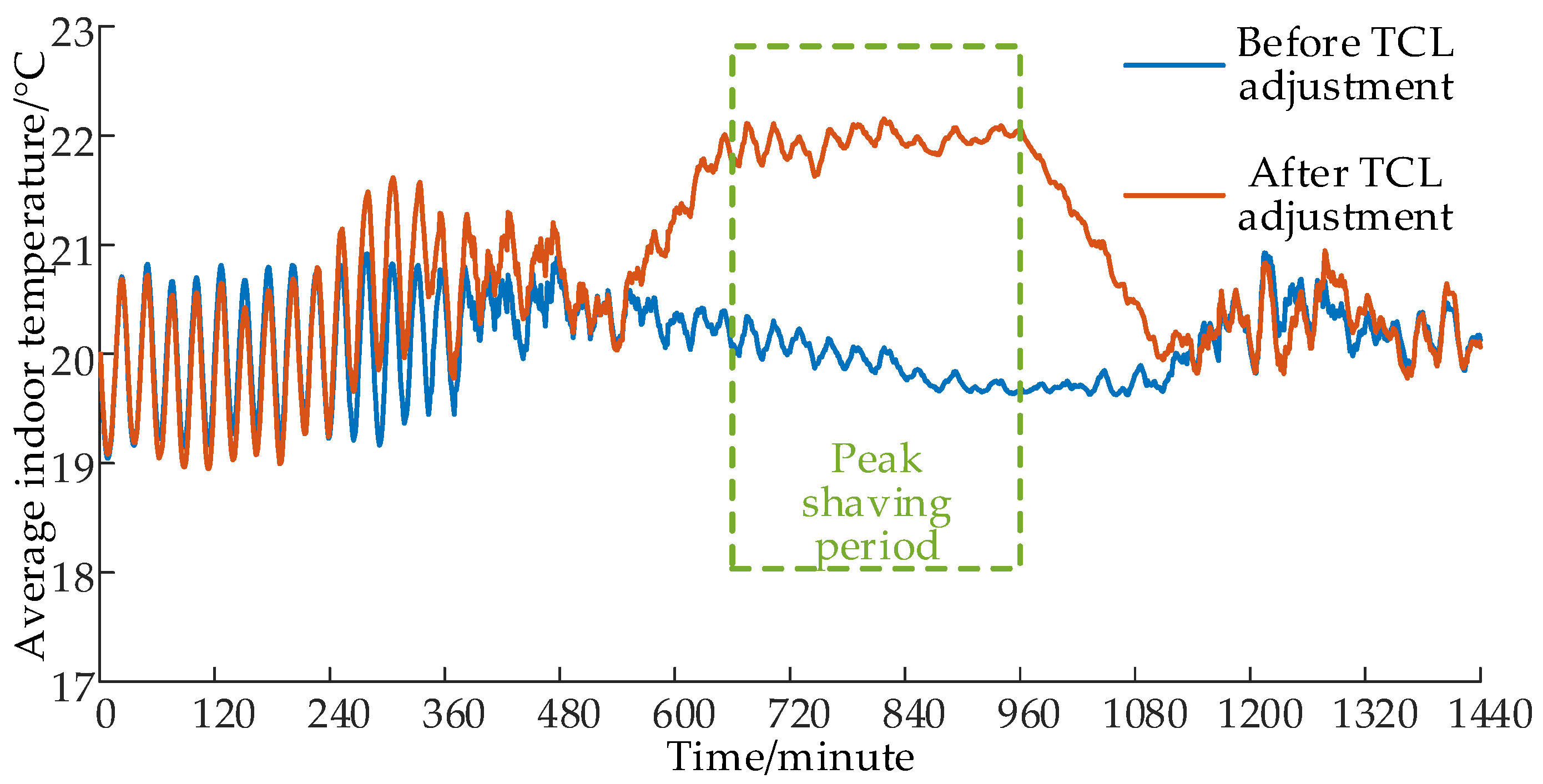
4.2. TCL’s Peak-Shaving Control Strategy for Maximum Sustainable Power Reduction Taking Comfort into Account

TCL can leverage the changing characteristics of indoor temperature to appropriately increase the indoor temperature during peak load periods, reducing the load without adversely affecting the user experience. This article proposes a peak-shaving control strategy based on the changes in the working status of the motor inside the TCL. The strategy is designed with four fundamental requirements: temperature control interval constraint, TCL device switching state constraint, maximum sustainable reduction power constraint, and three-phase imbalance constraint. The primary objective of this peak-shaving control strategy is to identify the instantaneous start–stop state changes in the motor inside the TCL while adhering to the specified constraints. The specific flow chart is illustrated in Figure 6 below.
(1)
Temperature control interval constraints. According to whether the indoor temperature θ j , t i n of the TCL device at time t is within the temperature control interval [ T d o w n , T u p ] , the working state vector of the motor inside the TCL device is determined as follows:
I j FLAG = 1 θ j , t in T up I j FLAG = 0 θ j , t in T down
(2)
TCL device switching state constraint. The working state vector I F L A G of the motor inside the TCL device is updated based on the switching state of the TCL device at time t + 1 , This is expressed as:
I j FLAG = 1 θ j , t in T up & I j , t + 1 status = = 1 I j FLAG = 0 others
where I j , t + 1 s t a t u s is the switching state of TCL device j at time t + 1 .
(3)
Maximum sustainable reduction power constraint. During the load peak shedding period, the number N 1 o f f of TCL internal motors that need to be shut down at time t + 1 is calculated based on the preset maximum sustainable reduction power P d o w n . The calculation formula is as follows:
N 1 off = ceil P down + sum ( I FLAG ) j = 1 J P j , 0 , t + 1 TCL P r TCL
where P j , 0 , t + 1 T C L is the power of TCL device j before regulation at time t + 1 ; P r T C L is the rated power of the TCL device.
Sort the indoor temperatures of the TCL internal motors from small to large according to the I F L A G obtained after constraining the switch status of the TCL device. Set the motor status corresponding to the first N 1 o f f TCL device to 0, and update I F L A G .
(4)
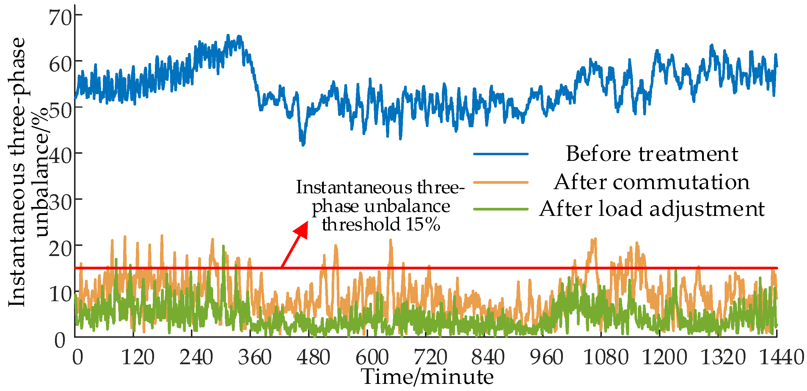
Three-phase imbalance constraint. Combined with the operating data of the low-voltage distribution network, calculate the instantaneous three-phase imbalance of the low-voltage distribution network at time t + 1 , the total power of each phase, the heavy-load phase and the light-load phase in the I F L A G working mode obtained after the previous update. According to Equations (21) and (22), the numbers N 2 o f f and N 2 o n of motors that need to be pre-closed and started are calculated:
N 2 off = round max ( P α total ) median ( P α total ) δ × P r TCL
N 2 on = round median ( P α total ) min ( P α total ) δ × P r TCL
where m e d i a n ( ) is the median function; δ is the three-phase imbalance constraint coefficient, which represents the constraints of the three-phase imbalance control strategy. The larger the value, the weaker the three-phase imbalance control effect, but the better the loss-reduction effect, δ ϵ [ 1 , + ] .
According to the I F L A G obtained in the previous step, sort the indoor temperatures at which the TCL internal motor is turned on from small to large. Set the motor status corresponding to the previous TCL device N 2 o f f to 0, and update I F L A G . Then, continue to sort the indoor temperatures from large to small for the TCL device with the internal motor turned off and the device status turned on. Set the motor status corresponding to the previous TCL device N 2 o n to 1, and update I F L A G . The final I F L A G obtained is passed to the TCL device through the home gateway as the TCL internal motor working state vector at time t + 1 to complete load regulation.

5. Simulation

5.1. Simulation Conditions

There are a total of 543 users in a low-voltage distribution network, including 3258 TL devices and 543 TCL devices. It is assumed that each household is equipped with a single-phase photovoltaic panel. The temperature on a typical day in summer is selected as the temperature reference. The sampling parameters of the TL and TCL device are shown in Table 2.
The equivalent model parameters of the temperature change process of a typical household (80 m2) are shown in Table 3.

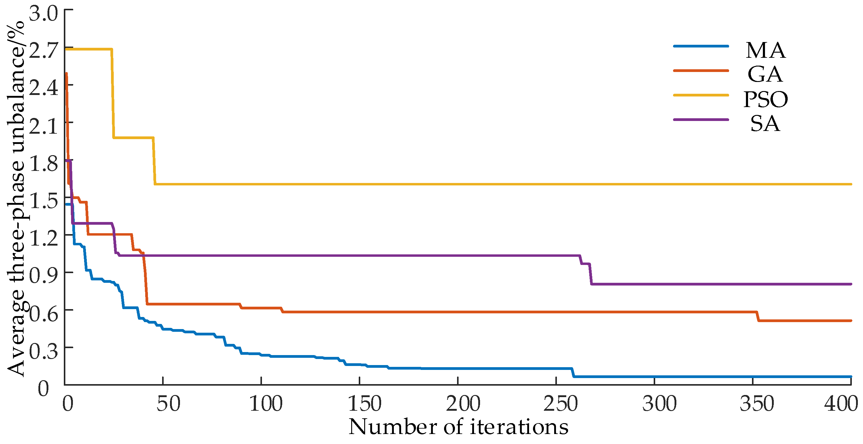
5.2. Phase Sequence Adjustment Results

The H-FCM algorithm proposed in this article is employed to cluster the typical daily load curves of distribution network users, resulting in the creation of a typical database, as illustrated in Figure 7.
The established typical load database is utilized, and the MA algorithm is applied to solve the long-term commutation model. Additionally, the performance of the genetic algorithm (GA), simulated annealing algorithm (SA), and particle swarm algorithm (PSO) in solving the model is compared. The initial total number of groups for various intelligent algorithms is set to 100, and the maximum number of iterations is 400 generations. The selection strategies for GA and MA are based on the roulette method, with a crossover probability of 0.8 and a mutation probability of 0.08. For SA, the initial temperature is set to 100, the temperature drop rate is 0.98, and the Metropolis criterion is used for the probability of accepting a differential solution. The algorithm evolution process when solving the long-term commutation model is depicted in Figure 8.
As observed in Figure 8, it is evident that the MA algorithm utilized in this study demonstrates superior convergence accuracy and speed compared to other intelligent optimization algorithms. However, since the long-term commutation model is based on static artificial phase modulation, it may not fully guarantee that the real-time average three-phase imbalance meets expectations. Therefore, subsequent adjustments of the load by smart homes are necessary to achieve the desired outcomes.

5.3. Loss-Reduction Effect

The real-time operation data of the distribution network and the status of smart homes, monitored by the IoT platform through SCADA, are acquired. These data are then input into the TL optimal timing task adjustment model, and the IDWPSO is employed to address the problem. Setting β = 0.8 is primarily aimed at minimizing real-time three-phase imbalance. The settings for the remaining intelligent optimization algorithms are consistent with the parameters mentioned earlier. The algorithm’s evolutionary process in solving the TL timing optimization model is illustrated in Figure 9.
Indeed, as depicted in Figure 9, IDWPSO exhibits commendable performance in solving the TL timing optimization model. The integration of differential evolution has proven effective in addressing issues related to population diversity reduction in later iterations of the particle swarm algorithm, mitigating the tendency to converge to local optimal solutions and enhancing the overall global search capability.
Regulation in accordance with the peak-clipping control strategy for TCL’s maximum sustainable power reduction resulted in instructions for controlling the TCL motors, as illustrated in Figure 10, which showcases a comparison of average temperatures before and after adjustment during TCL operation. Additionally, Figure 11 provides a histogram depicting the number of times the TCL motors participate in the regulation.
The comparison of instantaneous three-phase imbalance at different stages is depicted in Figure 12. The average three-phase imbalance before governance is 54.049%. After the phase sequence adjustment, the average three-phase imbalance decreases to 9.084%, with 162 time points exceeding the 15% limit. Following real-time treatment, the average three-phase imbalance further reduces to 4.468%, and there are only 10 time points exceeding the 15% limit. The improvement in the three-phase imbalance is evident.
The instantaneous power comparison at different stages is illustrated in Figure 13. The line loss rate before treatment was 5.044%, and after phase sequence adjustment, it decreased to 4.300%. Following load adjustment, the line loss rate further decreased to 3.949%, marking a reduction of 1.095 percentage points compared to the line loss rate before treatment. The comprehensive power loss before treatment was 1187.541 kWh, while after the phase sequence adjustment, it decreased to 1004.333 kWh. After load adjustment, the comprehensive power loss further decreased to 868.856 kWh, resulting in a total saving of 318.685 kWh compared to the entire day before treatment.

5.4. Loss-Reduction Effects in Different Scenarios

To further explore the impact of long-term commutation and smart home load adjustment, as well as the impact of different types of smart homes on loss reduction and three-phase imbalance control, this article set up different experimental groups to analyze and study this method. Set up the following four sets of comparison scenarios, and mark the simulation scenarios mentioned above as #S5.
#S1: No long-term commutation, only adjustment of smart home load.
#S2: Only long-term phase commutation is performed, and no smart home load adjustment is performed.
#S3: Perform long-term commutation while only adjusting the TL.
#S4: Perform long-term commutation while only adjusting the TCL.
Compare the following indicators of the treated low-voltage distribution network: average three-phase imbalance, peak-to-valley ratio, line loss rate, and line loss. The comparison results are shown in Table 4.
From the comparison results in the above table, it can be found that long-term commutation mainly reduces line losses by reducing the three-phase imbalance, and smart home load adjustment mainly reduces line losses by reducing the peak-to-valley ratio. The timing shift of TL mainly reduces the instantaneous three-phase imbalance, while TCL mainly reduces the peak-to-valley ratio. In general, the treatment method proposed in this article that combines long-term commutation and smart home load adjustment has the most obvious effect in reducing line losses.

6. Conclusions

(1)
The introduced H-FCM algorithm not only takes into account the distance of load curves but also considers the similarity of load curves. Through load classification, a typical load curve is derived, and a long-term commutation model is established and solved using the MA algorithm. This approach reduces the influence of load uncertainty on artificial commutation results, enhancing the robustness of the long-term commutation model.
(2)
Considering the output characteristics of TL, this paper proposes a multi-objective TL optimal timing task adjustment model solved by IDWPSO. Additionally, a peak-cutting control strategy for maximum sustainable power reduction is introduced based on the monitoring of indoor temperature, ensuring it does not impact the user experience. The effectiveness of this strategy is validated through simulations.
(3)
Our approach primarily addresses issues related to three-phase imbalance and significant load peak–valley differences in low-voltage distribution networks. By incorporating manual commutation and load adjustments, this paper successfully reduces line losses. Simulation results demonstrate a noteworthy electricity savings of 318.685 kWh throughout the day, accompanied by a reduction of 1.095 percentage points in the line loss rate. The overall impact on loss reduction is substantial.
The loss-reduction method presented in this paper considers two key factors influencing line losses: three-phase imbalance and load peak–valley differences. By combining dynamic and static approaches in terms of long-term commutation and real-time adjustments, the line losses in the low-voltage distribution network are effectively reduced. Simulation results demonstrate a substantial improvement in line losses after treatment, showcasing evident economic benefits. This approach offers valuable technical guidance for line loss management in similar scenarios. However, it is important to note that the method outlined here has high data requirements for regulating smart home devices. In the future, it is necessary to further classify and model smart homes, electric vehicles, and multiple energy storage loads, and more consideration will be given to the impact of user behavior and the interaction between different smart homes on modeling. At the same time, the load regulation method should be more data-simplified to enhance the practicality of load regulation.

Author Contributions

Conceptualization, C.H. and L.Q.; methodology, E.W.; software, E.W.; validation, C.H. and E.W.; formal analysis, T.Y.; investigation, C.H.; resources, L.Q.; data curation, T.Y.; writing—original draft preparation, E.W.; writing—review and editing, L.Q.; visualization, E.W.; supervision, C.H.; project administration, L.Q.; funding acquisition, C.H. All authors have read and agreed to the published version of the manuscript.

Funding

This research was funded by the Science and Technology Project of State Grid Jibei Electric Power Company Limited (No. SGTYHT/21-JS-226).

Data Availability Statement

Data are contained within the article.

Conflicts of Interest

C.H. was employed by State Grid Jibei Electric Power Company Limited. The remaining authors declare that the research was conducted in the absence of any commercial or financial relationships that could be construed as a potential conflict of interest. The authors declare that this study received funding from State Grid Jibei Electric Power Company Limited. The funder was not involved in the study design, collection, analysis, interpretation of data, the writing of this article or the decision to submit it for publication.

Appendix A

Appendix A.1

Algorithm A1. The pseudo-code of MA
  SP = initPop();g = 0; % Initialize group SP
 1: while g < G
 2:  evaluateFitness(SP); % Calculate the fitness of each individual in the group
 3:  E = best(SP); % Keep the best individuals in the group
 4:  SP’ = selectForVariation(SP); % Select operator
 5:  SP’ = recombine(SP’); % Crossover operator
 6:  SP’ = mutate (SP’); % Mutation operator
 7:  SP’ = localSearch(SP’); % Local search operator
 8:  evaluateFitness(SP’); % Calculate the fitness of each individual in the parent generation
 9:  SP = selectNewPop(SP + SP’); % Children and parents compete together to enter the next generation
 10:  g = g + 1;
11: end
12: print(best(SP))

Appendix A.2

Algorithm A2. The pseudo-code of IDWPSO
  set wmax,wmin,x,v,g = 0; % Initialize particle swarm
 1: while g < G
 2:  Fit = evaluateFitness(x); % Calculate the fitness of each particle
 3:  E = best(x); % Keep optimal particle positions
 4:  x’ = selectForVariation(x); % Select operator
 5:  x’ = recombine(x’); % Crossover operator
 6:  if Fit < pbest % Update local optimal position
 7:   Renew(pbest);
 8:  end
 9:  if Fit < gbest % Update the global optimal position
 10:   Renew(gbest);
 11:  end
 12:  w = wmin + (wmax − wmin) × exp(−g/G) + σ × betarnd(p,q); % Dynamic adjustment of inertia weight
 13:  v = w × v + c1 × rand() × (pbest − x’) + c2 × rand() × (gbest − x’); % Update particle speed
 14:  x = x’ + v; % Update particle position
 15:  g = g + 1;
16: end
17: print(best(x))

References

  1. Global Energy Internet Development Cooperation Organization. China’s Road to Carbon Neutrality; China Electric Power Press: Beijing, China, 2021. [Google Scholar]
  2. Ren, D.; Xiao, J.; Hou, J.; Du, E.; Jin, C.; Liu, Y. Construction and Evolution of China’s New Power System Under Dual Carbon Goal. Power Syst. Technol. 2022, 46, 3831–3839. [Google Scholar] [CrossRef]
  3. Ma, X.; Jia, R.; Liang, C.; Wang, W.; Xu, R. Review of Research on Loss Reduction in the Context of High Penetration of Renewable Power Generation. Power Syst. Technol. 2022, 46, 4305–4315. [Google Scholar] [CrossRef]
  4. Wang, X.; Ji, Y.; Wang, J.; Zhao, Y.; Ye, P.; Qi, L.; Yang, S.; Liu, S.; Ye, J. Research on Reconfiguration of Distribution Network considering Three-Phase Unbalance. Wirel. Commun. Mob. Comput. 2022, 2022, 9906100. [Google Scholar] [CrossRef]
  5. Samende, C.; Bhagavathy, S.M.; McCulloch, M. Distributed State of Charge-Based Droop Control Algorithm for Reducing Power Losses in Multi-Port Converter-Enabled Solar DC Nano-Grids. IEEE Trans. Smart Grid 2021, 12, 4584–4594. [Google Scholar] [CrossRef]
  6. Cui, X.; Ruan, G.; Vallée, F.; Toubeau, J.-F.; Wang, Y. A Two-Level Coordination Strategy for Distribution Network Balancing. IEEE Trans. Smart Grid 2024, 15, 529–544. [Google Scholar] [CrossRef]
  7. Hashmi, M.U.; Koirala, A.; Ergun, H.; Van Hertem, D. Flexible and curtailable resource activation in a distribution network using nodal sensitivities. In Proceedings of the 2021 International Conference on Smart Energy Systems and Technologies (SEST), Vaasa, Finland, 6–8 September 2021; pp. 1–6. [Google Scholar]
  8. Islam, M.R.; Lu, H.; Hossain, J.; Islam, M.R.; Li, L. Multiobjective Optimization Technique for Mitigating Unbalance and Improving Voltage Considering Higher Penetration of Electric Vehicles and Distributed Generation. IEEE Syst. J. 2020, 14, 3676–3686. [Google Scholar] [CrossRef]
  9. Javadi, S.; Bento, A.; Costa, P.; Paraíso, G.; Lijun, Z.; Pinto, S.; Silva, J.F. Grid current unbalance compensation using a fuzzy controlled smart transformer. Electr. Power Syst. Res. 2022, 209, 108041. [Google Scholar] [CrossRef]
  10. Pan, J.; Liu, J.; Chen, X.; Zhong, K. Three-phase unbalanced load control based on load–electricity transfer index. Energy Rep. 2021, 7, 312–318. [Google Scholar] [CrossRef]
  11. Wang, E.; Qin, L.; Huangfu, C.; Zhu, Z.; Wang, H.; Chen, J. Three-phase Unbalance Adjustment Method for Distribution Station Areas Based on Spatial Distribution and Time-series Characteristics. Autom. Electr. Power Syst. 2023, 47, 97–105. [Google Scholar]
  12. Liu, S.; Lin, Z.; Li, J.; Wen, F.; Ding, Y.; Wang, Q.; Lu, F.; Yang, L. Bi-level Optimal Placement Model of Phase Switch Devices for Mitigating Three-Phase Unbalance in Low-Voltage Areas. IEEE Trans. Power Syst. 2022, 37, 3149–3152. [Google Scholar] [CrossRef]
  13. Li, J.; Wang, G.; Zhang, M.; Fan, J.; Liu, S.; Lin, Z. Siting and Sizing Planning of Automatic Commutation Device for Three-phase Unbalance Mitigation in Distribution Station Area. Autom. Electr. Power Syst. 2022, 46, 62–69. [Google Scholar]
  14. Arshad, S.B.; Che, Y.B.; Liu, Y.S.; Ahmed, A.; Athar, M.; Afzaal, M.U. Energy Management Frameworks in HEMS: A Review. In Proceedings of the 2023 International Conference on Emerging Power Technologies (ICEPT), Topi, Pakistan, 6–7 May 2023; pp. 1–6. [Google Scholar]
  15. Wang, C.; Yang, J.; Ju, W.; Gu, F.; Chen, J.; Ji, Y. Short term load forecasting and peak shaving optimization based on intelligent home appliance. J. Zhejiang Univ. Eng. Sci. 2020, 54, 1418–1424. [Google Scholar]
  16. Liu, Z.; Sun, Y.; Li, Y.; Xu, Q.; Yu, T.; Pang, Y. Demand response strategy for distributed photovoltaic smart community based on model prediction of user behavior analysis. J. Shandong Univ. Eng. Sci. 2022, 52, 24–34. [Google Scholar]
  17. Rigo-Mariani, R.; Ahmed, A. Smart home energy management with mitigation of power profile uncertainties and model errors. Energy Build. 2023, 294, 113223. [Google Scholar] [CrossRef]
  18. Li, J.; Wang, Z.; Yan, S.; Wang, C.; Bao, L.; Qin, H. Optimal operation of home energy management system considering user comfort preference. Acta Energiae Solaris Sin. 2020, 41, 51–58. [Google Scholar]
  19. Hammou Ou Ali, I.; Ouassaid, M.; Maaroufi, M. An efficient appliance scheduling approach for cost and peak minimization in a smart home. Electr. Eng. 2023, 105, 1683–1693. [Google Scholar] [CrossRef]
  20. Youssef, H.; Kamel, S.; Hassan, M.H.; Nasrat, L. Optimizing energy consumption patterns of smart home using a developed elite evolutionary strategy artificial ecosystem optimization algorithm. Energy 2023, 278, 127793. [Google Scholar] [CrossRef]
  21. Alfaverh, F.; Denaï, M.; Sun, Y. User Comfort-Oriented Home Energy Management System Under Demand Response. In Proceedings of the 2023 IEEE IAS Global Conference on Emerging Technologies (GlobConET), London, UK, 19–21 May 2023; pp. 1–7. [Google Scholar]
  22. Yang, H.; Gao, Y.; Ma, Y.; Zhang, D. Optimal Modification of Peak-Valley Period Under Multiple Time-of-Use Schemes Based on Dynamic Load Point Method Considering Reliability. IEEE Trans. Power Syst. 2022, 37, 3889–3901. [Google Scholar] [CrossRef]
  23. Alfaverh, F.; Denai, M.; Sun, Y. A Dynamic Peer-to-Peer Electricity Market Model for a Community Microgrid with Price-Based Demand Response. IEEE Trans. Smart Grid 2023, 14, 3976–3991. [Google Scholar] [CrossRef]
  24. Nematirad, R.; Ardehali, M.M.; Khorsandi, A.; Mahmoudian, A. Optimization of Residential Demand Response Program Cost with Consideration for Occupants Thermal Comfort and Privacy. IEEE Access 2024, 12, 15194–15207. [Google Scholar] [CrossRef]
  25. Ma, M.; Liu, Y. Stochastic optimal dispatch of power system with wind power considering demand response of residential ahybrid energy system. Acta Energiae Solaris Sin. 2022, 43, 11–20. [Google Scholar] [CrossRef]
  26. Li, Z.; Xu, Y.; Feng, X.; Wu, Q. Optimal Stochastic Deployment of Heterogeneous Energy Storage in a Residential Multienergy Microgrid with Demand-Side Management. IEEE Trans. Ind. Inform. 2021, 17, 991–1004. [Google Scholar] [CrossRef]
  27. Li, Z.; Wu, L.; Xu, Y.; Zheng, X. Stochastic-Weighted Robust Optimization Based Bilayer Operation of a Multi-Energy Building Microgrid Considering Practical Thermal Loads and Battery Degradation. IEEE Trans. Sustain. Energy 2022, 13, 668–682. [Google Scholar] [CrossRef]
  28. Ma, K.; Fang, L.; Kong, W. Review of distribution network phase unbalance: Scale, causes, consequences, solutions, and future research direction. CSEE J. Power Energy Syst. 2020, 6, 479–488. [Google Scholar] [CrossRef]
  29. Q/GDW 1519-2014; Regulations of Operating and Maintenance for Distribution Network. State Grid Corporation of China: Beijing, China, 2014.
Figure 1. Overall plan flow chart.
Energies 17 01115 g001
Figure 2. HEMS system structure including distributed photovoltaic power supply.
Energies 17 01115 g002
Figure 3. Equivalent thermodynamic parameter model of a single residential air conditioner. Where θ i n , θ w a l l , θ o u t represent indoor temperature, wall temperature, and outdoor temperature, respectively; R 1 is the equivalent resistance of indoor air and the inside of the wall, R 2 is the equivalent resistance of the outside of the wall and outdoor air; C i n , C o u t are the indoor air equivalent heat capacity and the wall equivalent heat capacity, respectively, P c o l d is the cooling power of the air conditioner.
Energies 17 01115 g003
Figure 4. Dynamic change process of room temperature when air conditioner is working. Where j is the index of the TCL device, I j F L A G is the working status of the motor inside the TCL device j , where 1 indicates the motor is working, and 0 indicates the motor is not working.
Energies 17 01115 g004
Figure 5. H-FCM algorithm flow chart. Where N b is the number of users in the data set to be classified, N m i n is the minimum number of classified users, σ is the square matrix obtained by calculating the sequence variance of the cluster center between two different user clusters, σ b is the sequence variance threshold used to assess the similarity of the curves and determine whether the algorithm setting is met. In this article, it is uniformly set as the average value of σ i n obtained after using FCM clustering for the first time. The updated clustering center of the new user cluster is determined by weighting the clustering center of the original user cluster, with the weight being the number of user clusters.
Energies 17 01115 g005
Figure 6. TCL maximum sustainable reduction power load peak-shaving control strategy.
Energies 17 01115 g006
Figure 7. Various types of load curves after clustering. Where the black dots are normalized load values, and the red lines are typical load curves.
Energies 17 01115 g007
Figure 8. The algorithm evolution process when solving the long-term commutation model.
Energies 17 01115 g008
Figure 9. Algorithm evolution process when solving TL timing optimization model.
Energies 17 01115 g009
Figure 10. Comparison of average temperatures before and after TCL adjustment.
Energies 17 01115 g010
Figure 11. Histogram of switching times where TCL motor participates in regulation.
Energies 17 01115 g011
Figure 12. Comparison of instantaneous three-phase imbalance at different stages.
Energies 17 01115 g012
Figure 13. Comparison of instantaneous power loss at different stages.
Energies 17 01115 g013
Table 1. Typical smart home devices and their operating characteristics. Where × means not supported; √ means supported.
Load TypeSmart HomePower CharacteristicsInterruptibleTransferable
ULHair dryerLow-power or ready-to-use devices××
Socket
Refrigerator
Fan
Illumination
Television
TLDishwasherConstant power×
Washer
Water heater
Dryer
TCLAir conditioningVariable power×
Heating
Table 2. Sampling parameter table of TL and TCL device.
Load TypeOpening MomentRunning Time/hUse RatioRated Power/W
TL U { 6,23 } U { 30 60 , 40 60 , 50 60 } 100%1200
TCL N ( 10,1 ) daytime N ( 18,1.5 ) 100%2500
N ( 21,1 ) night N ( 4,2 ) 60%2500
Table 3. Equivalent model parameters of the temperature change process in a typical household (80 m2).
R1/(°C/W)R2/(°C/W)Cin/(J/°C)Cwall/(J/°C)
0.57 × 10−27.23 × 10−42.18 × 1051.96 × 107
Table 4. Comparison of governance results under different simulation scenarios.
Simulation ScenariosAverage Three-Phase ImbalancePeak-to-Valley RatioLine Loss RateLine Loss
#S147.661%4.6944.632%1053.142 kW·h
#S29.084%5.1044.299%1004.333 kW·h
#S37.828%5.1364.294%1003.091 kW·h
#S45.747%4.7943.962%873.437 kW·h
#S54.468%4.8003.949%868.856 kW·h
Disclaimer/Publisher’s Note: The statements, opinions and data contained in all publications are solely those of the individual author(s) and contributor(s) and not of MDPI and/or the editor(s). MDPI and/or the editor(s) disclaim responsibility for any injury to people or property resulting from any ideas, methods, instructions or products referred to in the content.

