Article

Energy-Aware Multicriteria Control Performance Assessment

by
Paweł D. Domański
Institute of Control and Computation Engineering, Warsaw University of Technology, ul. Nowowiejska 15/19, 00-665 Warsaw, Poland
Energies 2024, 17(5), 1173; https://doi.org/10.3390/en17051173
Submission received: 9 February 2024 / Revised: 22 February 2024 / Accepted: 27 February 2024 / Published: 1 March 2024
(This article belongs to the Section K: State-of-the-Art Energy Related Technologies)

Abstract

:
Generally, control system design and the associated assessment of control system quality focuses on cutting-edge performance. Most of the approaches and applied indicators aim for this goal. However, the current times increasingly indicate the need to consider, at least on an equal level, the issue of the resistance of the control system and the energy that it consumes. Indicators for the assessment of the quality of control system operation should take these aspects into account. This study focuses on energy issues. It should be noted that, very often, an actuator device, such as a pump, motor, or actuator, consumes energy. In small single-loop systems, the share of this energy is usually negligible, but in large installations, it begins to reach significant values. This work proposes a multi-criteria assessment of the operation of control systems using information about the control signal. The energy factor can be considered in the form of a quadratic relationship or using the valve travel and valve stroke indicators known in other contexts. The index ratio diagram (IRD) approach is utilized as an energy assessment tool. At the same time, an analysis is carried out showing the impact of energy on other known indicators based on the control error. Finally, a methodology incorporating energy consumed by the control system is proposed.

1. Introduction

Control performance assessment activities play a significant role in the design and, to a greater higher extent, the daily operation of control systems [1,2]. The reason is quite straightforward. All involved parties wish to achieve the highest possible performance (maximized installation throughput and profit, minimized emissions and resource consumption), as this should bring the greatest benefits. However, this situation is nuanced. First of all, cutting-edge operation brings the process closer to its limitations, and, as a result, decreases its margins and robustness [3]. This should be kept in mind, as the current maximization of profits most often overshadows the risk of working in close proximity to constraints and the associated increased sensitivity to the risk of disruption or failure. This aspect is important, although it is not the main concern of this work.
The second issue is energy awareness [4,5]. Virtually all studies consider the energy consumed in the manufacturing process treated as a resource used to run the process (e.g., natural gas as the product from which we produce ammonia) or as a direct source of energy necessary for the process to occur (combustion gas or heating steam). However, no study considers the fact that the control system itself consumes energy. It is not only computers that consume electrical energy, as this marginally depends on the structure/tuning of the control system. This paper aims at highlighting the significance of the energy used in the execution of the control process in the form of the power supply (electric/hydraulic/pneumatic) to the automation actuators, such as the pump, motor, or valve actuator.
The abovementioned energy consumption depends on the control strategy or algorithm tuning. Sluggish control does not change the manipulation variable in an extensive way, meaning that low energy consumption is required by the actuator. On the contrary, aggressive tuning causes several or rapid and large changes in the controller output, which requires much more energy to change the position of the actuator. When we consider the single-loop control system configuration, the share of the energy spent on the control actions’ realization is almost negligible. However, if we consider large-scale installations with multiple control loops, the aggregated energy consumed by the actuators starts to become significant [6].
Given the growing expectation of consuming non-renewable energy sources, these numbers, while still perhaps small in relation to the overall cost of the installation, are beginning to reach absolute values that are visible in a company’s financial statement, and thus become noteworthy.
Until now, the use of actuating equipment has been considered from the perspective of wear and tear and increasing cost requirements for their repair [7]. The present work aims to consider this issue from a different perspective by drawing attention to the need to increase the energy awareness of control system operation.
The classical approach of CPA takes into account the information about the loop performance and aims at measuring it. The picture of poorly operating control systems [1] has to be extended by the energy-aware dimension. Standard key performance indicators (KPIs) need to be extended by new ones. There are three potential candidates that can be easily incorporated: a squared controller output (QMV—quadratic manipulated variable), valve travel K V T , and the valve stroke K V S [8]. The use of these indexes alone would only reflect part of the situation, as a control system assessment is a multicriteria assessment. Generally, in control performance assessment, we have two criteria: accuracy and the settling time. Often, we combine them into a single index called control performance, which produces a single criterion. The incorporation of the controller’s energy self-consumption brings a new dimension and new criteria. Therefore, in the context of this research, we assess two criteria: control performance and energy.
Moment ratio diagrams (MRD) and their extension of L-moment ratio diagrams (LRMD) [9] offer a tool that might be incorporated [10]. It is named the index ratio diagram (IRD) [11]. IRDs offer two-dimensional diagrams. In such a case, one dimension will reflect the loop’s overall performance, while the second dimension will be occupied by the energy awareness measure.
The analysis verifies various combinations of the available indexes. The performance dimension is addressed by classical integral indexes, i.e., the mean square error (MSE) and mean absolute error (MAE), and recent indicators, such as the robust standard deviation estimator [12], L-moments [13], the tail index [14], and the fractional order of the ARFIMA filter [15,16]. The quadratic manipulated variable, the valve travel, and the valve stroke are utilized as the loop energy consumption measures. The analysis focuses on the PID-based single-element loop, which is used in the majority of control structures in the process industry [17].
This work’s main contribution is to introduce energy awareness into control engineering and loop assessment. The results are evaluated with the simulation environment using well-known PID control benchmarks [18]. The paper starts with the methods’ description in Section 2, followed by the simulation analysis presented in Section 3. Section 4 closes the paper with the concluding remarks.

2. Methods and Measures

The research uses various statistical and CPA approaches, which are integrated within the proposed IRD framework analysis: the integral measures MAE and MSE, the robust scale estimator σ R , L-moments, the tail index ξ ^ , the fractional order estimator d GPH , the quadratic manipulated variable, valve travel, and the valve stroke index. The loop performance KPIs are calculated for the loop control error variable ϵ ( k ) , while the energy measures are calculated for the manipulated variable.

2.1. CPA Integral Indexes

The MSE and MAE are the most common and popular performance KPIs [19]. The MSE is calculated as the mean integral of the quadratic errors ϵ ( k ) in given discrete time moments k = 1 , , N .
MSE = 1 N k = 1 N ϵ 2 ( k ) .
The MSE penalizes large error values, considering the smaller ones negligible. The MSE is biased by outlying observations and exhibits a 0 % breakdown point [20]. The MAE sums absolute error values over a given time period.
MAE = 1 N k = 1 N ϵ ( k ) .
The MAE is less conservative and penalizes oscillations that continue. Although its breakdown point is still 0 % , the index is robust against selected types of time series outliers.

2.2. L-Moments

Hosking [13] proposed L-moments as a linear combination of order statistics. The theory of L-moments introduces a new description of the distribution properties, helps to estimate factors of an assumed probabilistic density function (PDF), and allows us to test hypotheses about its theoretical factors [21]. We define them for any variable for which its expected value exists. L-moments allow almost unbiased statistics, which can be evaluated even for short time series. Moreover, L-moments are less sensitive to the outlying observations [22]. We calculate the L-moments as follows. The data x 1 , , x N , where N is the sample number, are ranked ascending from 1 to N. Next, the L-moments ( l 1 , , l 4 ), L-skewness τ 3 , and L-kurtosis τ 4 are evaluated as
l 1 = β 0 , l 2 = 2 β 1 β 0 , l 3 = 6 β 2 6 β 1 + β 0 , l 4 = 20 β 3 30 β 2 + 12 β 1 β 0 , τ 2 = l 2 l 1 , τ 3 = l 3 l 2 , τ 4 = l 4 l 2 ,
where
β j = 1 N i = j + 1 N x i ( i 1 ) ( i 2 ) ( i j ) ( N 1 ) ( N 2 ) ( N j )
We distinguish the following L-moments: L-shift l 1 , L-scale l 2 < 0 , 1 ) , L-covariance (L-Cv) τ 2 , L-skewness τ 3 ( 1 , 1 ) , and finally L-kurtosis τ 4 ( 1 4 , 1 ) . We may evaluate L-moments for theoretical PDFs and we obtain, for a normal distribution, l 1 = μ , l 2 = σ π , τ 3 = l 3 l 2 = 0 and τ 4 = l 4 l 2 = 0.1226 .

2.3. Robust Statistics

We utilize robust statistics to estimate moments in the case of data contaminated by outliers [12,23]. M-estimators include the maximum likelihood estimator (ML), which uses the log-likelihood formulation of a given distribution F μ , σ as
i = 1 N log f 0 x i μ σ log σ ,
The location M-estimator μ ^ is defined as a solution of
1 n i = 1 n ψ x i μ ^ σ 0 = 0 ,
where ψ ( . ) is the influence function, μ ^ is the estimator, and σ 0 is an assumed scale preliminary value. Analogously, we define the scale M-estimator σ R = σ ^
1 n i = 1 n ρ x i μ 0 σ ^ = 1 ,
with ρ ( . ) denoting the loss function, σ estimating the location, and μ 0 representing the preliminary value of the location. This paper uses the logistic functions ρ L ( ξ ) and ψ L ( ξ ) given by
ρ L ( ξ ) = k L 2 ln cosh ξ k L ,
ψ L ( ξ ) = k L tanh ξ k L .
This work uses the M-estimator implemented in the Matlab LIBRA toolbox [24].

2.4. Moment Ratio Diagrams

MRDs graphically represent the statistical properties of the considered time series in the Cartesian coordinates of a pair of standardized moments in two common forms [25]. The MRD ( γ 3 , γ 4 ) shows the third standard for the accessible area defined as γ 4 γ 3 2 1 0 . The locus corresponding to a given PDF can form a point, a curve, or a region. The representation depends on the number of the PDF shape factors. A function with no shape factor (Laplace, Gauss, exponential) is represented by a point, a function having a single shape coefficient by a curve, and functions characterized by two shape coefficients by a region. The other is an MRD ( γ 2 , γ 3 ) formulation, which plots the variance γ 2 as the abscissa and the skewness γ 3 as the ordinate. However, the MRD ( γ 2 , γ 3 ) plot is not normalized, being location- and scale-dependent.

2.5. L-Moment Ratio Diagrams

L-moments were introduced by Hosking [13] and are common in extreme analysis. They allow us to identify a proper distribution for empirical observations. The LMRD ( τ 3 , τ 4 ) shows the L-kurtosis τ 4 versus L-skewness τ 3 and the LMRD ( l 2 , τ 3 ) relates the skewness to the scale factor (L-l2 variance).
Figure 1 presents the theoretical relationship for selected PDFs. The exponential probabilistic density function is plotted as a point (no shape factors), the four-parameter Kappa PDF by region (two shape factors), and the rest by curves (one shape factor). The curves used to approximate the theoretical relationships follow the literature definitions [26,27].

2.6. Tail Index

Statisticians often use the law of large numbers and central limit theorem. Once data are contaminated by outliers represented by the distribution’s tails, many assumptions are not met. Thus, knowledge of where the tail sector starts is important [28,29]. There are several methods to estimate the tail and the tail index, which we denote ξ ^ . There are dozens of estimation approaches, with two main ones: the Hill [30] and the Huisman estimators [31]. This research uses the Huisman formulation.

2.7. ARFIMA Models and Fractional Order

ARFIMA is an extension to the ARIMA regression formulation [15,32]. The process x k is called ARFIMA (p, d, q),
A p ( z 1 ) · x k = B q ( z 1 ) · 1 z 1 d ϵ k ,
where A ( z 1 ) and B ( z 1 ) are polynomials in the discrete time delay operator z 1 , and ϵ k is random noise with finite or infinite variance. We use Gaussian noise in this research. Fractional order 0.5 < d < 0.5 refers to process memory.
Once the fractional order is in d ( 0 , 0.5 ) , the fundamental process is characterized by long memory or long-range positive dependence, called persistence. The anti-persistence process features intermediate memory or negative long-range dependence with d ( 0.5 , 0 ) . The time series has short memory once the fractional order equals zero d = 0 , which denotes a stationary and invertible ARMA process. We evaluate the ARFIMA (p, d, q) time series with the d-fractional integration of process ARMA (p, q). The d-fractional integrating by the 1 z 1 d operator causes a dependence between data, even if they are distant in time.
The Geweke–Porter–Hudak (GPH) estimator [33] uses a semi-parametric procedure to calculate the memory parameter d GPH for ARFIMA process x k :
x k = 1 z 1 d ϵ k ,
Next, ordinary least squares (LS) are applied to estimate d ^ from
log I x ( λ s ) = c ^ d ^ 1 e i λ s + residual ,
being evaluated for fundamental frequencies λ s = 2 π s n , s = 1 , , m , m < n , where m is the largest integer in ( n 1 ) / 2 and c ^ is a constant. The discrete Fourier transform x k is evaluated as
ω x ( λ s ) = 1 2 π n k = 1 n x k e i k λ s .
The application of the least squares algorithm to Equation (11) yields the final formulation
d ^ = s = 1 m x s log I x ( λ s ) 2 s = 1 m x s 2 ,
where I x ( λ s ) = ω x ( λ s ) ω x ( λ s ) * , being a periodogram, and x s = log 1 e i k λ s . The GPH algorithm calculates the d GPH without explicit assumptions about ARMA polynomials. This work uses the Beran implementation [34].

2.8. Quadratic Manipulated Variable

The quadratic manipulated variable MV 2 is sometimes utilized in the formulation of the quadratic error QE, which is the mean of the absolute values of the control errors plus the weighted quadratic controller output value over a given discrete time moment k = 1 , , N .
QE = 1 N k = 1 k = N ϵ ( k ) 2 + λ · m ( k ) 2
QE is used for controller design, where λ is a predefined weighting factor. One should note that the selection of the weighting factor γ is case-dependent and not well described [35].

2.9. Indexes of the Valve Energy

The valve travel index K VT is defined as quantitative measure of how far the actuator moves. We calculate it as a cumulative sum of the valve’s absolute changes. This measure is very practical, often used in industry and almost unnoticed and not addressed in scientific research. It is used to assess the actuator wear and tear to indicate whether any preventive maintenance reviews ought to be executed [19]. Apart from K VT , the maintenance teams also use another index, called the valve stroke indicator K VS . It is calculated as the sum of the valve direction changes over a given time period.

3. Simulation Analysis

A dedicated Matlab simulation environment, which is presented in Figure 2, is used with the PID controller in a parallel form. The simulations use standard Matlab functionalities.
G P I D ( s ) = k p ( 1 + 1 T i s + T d s ) .
The analysis takes into consideration the univariate PID control for three benchmark processes, which are formulated in [18]:
System with multiple equal poles
G 1 ( s ) = 1 ( s + 1 ) 4 ,
First-order transfer function with a dead time
G 4 ( s ) = 1 ( 0.2 s + 1 ) 2 e s ,
Fast and slow modes
G 5 ( s ) = 1 ( s + 1 ) ( 0.04 s 2 + 0.04 s + 1 ) .
The above models allow us to consider a wide range of process industry plants. They are sampled at T p = 0.1 [s]. The setpoint is constant and equal to zero. The loops are disturbed by
  • measurement noise simulated as a Gaussian N ( 0 , σ 2 ) process having σ = 0.1 · 2 ;
  • fat-tail disturbance filtered by the inertia of the first order added before the process and simulated as an α -stable distribution with α = 1.95 , γ = 2.0 , and β = δ = 0 [36].
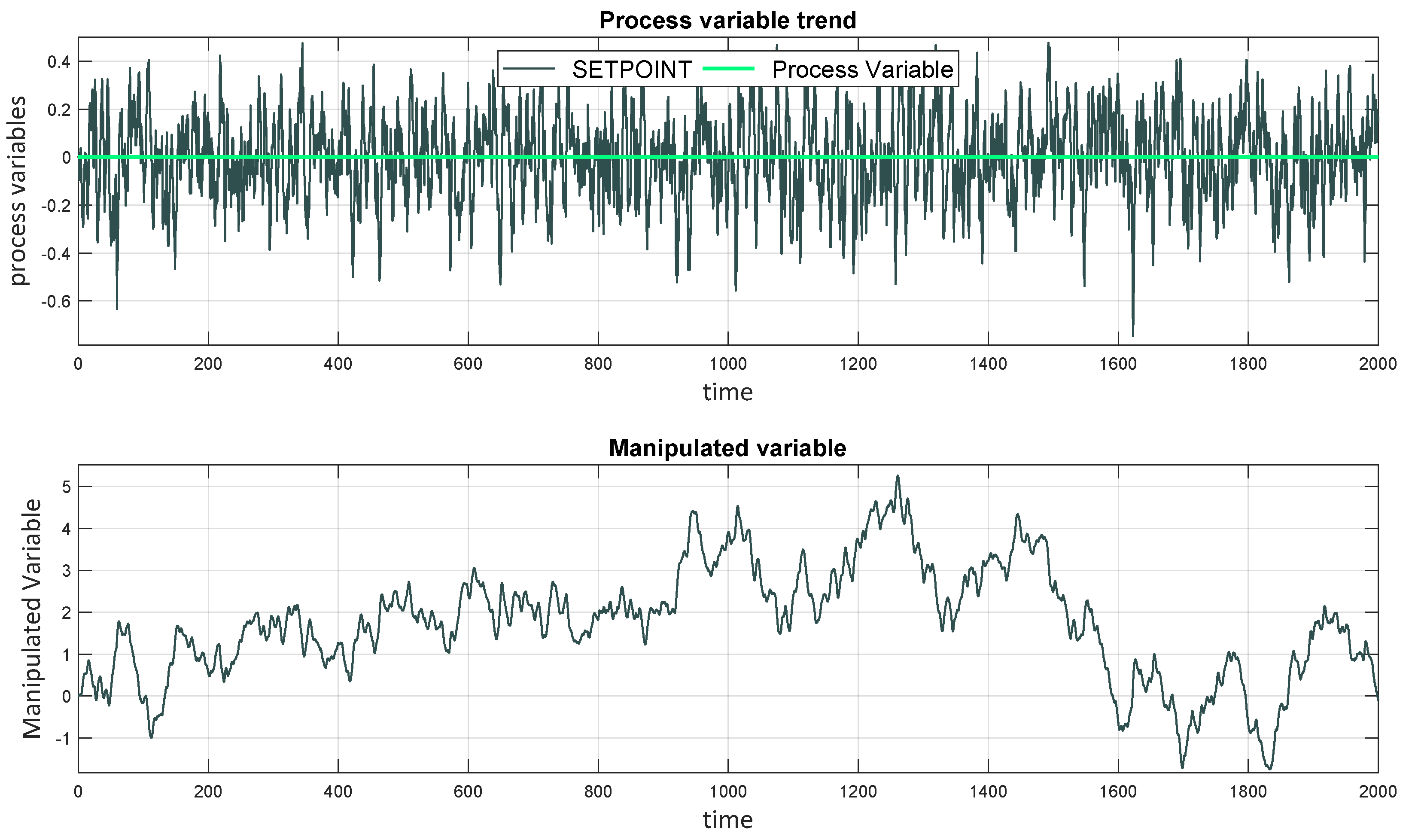
Figure 3 shows sample trends for the G 1 ( s ) controlled by the well-tuned PID k p = 1.050 , T i = 2.998 , T d = 0.929 . The good PID for G 4 ( s ) has k p = 0.265 , T i = 0.607 ,   T d = 0.212 , and for G 5 ( s ) k p = 0.133 , T i = 0.259 , T d = 0.081 .
The analysis uses various PID parameter sets. The gain k p 0.05 ; 2.05 changes every 0.25 , the integration time T i 0.2 ; 10.2 changes every, 1.0 and the T d = const = 0.9293 . To exclude statistical effects, each set of parameters is run 20 times and the resulting CPA measures are averaged. The same approach is repeated for the other two transfer functions. For G 4 ( s ) , the k p 0.2 ; 1.6 changes every 0.2 , the T i 0.1 ; 5.1 changes every 0.5 and the T d = const = 0.2121 . For G 5 ( s ) , the k p 0.02 ; 1.02 changes every 0.1 , the T i 0.05 ; 2.3 changes every 0.25 , and the T d = const = 0.0808 .

3.1. Simulation Results

The conducted simulation experiments and the associated results are presented in the order of the analyses conducted and the next steps follow directly from the previous observations. It is assumed that such an arrangement will aid the reader in understanding not only the results but also how they were acquired.
The full layout of the analysis is presented for the first plant G 1 ( s ) , while subsequent transfer functions allow us to visualize the observations made for the first one.
Historically, and also practically, the loop step response overshoot κ and the settling time T set are the most popular and commonly understood control performance measures [37]. The overshoot addresses loop oscillations. We often require a zero overshoot value, but this might not be achievable. The higher the κ is, the worse the loop performance is. Control tuning exhibiting a high overshoot value is deemed aggressive. The settling time reflects how quickly the loop settles after step occurrence. The ultimate goal is for T set to be as short as possible, to achieve the fastest response, as its high values reflect very long responses (sluggish control).
Overshoot has the opposite meaning to the settling time. We cannot achieve zero overshoot and very short settling times at the same time. Higher overshoot results in lower T set values and vice versa. Controller design is a form of multicriteria problem. Even this basic and historical example shows the need for multicriteria control system assessment.
Following the above short introduction, the comparison of the energy indexes in relation to the κ and the T set seems to provide the best starting point for analysis. Figure 4a shows the relationship between the overshoot and settling time IRD( κ , T set ) for the G 1 ( s ) plant. The shading of the circles is in line with the quadratic manipulated variable MV 2 and thus it reflects how the energy spent on control actions relates to the loop performance.
Additionally, the picture is scaled to obtain an equalized relation between the values on both coordinates. It is scaled using the following coefficients: x m a x = 80 and y m a x = 900 . The points create a form of Pareto front of the possible multicriteria optimal solutions.
We see that the lowest control energy (blue diamond) is obtained for the extremely sluggish control. Its value equals 0.02 . In contrast, the highest obtained MV 2 = 46.57 . The tuning closest to the origin (zero κ and T set ) gives MV 2 = 2.01 . It is worth mentioning that this point relates to the following tuning: k p = 1.05 and T i = 3.20 .
As one can see, the energy consumed for the realization of the controller output spans a wide range, MV 2 0.02 ; 46.57 . Figure 4b presents the same relationship but is magnified to better show the region close to the origin.
The next two plots show an analogous relation, but related to the valve travel in Figure 5a and valve stroke indexes in Figure 5b. We observe that the valve stroke behaves in a similar way to the valve energy; however, its variability is more uniform and K VT 14.6 ; 759.1 with an optimal value equal to 173.5 . This point relates to k p = 1.05 and T i = 2.20 .
The valve stroke index behaves in an unusual way as it reflects rapid and high-frequency oscillations in the control signal. It varies in a very wide range, K VS 297 ; 6432 . Its interpretation is rather non-intuitive. High-performance controllers are characterized by high valve stroke values as they tend to reach the setpoint in small oscillations, i.e., frequently changing the stroke direction. The best stroke results are obtained for small settling times, but relatively high (and probably not acceptable) overshoots.
As a result of the above analysis, the valve travel index K VT is selected as a representative of the controller output energy. The following figures show how the valve travel index relates to the other loop performance indexes. The analysis aims at finding the most representative combinations of the performance indicators that could be practically used in control assessment studies.
This stage of the analysis starts with the comparison of the two most popular integral indexes (MSE and MAE) with the K VT in the two-criteria IRD plots. Figure 6a shows the IRD (MSE, K VT ) relationship and is shaded according to the MAE index. It exhibits the following scaling coefficients: x m a x = 2.5 and y m a x = 800 . Figure 6b presents the opposite situation for the IRD (MAE, K VT ) plot shaded according to the MSE. It is scaled using x m a x = 1.2 and y m a x = 800 .
The IRD (MSE, K VT ) relationship points out the following tuning: k p = 0.3 and T i = 3.20 . Meanwhile, the IRD (MAE, K VT ) prefers the more sluggish combination of k p = 0.8 and T i = 3.20 .
Initially, both plots appear very similar. The Pareto front is visible, and the poor tuning, denoted by high MSE or MAE values, is located in the aggressive control section of the diagram. A difference starts to appear at low index values. We see that the MAE version shown in Figure 6b allows the more precise distinction of different parameter settings for good controllers. This perspective, combined with the higher robustness of the MAE to outliers, indicates another choice. The mean absolute measure will be treated as a distinguisher of control quality in subsequent diagrams.
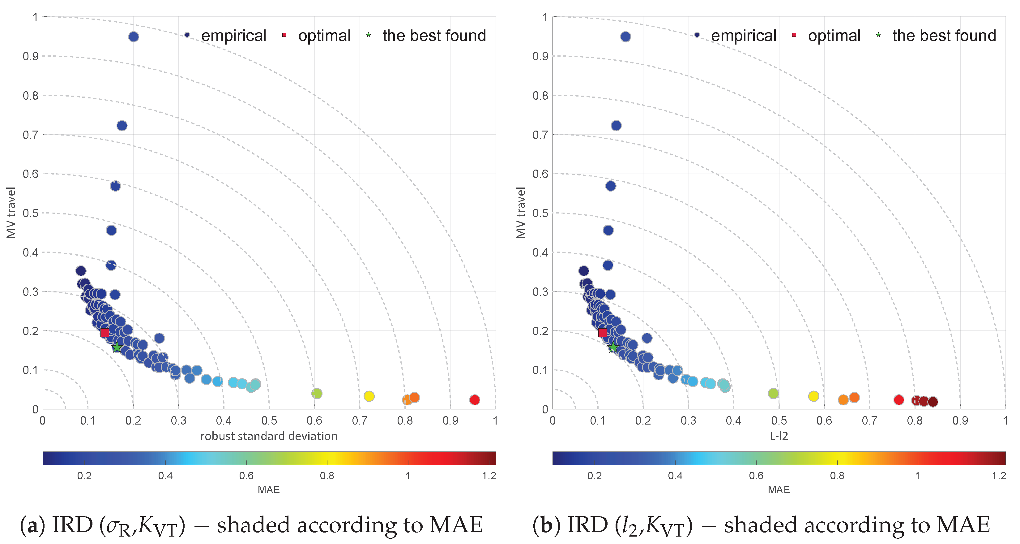
The consecutive analyses use shading according to the MAE index, while the loop performance indicator is replaced. The next two diagrams use different statistical scale estimators as measures of the loop performance. Figure 7a incorporates the robust standard deviation estimator σ R in the form of the IRD ( σ R , K VT ) diagram. Figure 7b uses the L-scale estimator l 2 in the form of the IRD ( l 2 , K VT ).
Both plots are almost identical, as both scale estimators exhibit similar features and are quite equivalent. Thus, it is not surprising that both indicate the same controller to be the best as in case of the IRD (MAE, K VT ), i.e., k p = 0.8 and T i = 3.20 . The IRD ( σ R , K VT ) is scaled with x m a x = 1.4 and y m a x = 800 and the IRD ( l 2 , K VT ) uses x m a x = 1.0 and y m a x = 800 . At this point in the analysis, we may state that the MAE, σ R , and l 2 are equivalent and, as such, only one of them can be practically used in assessment studies. The MAE is more common and easier to use in evaluations, and it is thus suggested as a representative loop performance indicator.
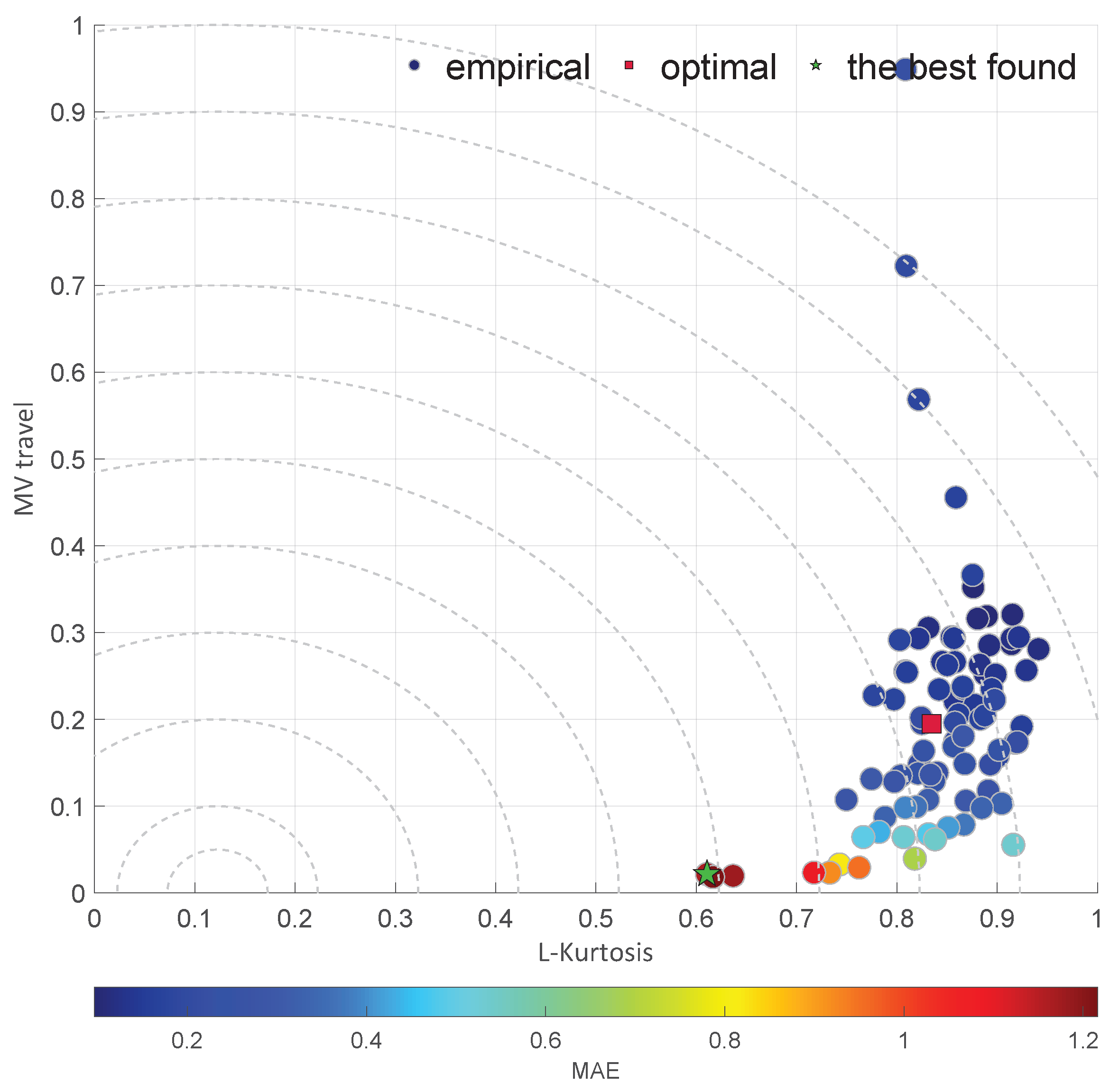
Figure 8 uses as the loop indicator the L-moment estimator of kurtosis, i.e., the L-kurtosis τ 4 . The plot is scaled according the the following limits: x m a x = 0.16 and y m a x = 800 . It should be noted that the selection of the proper L-kurtosis from the perspective of the loop performance is not simple, as it is not zero. As we agree with the assumption that good control should result in the normal distribution of the control signal, the selection of τ 4 = 0.1226 (characteristic value for Gaussian signal) seems to be justified.
We see that the L-kurtosis is not sufficient to fulfil the task of reflecting the quality of control. Although its statistical interpretation seems to be useful, our analysis rather raises skepticism. The IRD ( τ 4 , K VT ) diagram points out k p = 0.05 and T i = 7.20 , which is extremely slow and a very safe choice.
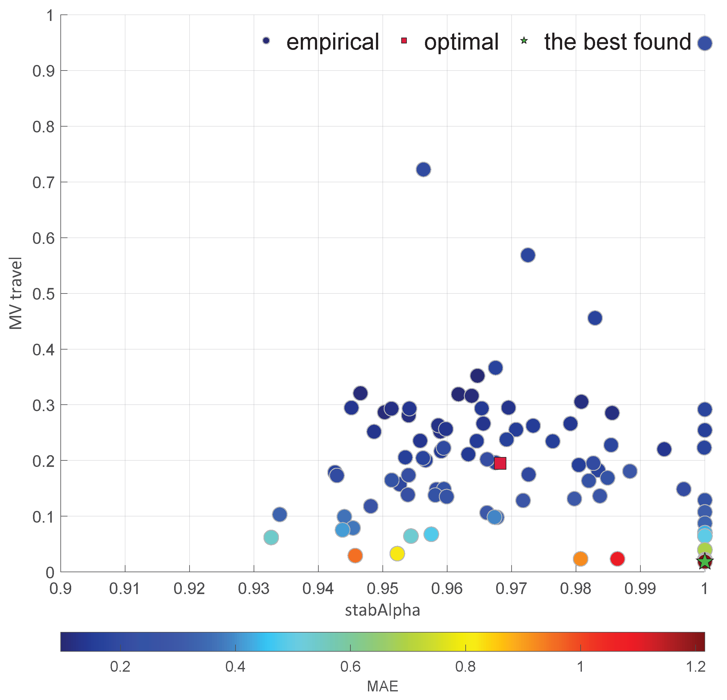
Another non-standard performance indicator choice is shown in Figure 9. It uses the stability exponent coefficient of the α -stable distribution denoted as α for the IRD ( α , K VT ) diagram. It is scaled according to the following limits: x m a x = 2.0 and y m a x = 800 . In contrast, the good control selection of α = 2.0 is also justified in this case as it reflects Gaussian properties.
Following the above assumption, the controller with k p = 0.05 and T i = 10.20 is indicated as the best, which is even more sluggish.
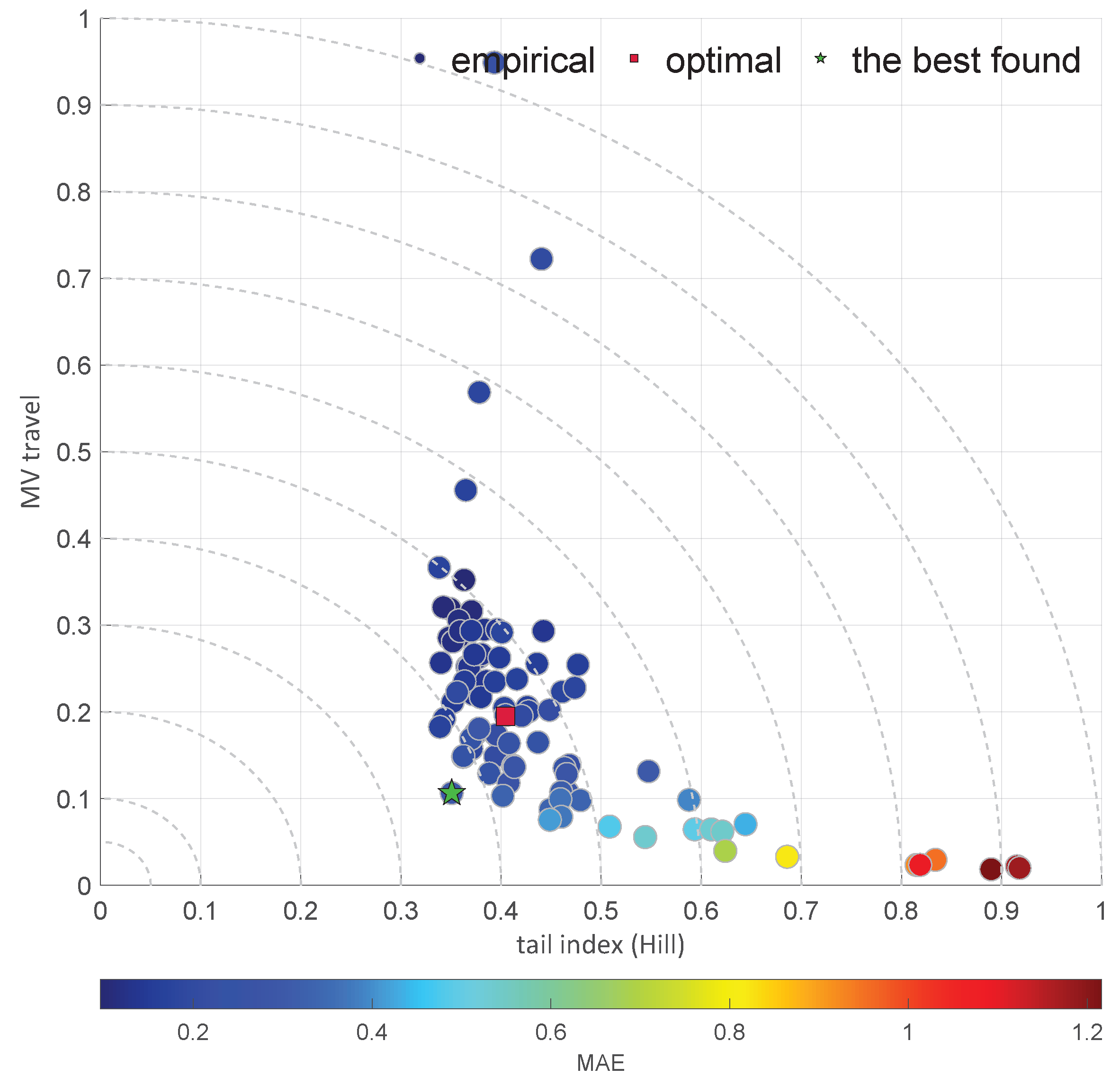
The last two diagrams do not present an obvious choice. Figure 10 uses the tail index ξ ^ as the loop performance estimator, while Figure 11 utilizes the Geweke–Porter–Hudak fractional order estimator d GPH of the potential ARFIMA filter. The tail index is not yet reported in the literature to be used in this context, while the d GPH has been reported only in [38]. The IRD ( ξ ^ , K VT ) diagram is scaled with x m a x = 16.0 and y m a x = 800 and the IRD ( d GPH , K VT ) using x m a x = 1.0 and y m a x = 800 .
It is interesting to note that the tail index used as the loop performance indicator performs according to our expectations. The Pareto-like front is highly visible and the various forms of PID tuning are easily distinguishable. It points out the aggressive controller with k p = 0.30 and T i = 2.20 .
The last is the IRD ( d GPH , K VT ) diagram. According to theory, a good controller should be closer to the point (0, 0), as d GPH = 0 represents independent noise realization, which could be interpreted as a normal property. The IRD ( d GPH , K VT ) diagram indicates a slightly less aggressive controller with k p = 0.30 and T i = 1.20 .
A hypothesis [39] posits that good control should exhibit a control error Hurst exponent value H 0.5 , where smaller values indicate aggressive operation and higher ones indicate sluggish operation. As there is a relationship in which H = d + 0.5 , d = 0 indicates good, 0.5 > d > 0 aggressive, and 0 > d > 0.5 sluggish control. We also observe situations whereby d 0.5 . This means that the process seems to be behave in a non-stationary manner, and it possesses infinite variance. We can interpret this in control engineering to indicate that the controller is extremely sluggish, with almost no reaction to the controller output.
We see that the IRD ( d GPH , K VT ) diagram brings a new dimension. It not only indicates the quality of the loop performance, but also suggests actions to be taken, i.e., to tune the controller towards aggressive or sluggish behavior. A comparison of the results obtained throughout the above analysis is given in Table 1.
The above analysis is provided for one G 1 ( s ) plant. Next, it is extended to two other processes. The description starts with the summary tables, followed by the presentation of the most representative figures. Table 2 summarizes the results obtained for G 4 ( s ) .
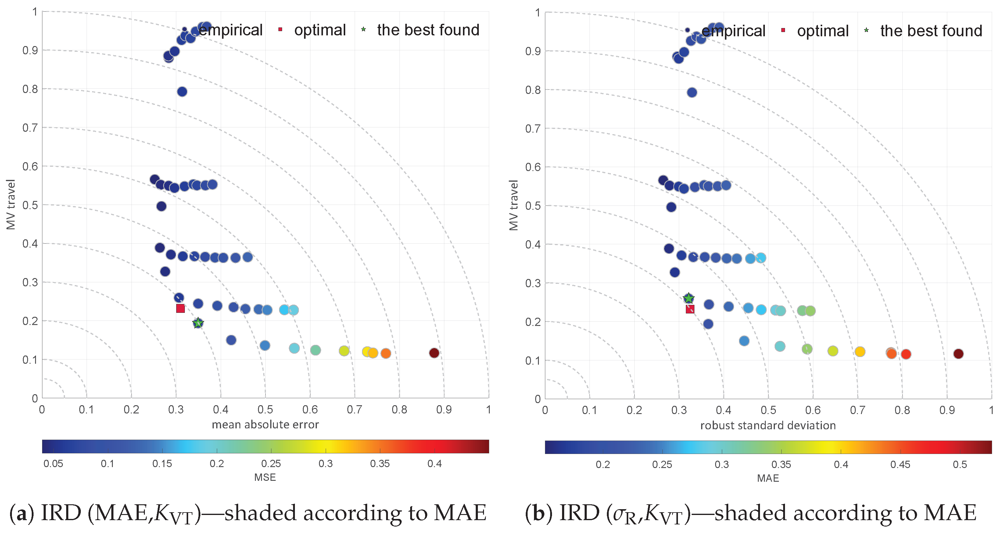
Four representative plots are sketched, according to the results shown in Table 2. Figure 12a shows the IRD (MAE, K VT ) diagram, while Figure 12b the IRD ( σ R , K VT ) diagram. The difference between these two charts is subtle. They both appear almost identical; however, it is likely that the effect of the subtle difference in choosing the best solution depends on this and not the choice of scaling factors. In this example, we can see that this choice matters; however, analogously to the task of the threshold choice, it is strongly subjective and there is unlikely to be a universal tool. Fortunately, the difference in indications is small and the impact on the evaluation in this situation would also be small.
The next two diagrams show the IRD ( ξ ^ , K VT ) in Figure 13a and the IRD ( d GPH , K VT ) in Figure 13b. They appear quite similar, and they suggest the same solution.
Finally, Table 3 presents the respective comparison of the results for plant G 5 ( s ) .
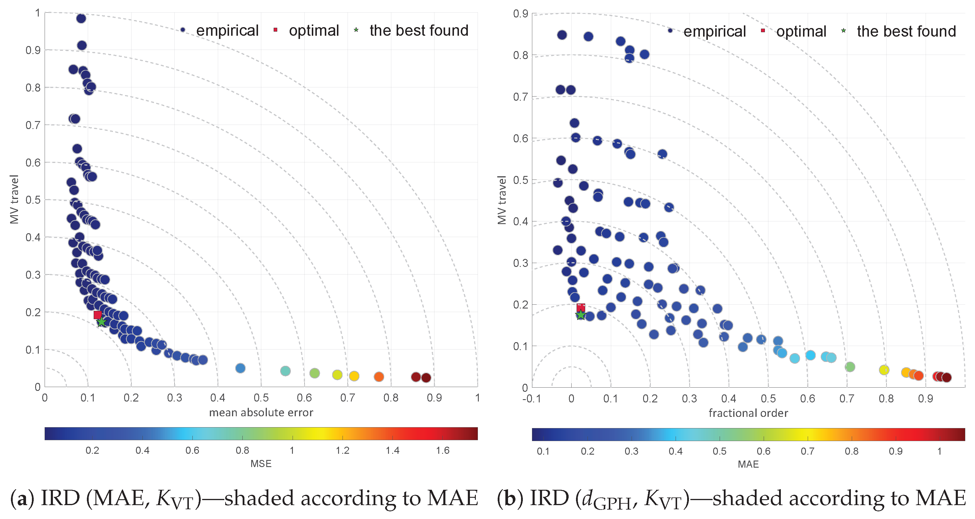
Two representative plots are sketched for the G 5 ( s ) plant. Figure 14a presents the index ratio diagram that uses the MAE index—IRD (MAE, K VT )—while the IRD ( d GPH , K VT ) diagram utilizing the fractional order estimator is shown in Figure 14b. We can clearly see, similarly to the previous transfer functions, the Pareto front of multicriteria solutions and the higher resolution visible in the IRD ( d GPH , K VT ) chart.

3.2. Observations Summary

Three representative plans utilized in single-loop PID control are assessed. Observing the results, we can make the following conclusions.
  • PID loop control quality assessment is a multicriteria task.
  • The overshoot and settling time indexes allow us to deliver a suitable solution, but they exhibit one significant deficiency, as they require a step response, which is not achievable in the industrial reality.
  • The CPA indexes do not take into account the energy spent during control actions and the respective indicators are proposed.
  • The incorporation of the energy factors into the assessment has the tendency to suggest slower controllers, which is natural.
  • The MAE and robust scale estimators behave in a similar way.
  • The shape factors, i.e., the stability exponent α and L-kurtosis τ 4 , have a tendency to indicate extremely sluggish control performance.
  • The use of the fractional order d GPH evaluated as the the Geweke–Porter–Hudak estimator brings a new assessment perspective and enables us to give constructive loop tuning indications.
The above observations should initiate a discussion on the importance of the energy self-consumption by the control algorithm (system) itself. The given control strategy not only affects the process (plant, installation), but it is always obtained at some cost. We can measure this impact as the energy consumed by the control system. Historically, this part of the control loop has been perceived from the perspective of the actuator’s ability to realize the obtained controller output and further by its wear and tear. The valve travel index has been proposed and used to address this issue. The introduction of the energy self-consumption into the picture adds a new perspective and enables the control system to become energy-aware at all levels, even marginal ones.
The search for energy that can be spared has only recently started. Control engineers should consider this during the design and tuning phases. More importantly, plant owners should require them to take into account this energy awareness. However, it must be remembered that this energy minimization is not unconditional. In some cases, an exemplary amount of 1 kW might be achieved at a 10 kW cost in the plant’s performance. In such a case, it is negligible. Because of this, multicriteria IRD diagrams should be used, as they allow us to compare and assess the outcomes.

4. Conclusions and Further Research

This article considers an element that is rarely included in control system energy efficiency analyses, i.e., the energy spent on the realization of control actions. Although this energy amount might be marginal for a single-loop system, especially compared to the cost of the product energy flowing in the process, it starts to be visible in the case of large-scale multi-loop systems.
It is shown that the valve travel or the travel index can fairly represent this energy. The incorporation of this factor into the loop assessment analysis slightly changes the priorities of the control task. The combination of the K VT index with other control performance indicators allows us to perform multicriteria assessment. It is suggested and shown that the use of index ratio diagrams makes this analysis easier in consideration of practitioners.
Ten control performance indicators (MAE, MSE, robust standard deviation σ R , L-scale l 2 , L-kurtosis, tail index ξ ^ , fractional order estimator d GPH , quadratic manipulated variable, valve travel, and valve stroke index) were analyzed. It was shown that the utilization of the simple mean absolute error (MAE) index or another robust scale estimator, together with the K VT , enables us to deliver reasonable results. However, the most interesting result was obtained with the use of the fractional order ARFIMA filter estimator evaluated using the Geweke–Porter–Hudak estimator d GPH . The IRD ( d GPH , K VT ) diagrams not only provided good controllers, but also allowed us to suggest which tuning was required to improve the control performance.
The incorporation of energy awareness into control engineering is quite a new issue and a new challenge. The existing interpretation of the energy consumption by systems is connected with the considered processes directly, and the control system is considered to be an addendum, which consumes some energy but at negligible amounts. Now, the global economy is changing and energy is starting to be treated as a rare and precious resource. While looking for energy limitations, even marginal ones, the energy utilized by the control system itself represents a natural first step. It is necessary to be able to measure it, to asses its impact, and to identify the factors that are responsible for it. Henceforth, we must consciously take this energy into account and manage and minimize the energy consumed by the control system itself.
This work highlights the above problem, proposes an index that allows us to measure this energy, and suggests methods that allow us to assess it and compare it with the control system’s performance. These results are very important, as they can support site engineers during their daily operations. It must be noted that this work is only an initial step towards further research, which should focus on practical systems and not only simulated processes.

Funding

This research received no external funding.

Institutional Review Board Statement

Not applicable.

Data Availability Statement

The data presented in this study are available on request from the corresponding author.

Conflicts of Interest

The author declares no conflicts of interest.

Abbreviations

The following abbreviations are used in this manuscript:
CPAControl Performance Assessment
PIDProportional-Integral-Derivative
KPIKey Performance Indicators
QMVQuadratic Manipulated Variable
MRDMoment Ratio Diagram
LMRDL-Moment Ratio Diagram
IRDIndex Ratio Diagram
MSEMean Square Error
MAEMean Absolute Error
PDFProbability Density Function
MLMaximum Likelihood
GLOGeneralized Logistic distribution
GAMGamma Distribution
LGNLognormal Distribution
EXPExponential Distribution
WEIWeibull Distribution
GEVGeneralized Extreme Value Distribution
GPDGeneralized Pareto Distribution
K4DFour-Parameter Kappa Distribution
LSLeast Squares
QEQuadratic Error

References

  1. Bauer, M.; Horch, A.; Xie, L.; Jelali, M.; Thornhill, N. The current state of control loop performance monitoring—A survey of application in industry. J. Process Control 2016, 38, 9539. [Google Scholar] [CrossRef]
  2. O’Neill, Z.; Li, Y.; Williams, K. HVAC control loop performance assessment: A critical review (1587-RP). Sci. Technol. Built Environ. 2017, 23, 619–636. [Google Scholar] [CrossRef]
  3. Mercorelli, P. Robust Control as a Mathematical Paradigm for Innovative Engineering Applications. Mathematics 2022, 10, 4399. [Google Scholar] [CrossRef]
  4. Liberati, F.; Cirino, C.M.F.; Tortorelli, A. Energy-Aware Model Predictive Control of Assembly Lines. Actuators 2022, 11, 172. [Google Scholar] [CrossRef]
  5. Arabas, P.; Sikora, A.; Szynkiewicz, W. Energy-Aware Activity Control for Wireless Sensing Infrastructure Using Periodic Communication and Mixed-Integer Programming. Energies 2021, 14, 4828. [Google Scholar] [CrossRef]
  6. Krok, M.; Majewski, P.; Hunek, W.P.; Feliks, T. Energy Optimization of the Continuous-Time Perfect Control Algorithm. Energies 2022, 15, 1555. [Google Scholar] [CrossRef]
  7. Domański, P.D. Improving Actuator Wearing Using Noise Filtering. Sensors 2022, 22, 8910. [Google Scholar] [CrossRef]
  8. Grobelna, I. Intelligent Industrial Process Control Systems. Sensors 2023, 23, 6838. [Google Scholar] [CrossRef]
  9. Ouarda, T.; Charron, C.; Chebana, F. Review of criteria for the selection of probability distributions for wind speed data and introduction of the moment and L-moment ratio diagram methods, with a case study. Energy Convers. Manag. 2016, 124, 247–265. [Google Scholar] [CrossRef]
  10. Chaber, P.; Domański, P.D. Control Assessment with Moment Ratio Diagrams. In Proceedings of the Advanced, Contemporary Control; Pawelczyk, M., Bismor, D., Ogonowski, S., Kacprzyk, J., Eds.; Springer: Cham, Switzerland, 2023; pp. 3–13. [Google Scholar]
  11. Kaniuka, J.; Ostrysz, J.; Groszyk, M.; Bieniek, K.; Cyperski, S.; Domański, P.D. Study on Cost Estimation of the External Fleet Full Truckload Contracts. In Proceedings of the 20th International Conference on Informatics in Control, Automation and Robotics, Rome, Italy, 13–15 November 2023; Volume 2, pp. 316–323. [Google Scholar]
  12. Huber, P.J.; Ronchetti, E.M. Robust Statistics, 2nd ed.; Wiley: Hoboken, NJ, USA, 2009. [Google Scholar]
  13. Hosking, J.R.M. L-Moments: Analysis and Estimation of Distributions Using Linear Combinations of Order Statistics. J. R. Stat. Soc. Ser. B 1990, 52, 105–124. [Google Scholar] [CrossRef]
  14. Qi, Y. On the tail index of a heavy tailed distribution. Ann. Inst. Stat. Math. 2010, 62, 277–298. [Google Scholar] [CrossRef]
  15. Sheng, H.; Chen, Y.; Qiu, T. Fractional Processes and Fractional-Order Signal Processing; Springer: London, UK, 2012. [Google Scholar]
  16. Liu, K.; Chen, Y.; Zhang, X. An Evaluation of ARFIMA (Autoregressive Fractional Integral Moving Average) Programs. Axioms 2017, 6, 16. [Google Scholar] [CrossRef]
  17. Samad, T. A Survey on Industry Impact and Challenges Thereof [Technical Activities]. IEEE Control Syst. Magaz. 2017, 37, 17–18. [Google Scholar]
  18. Åström, K.J.; Hägglund, T. Benchmark Systems for PID Control. In Proceedings of the IFAC Digital Control: Past, Present and Future of PlD Control, Terrassa, Spain, 5–7 April 2000; pp. 165–166. [Google Scholar]
  19. Knierim-Dietz, N.; Hanel, L.; Lehner, J. Definition and Verification of the Control Loop Performance for Different Power Plant Types; Technical Report; Institute of Combustion and Power Plant Technology, University of Stuttgart: Stuttgart, Germany, 2012. [Google Scholar]
  20. Rousseeuw, P.J.; Leroy, A.M. Robust Regression and Outlier Detection; John Wiley & Sons, Inc.: New York, NY, USA, 1987. [Google Scholar]
  21. Bílková, D. L-Moments and TL-Moments as an Alternative Tool of Statistical Data Analysis. J. Appl. Math. Phys. 2014, 2, 919–929. [Google Scholar] [CrossRef]
  22. Peel, M.; Wang, Q.; Mcmahon, T. The utility L-moment ratio diagrams for selecting a regional probability distribution. Hydrol. Sci. J. 2001, 46, 147–155. [Google Scholar] [CrossRef]
  23. Ronchetti, E. The main contributions of robust statistics to statistical science and a new challenge. In Metron; Springer: Berlin/Heidelberg, Germany, 2021; Volume 79, pp. 127–135. [Google Scholar]
  24. Verboven, S.; Hubert, M. LIBRA: A Matlab library for robust analysis. Chemom. Intell. Lab. Syst. 2005, 75, 127–136. [Google Scholar] [CrossRef]
  25. Vargo, E.; Pasupathy, R.; Leemis, L. Moment-Ratio Diagrams for Univariate Distributions. In Computational Probability Applications; Springer: Berlin/Heidelberg, Germany, 2010; Volume 42, pp. 149–164. [Google Scholar]
  26. Tallaksen, L.; Van Lanen, H. Hydrological Drought: Processes and Estimation Methods for Streamflow and Groundwater; Developments in Water Science; Elsevier Science B.V.: Amsterdam, The Netherlands, 2004; Volume 48. [Google Scholar]
  27. Kjeldsen, T.R.; Ahn, H.; Prosdocimi, I. On the use of a four-parameter kappa distribution in regional frequency analysis. Hydrol. Sci. J. 2017, 62, 1354–1363. [Google Scholar] [CrossRef]
  28. Taleb, N.N. Real-World Statistical Consequences of Fat Tails: Papers and Commentary; Technical Incerto Collection; STEM Academic Press: New York, NY, USA, 2018. [Google Scholar]
  29. Fedotenkov, I. A Review of More than One Hundred Pareto—Tail Index Estimators. Statistica 2020, 80, 245–299. [Google Scholar]
  30. Hill, B.M. A Simple General Approach to Inference About the Tail of a Distribution. Ann. Stat. 1975, 3, 1163–1174. [Google Scholar] [CrossRef]
  31. Huisman, R.; Koedijk, K.; Kool, C.; Palm, F. Tail-Index Estimates in Small Samples. J. Bus. Econ. Stat. 2001, 19, 208–216. [Google Scholar] [CrossRef]
  32. Burnecki, K.; Sikora, G. Identification and validation of stable ARFIMA processes with application to UMTS data. Chaos Solitons Fractals 2017, 102, 456–466. [Google Scholar] [CrossRef]
  33. Geweke, J.; Porter-Hudak, S. The Estimation and Application of Long Memory Time Series Models. J. Time Ser. Anal. 1983, 4, 221–238. [Google Scholar] [CrossRef]
  34. Beran, J. Statistics for Long-Memory Processes, 1st ed.; Routledge: New York, NY, USA, 1994. [Google Scholar]
  35. Unbehauen, H. Controller design in time domain. In Encyclopedia of Life Support Systems (EOLSS); Unbehauen, H., Ed.; Eolss Publishers: Oxford, UK, 2009. [Google Scholar]
  36. Nolan, J. Univariate Stable Distributions. Models for Heavy Tailed Data; Springer Series in Operations Research and Financial Engineering; Springer Nature: Cham, Switzerland, 2020. [Google Scholar]
  37. Swanda, A.P.; Seborg, D.E. Controller performance assessment based on setpoint response data. In Proceedings of the 1999 American Control Conference, San Diego, CA, USA, 2–4 June 1999; Volume 6, pp. 3863–3867. [Google Scholar]
  38. Chaber, P.; Domański, P.D. Fractional control performance assessment of the nonlinear mechanical systems. In Proceedings of the Preprints of the 3rd International Nonlinear Dynamics Conference NODYCON 2023, Rome, Italy, 18–22 June 2023. [Google Scholar]
  39. Spinner, T.; Srinivasan, B.; Rengaswamy, R. Data-based automated diagnosis and iterative retuning of proportional-integral (PI) controllers. Control Eng. Pract. 2014, 29, 23–41. [Google Scholar] [CrossRef]
Figure 1. L-moment diagram for theoretical PDFs. Red line depicts the lower band. Grey color covers K4D area.
Energies 17 01173 g001
Figure 2. Environment for the experiments.
Energies 17 01173 g002
Figure 3. Time series for loop G 1 ( s ) and optimal PID tuning.
Energies 17 01173 g003
Figure 4. IRD ( κ , T set ) diagram for G 1 ( s ) : red square depicts good tuning, green star the best found, blue diamond the lowest MV 2 (circles are shaded according to quadratic manipulated variable MV 2 ).
Energies 17 01173 g004
Figure 5. IRD ( κ , T set ) diagram for G 1 ( s ) : red square depicts good tuning, green star the best found, blue diamond the lowest valve index.
Energies 17 01173 g005
Figure 6. IRD diagrams for G 1 ( s ) : red square depicts good tuning, green star the best found.
Energies 17 01173 g006
Figure 7. IRD diagrams for G 1 ( s ) : red square depicts good tuning, green star the best found.
Energies 17 01173 g007
Figure 8. Scaled IRD ( τ 4 , K VT ) diagram for G 1 ( s ) .
Energies 17 01173 g008
Figure 9. Scaled IRD ( α , K VT ) diagram for G 1 ( s ) .
Energies 17 01173 g009
Figure 10. Scaled IRD ( ξ ^ , K VT ) diagram for G 1 ( s ) .
Energies 17 01173 g010
Figure 11. Scaled IRD ( d GPH , K VT ) diagram for G 1 ( s ) .
Energies 17 01173 g011
Figure 12. IRD diagrams for G 4 ( s ) : red square depicts good tuning, green star the best found.
Energies 17 01173 g012
Figure 13. IRD diagrams for G 4 ( s ) : red square depicts good tuning, green star the best found.
Energies 17 01173 g013
Figure 14. IRD diagrams for G 5 ( s ) : red square depicts good tuning, green star the best found.
Energies 17 01173 g014
Table 1. Summary of the analysis for the G 1 ( s ) plant.
Diagram k p T i T d κ T set Characteristic
IRD ( κ , T set )1.053.200.92930.019.47good
IRD (MSE, K VT )0.303.200.92930.0038.7sluggish
IRD (MAE, K VT )0.803.200.92930.0012.60good
IRD ( l 2 , K VT )
IRD ( τ 4 , K VT )0.057.200.92930.00572extremely sluggish
IRD ( α , K VT )0.0510.200.92930.00816extremely sluggish
IRD ( ξ ^ , K VT )0.302.200.92930.0020.7good, slow
IRD ( d GPH , K VT )0.301.200.929314.9825.5aggressive
Table 2. Summary of the analysis for the G 4 ( s ) plant.
Diagram k p T i T d κ T set Characteristic
IRD ( κ , T set )0.601.100.21210.006.92good
IRD (MSE, K VT )0.200.600.21210.008.73good
IRD (MAE, K VT )
IRD ( σ R , K VT )0.401.100.21210.0010.00slow
IRD ( l 2 , K VT )
IRD ( τ 4 , K VT )0.205.100.21210.00111extremely sluggish
IRD ( α , K VT )0.203.600.21210.0076.9extremely sluggish
IRD ( ξ ^ , K VT )0.200.600.21210.008.73good
IRD ( d GPH , K VT )0.200.600.21210.008.73good
Table 3. Summary of the analysis for the G 5 ( s ) plant.
Diagram k p T i T d κ T set Characteristic
IRD ( κ , T set )0.320.550.08081.234.56fast
IRD (MSE, K VT )0.120.550.08080.0016.15slow
IRD (MAE, K VT )0.220.550.08080.027.84good
IRD ( σ R , K VT )
IRD ( l 2 , K VT )
IRD ( τ 4 , K VT )0.022.300.08080.00453.00extremely sluggish
IRD ( α , K VT )
IRD ( ξ ^ , K VT )0.220.300.08085.646.55aggressive
IRD ( d GPH , K VT )0.020.050.08081.665.82fast
Disclaimer/Publisher’s Note: The statements, opinions and data contained in all publications are solely those of the individual author(s) and contributor(s) and not of MDPI and/or the editor(s). MDPI and/or the editor(s) disclaim responsibility for any injury to people or property resulting from any ideas, methods, instructions or products referred to in the content.