Abstract
Flooded Lead Acid (FLA) batteries remain a cost-effective choice in various industries. Accurate State of Charge (SOC) estimation is crucial for effective battery management systems. This paper thoroughly examines the behavior of Open-Circuit Voltage (OCV) during hysteresis in FLA batteries, proposing a novel hysteresis modeling approach based on this behavior to enhance the SOC estimation accuracy. Additionally, we introduce an Adaptive Unscented Kalman Filter (AUKF) to further refine the SOC estimation precision. Experimental validation confirms the effectiveness of the proposed hysteresis modeling. A comparative analysis against the traditional Unscented Kalman Filter (UKF) under random charge/discharge profiles underscores the superior performance of AUKF, showcasing an improved convergence to the correct SOC value and a significant reduction in the SOC estimation error to approximately 2%, in contrast to the 5% error observed with the traditional UKF.
1. Introduction
Energy storage systems are very popular in the industry due to their increased demand in a number of applications, from smart micro grids to electrified transportation systems [1]. Among these energy storage systems, batteries receive the most attention because of their wide range of power and energy densities and low cost as compared to other systems such as flywheels, ultra-capacitors, or hydrogen storage [2]. There are different types of batteries available in the market like Li Ion, lead acid, and nickel cadmium, etc. Among lead acid batteries, Flooded Lead Acid (FLA) batteries are a versatile and dependable choice in numerous applications, including backup power systems, automotives, renewable energy storage, and aviation [3]. Their enduring appeal lies in their cost-effectiveness, reliability, and adaptability, making them a reliable energy storage solution across a broad spectrum of industries.
The State of Charge (SOC) estimation of a battery is one of the fundamental requirements of a battery management system. SOC estimation becomes a critical concern in extending battery lifetime, preventing progressive unalterable damage, and enhancing battery operation performance; therefore, a proper analysis of the internal behavior of Sealed Flooded Lead Acid (SFLA) batteries for SOC estimation is required, as this has not been conducted before. A battery management system (BMS) is an application which uses a suitable equivalent model for the battery to protect it from over-voltages and over-currents and estimates the other required states of the battery like the SOC, State of Health (SOH), and State of Function (SOF), etc. [4,5,6]. As the Open-Circuit Voltage (OCV) is computed through the SOC input and SOC–OCV relationship, then combining it with the battery polarization voltage can be used to model the battery dynamics. The SOC–OCV relationship is very important in the modeling of the battery equivalent circuit, since equivalent circuit models make the complex electrochemical processes occurring within a battery simpler by representing them with electrical components like resistors, capacitors, and voltage sources. The SOC–OCV relationship is key in determining the voltage source within this model. By obtaining an accurate SOC–OCV relationship, the equivalent circuit model can effectively mimic how the battery voltage changes during charging and discharging cycles. The relation of SOC–OCV is not simply a one-to-one mapping, but it exhibits the hysteresis effect (the OCV is different at the same SOC value depending upon the history of charge and discharge). Normally, the hysteresis effect is not very effective in most Li-Ion batteries like lithium manganese oxide and lithium cobalt, etc. [4]. This is because the gap between the SOC–OCV charge and discharge curves is very small in most of the region. But the hysteresis effect is very prominent in lead acid batteries, especially in SFLA batteries [7]. The low nominal cell voltage of lead acid batteries, changes in charging rates, and the effects of aging contribute to the prominence of the hysteresis effect. Understanding and addressing this effect is crucial for accurate SOC estimation and applicable battery management in applications using lead acid batteries. Therefore, accurately modeling the hysteresis phenomenon in FLA batteries is essential for achieving accurate SOC estimation results.
To model the hysteresis effect of batteries, different approaches have already been published. For those batteries in which the hysteresis effect is not very dominant, an average of the charge and discharge curves is used as the SOC–OCV relationship. This type of approximation will create a large SOC estimation error for those batteries which have a significant hysteresis phenomenon. Sirinivasan et al. proposed an empirical approach to model hysteretic curves based on the boundary curves of hysteresis in nickel hydroxide electrode, and the process worked well in predicting how the battery discharged, but it was not as accurate when predicting how it charged [8]. Verbrugge et al. formulated a first-order differential equation to construct voltage behavior for NiMH batteries [9]. Roscher et al. modeled the hysteresis of a battery by using a parallelogram [10]. Thele et al. formulated second-order polynomial equations to model the shapes of the hysteresis of NiMH batteries [11]. Similarly, the Takacs model and Preisach model of hysteresis were used in batteries by Windarko et al. and Tang et al., respectively [12,13]. All these hysteresis models are based on the fact that the hysteresis loop always touches the SOC–OCV charge curve whenever it is applied from the SOC–OCV discharge curve and vice versa. The hysteresis phenomenon in maintenance-free SFLA batteries has not been investigated before; therefore, the behavior of the OCV requires both proper investigation and modeling according to its behavior. The proposed research is unique in the sense that it fully investigates the OCV behavior and proposes a novel hysteresis model for SFLA batteries.
An online estimation of the parameters of an equivalent model of battery is very important for making the battery model more and more accurate. In this research, an Auto Regression for external Input (ARX) model for the battery combined with the Recursive Least Squares (RLS) method is used for the parameters’ estimations. The ARX model is a type of linear system model used to describe the relationship between the input and output of a dynamic system. It is often used for modeling and control applications. In the context of battery modeling, the ARX model represents the behavior of a battery as a linear combination of past inputs and outputs. The model assumes that the current output is a linear function of previous inputs and outputs, as well as external input signals. Various methods can be used for parameter estimation, and one of the common techniques is the RLS method. RLS is an adaptive filter algorithm used for estimating the parameters of a linear model. It is particularly useful when dealing with time-varying systems and noisy data. RLS updates the parameter estimates iteratively as new data become available. RLS minimizes the sum of squared errors between the observed output and the predicted output of the model. The algorithm recursively updates the parameter estimation by giving more weight to recent data and less weight to older data. The OCV information from the SOC estimation algorithm is sent to the ARX model, which estimates the values of the parameters by the RLS method and provides the parameters back to the SOC estimation algorithm. So, both the parameter estimation algorithm and the SOC estimation algorithm work in parallel and exchange information at every iteration [14].
For the SOC estimation of a battery, different estimation algorithms are proposed, such as Artificial Neural Networks (ANNs) that control complex neural structures for accurate predictions, ampere-hour counting which integrates the current flow to estimate the SOC, Kalman filters that balance mathematical models and measurements for real-time SOC tracking, and fuzzy logics, which provide a robust, rule-based approach to SOC estimation, etc. Among them, Kalman filters have received the most attention because of their simplicity and accuracy. Kalman filters are usually used for linear systems. For non-linear systems, the Extended Kalman Filter (EKF) was developed, which uses Tylor Series Expansion to linearize any system across a certain point. As batteries are also very non-linear in their behavior, EKFs are widely adopted by most researchers for their SOC estimation. Recently, the Unscented Kalman Filter (UKF) was developed to further improve the estimation accuracy when estimating the state of a non-linear system, surpassing the capabilities of the EKF. While the EKF relies on linear approximations for non-linear systems, which can introduce errors, the UKF takes a more robust approach. It employs a deterministic sampling technique that captures a set of representative points, or sigma points, from the probability distribution of the state variables of the system [15,16,17,18,19,20,21].
In a Kalman filter, process and measurement noise covariances play a vital role in the calculation of filter gain. Unfortunately, there is not any rule of thumb available for finding the values of these noises for any given system. Mostly, these noises are selected based on a trial-and-error method. In practical systems, especially in electric vehicles (EVs), sudden acceleration and deceleration can cause rapid shifts in the dynamics of the battery system. Maintaining constant noise values may result in higher estimation errors, highlighting the need for adaptive approaches that account for these dynamic changes in the system. Similarly, when constant values are used for the covariance of process and measurement noises in a Kalman filter, the Kalman gain, which determines the weight given to the measurement data, becomes constrained to a specific range. This constraint restricts the filter adaptability to varying noise conditions, limiting its ability to respond effectively to unexpected changes in the environment or system dynamics. In such cases, the filter performance may suffer when faced with real-world uncertainties, as it cannot freely adjust the Kalman gain to optimize the state estimation. Therefore, an adaptive system is required which can update the values of the process and measurement noise covariances based on the system error generated in each iteration, giving independence to the Kalman filter to work freely and more accurately in the SOC estimation process [22,23].
In this research, firstly, the most important hysteresis effect of the FLA battery is discussed in detail and, depending upon the results and analysis, a novel hysteresis modeling method is proposed and tested. Secondly, an AUKF method is proposed to optimize the results for a better SOC estimation for FLA batteries. Experimental results are presented to validate the proposed hysteresis model. Similarly, a comparison of simple (traditional) UKF and adaptive UKF is presented, which proves the superiority of adaptive UKF.
2. Hysteresis Effect and Modeling
2.1. Battery Model
The battery electric equivalent circuit consists of an OCV connecting in serial with an internal resistance Ri and an R-C parallel branch of a charge transfer resistance Rct and a double-layer capacitance Cdl to perform the voltage response from the battery current, as shown in Figure 1. This battery model is simple and effective, which means it can be applied easily in practical application. The OCVf is the final OCV, including both the effects of hysteresis and diffusion, due to which, the model becomes very simple and easy to handle for SOC estimation. For parameter estimation, ARX is used, which is essential for accurately determining the parameters that characterize the behavior of the battery, enabling more precise modelling and effective battery management. The details of the ARX method and how to include the hysteresis and diffusion effects in OCV are given in [7,14], respectively.
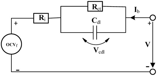
Figure 1.
Selected equivalent circuit of lead acid battery.
2.2. Brief Introduction of Hysteresis Phenomenon
Hysteresis is a phenomenon in which a change in the direction of the independent variable leads to the dependent variable failing to retrace the path it passed in the forward direction. Speaking specifically about electrochemical systems, hysteresis refers to the delayed and non-linear voltage response observed during the charge and discharge cycles of a battery. This phenomenon results from internal chemical and physical processes, such as changes in electrode structure and the formation of compounds, causing a voltage gap between the charging and discharging curves. An accurate estimation of the SOC is complicated due to the hysteresis effect. Understanding and modeling hysteresis is crucial for designing effective battery management systems, predicting battery performance, and optimizing usage in applications ranging from electric vehicles to renewable energy storage systems. Systematic investigations into the nature of the equilibrium potential hysteresis of the nickel electrode by Podolske Ta et al. [24] and Srinivasan et al. [8] led to the following characterization of hysteresis, which could be corroborated by our own measurements:
- The hysteresis is static, i.e., it remains after a charging or discharging current is switched off, even for a period of time that significantly exceeds the time constants of the mass transport inside the electrodes.
- The hysteresis is independent of the preceding current rate.
- The hysteresis is not only characterized by the boundary curves, but also by intermediate sub-hysteresis loops.
These characteristics of hysteresis are in accordance with a domain theory that states that the electrode material is composed of clearly separated regions (domains), each of which exhibits two or more metastable states [8]. The hysteresis phenomenon in FLA batteries is also similar to the above-mentioned batteries.
2.3. Behavior of Hysteresis Loops w.r.t. SOC–OCV Curve
SOC–OCV curves with 3 min (mints) and 3 h (h) of resting are given in Figure 2. Similarly, SOC–OCV curves with different hysteresis loops are shown in Figure 3. All the hysteresis loops are obtained by using 5% SOC pulses with 3 h of relaxation.
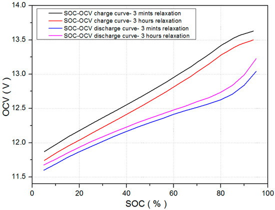
Figure 2.
SOC–OCV curve of FLA battery.
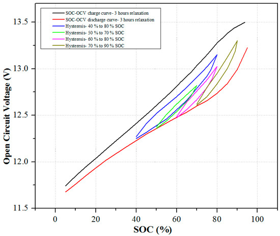
Figure 3.
Different hysteresis curves with SOC–OCV 3 h curves.
As can be clearly observed in Figure 3, the OCV in all the hysteresis loops does not touch the SOC–OCV charge curve.
Even in 40–80% hysteresis loops, the OCV becomes almost parallel to the SOC–OCV charge curve and does not touch it. It clearly shows that, even if this curve is extended, it will not touch the SOC–OCV charge curve.
This phenomenon is quite different from other battery types like Absorbent Glass Mat (AGM), NiMH, or Li-ion, as in all those batteries, the hysteresis loop always touches the SOC–OCV charge curve at some stage. So, this unique behavior requires us to create new hysteresis model for this type of lead acid battery.
2.4. Behavior of Hysteresis OCV at Different SOC Values
It was analyzed that the hysteresis OCV does not touch the SOC–OCV charge curve, regardless of the applied hysteresis loop. In fact, the hysteresis loop becomes parallel to the SOC–OCV charge curve. In Figure 4, hysteresis loops of the 20% SOC range are shifted and shown together. The graph clearly shows that the rate of increase in the OCV is different in different SOC regions. This phenomenon is, in fact, natural, but as there is no range after which the OCV touches the SOC–OCV charge curve, therefore, for the modeling of hysteresis, this phenomenon should be considered.
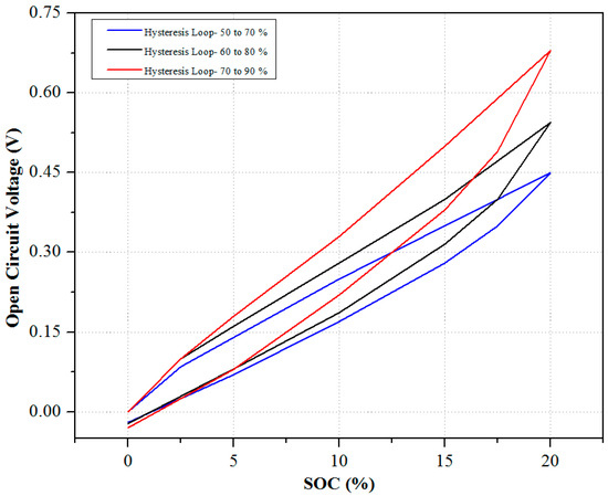
Figure 4.
Shifted hysteresis loops.
2.5. Modeling of Hysteresis Phenomenon
As it has been already discussed that the hysteresis loops do not touch the SOC–OCV charge curve, the SOC–OCV charge curve is, therefore, useless for the modeling of OCV behavior during hysteresis. Whenever charging starts at a certain SOC value, the OCV follows the hysteresis path and changes accordingly.
The 3 min hysteresis OCVs at different SOC regions are shown in Figure 5. As the 3 min hysteresis curves look exactly like a parallelogram, therefore, hysteresis can be modeled by using a parallelogram.
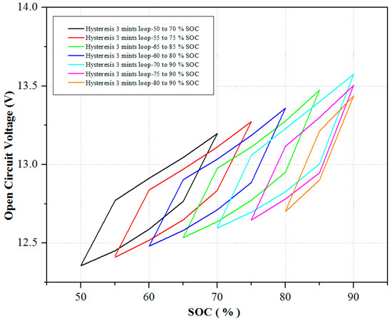
Figure 5.
Hysteresis loops (3 min) at different SOC regions.
As shown in Figure 6, the OCV follows the k1 slope for about 5 Ah charge throughput, and after that, it starts following the k2 slope. The slope is calculated by the following formula:
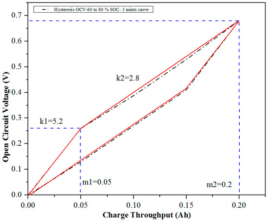
Figure 6.
Proposed hysteresis modeling.
As the rate of increase in OCV is different in different hysteresis tests, constant k1 and k2 slopes cannot be used for all the SOC regions. Whenever the hysteresis OCV starts, slopes are selected depending upon the SOC at that point, and the variation in the slopes with respect to the starting SOC is shown in Figure 7. As can be seen in Figure 7, the slopes have a linear relation with the starting SOC, which clearly means that the rate of increase in the OCV is higher in higher SOC regions and vice versa.
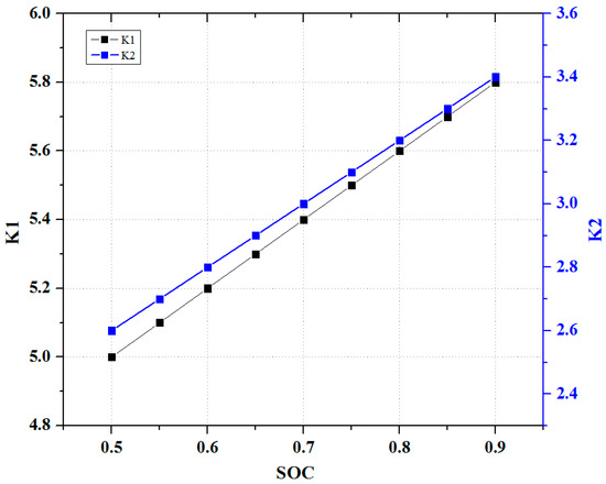
Figure 7.
Variation in hysteresis modeling slopes with respect to SOC.
Similarly, whenever a battery is discharged, hysteresis slopes are selected based on the SOC at that point. Based on the linear relationship of the slopes and starting SOC, the overall hysteresis OCV can be calculated as:
3. Unscented Kalman Filter
The Unscented Kalman Filter (UKF) offers a great improvement over all other filters for addressing the issue in SOC estimation. The UKF takes the approach of a minimal set of carefully selected sample points instead of using linearization. When these points are propagated through the actual nonlinear system, they capture the posterior mean and covariance with a high accuracy and use unscented transformation instead of solving a Jacobian matrix for non-linear systems, which makes them stabler and better in terms of performance. The more nonlinear a system is, the better the performance of the UKF. The UKF also consists of prediction, observation, and measurement stages. The discrete-time state equations for a non-linear system can be given as:
where xk represents the state parameters, f and h are non-linear system functions, uk is the input, wk is the process noise vector, vk is the measurement noise vector, and yk is the observed measurement signal.
The Adaptive UKF algorithm can be summarized as:
- Initialization:
- 2.
- Generate Sigma Points:
λ is known as a scaling factor. α determines the spread of sigma points. Its value can change between 10−4 and 1. κ is usually set to ‘0’. ‘L’ represents the number of state vectors.
- 3.
- Prediction Transformation:
Propagate the sigma points through the input function and calculate the predicted state.
Calculate the propagated covariance as:
where Qw is the covariance value of the process noise and:
β is usually equal to ‘2’ for Gaussian distributions. and are the mean and covariance weights, respectively.
- 4.
- Observation Transformation:
Propagate the sigma points though the output function and calculate the predicted measurement.
Calculate the estimated covariance as:
where Rv is the covariance value of the measurement noise.
Cross covariance is calculated as:
- 5.
- Measurement Update:
Calculate the Kalman gain as:
Update the state and covariance values as:
- 6.
- Adjustment of Qw and Rv in AUKF:
In AUKF, the process noise covariance Qw and measurement noise covariance Rv do not have a constant value like in traditional UKF; instead, they are adaptively calculated in each iteration based on the covariance matching technique [24]. The basic idea of covariance matching is to make the residuals consistent with their theoretical covariances. Fk represents the covariance approximation of the residual voltage, which can be calculated as:
where e is the residual voltage of the battery at time step j and Lq represents the window size for the covariance matching. The small window size of the covariance matching could lead the filter to diverge, whereas an adaptive filter can lose the ability of adaptation by using a large window size. Therefore, an optimal window size should be used. Based on the covariance matching technique, Qw and Rv can be updated as:
So, the adaptive UKF changes the values of Qw and Rv depending upon the residual voltage error in such a way to obtain covariance matching, which can further lead to minimizing the estimation error.
The state equations for a battery model can be shown as:
While,
Cn represents the nominal capacity of the battery. Ik and Vk are the current and voltage of the battery. OCVf represents the final Open-Circuit Voltage after considering the diffusion and hysteresis effect. The charge current is negative in the above equations. wk and vk are the process and measurement noise vectors, respectively. The overall working procedure of AUKF is shown in Figure 8.
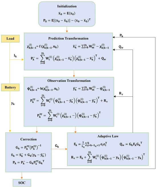
Figure 8.
Schematic diagram for Adaptive UKF.
4. Experimental Verification
For experimentation, a 90 Ah, 12 V SFLA battery from the Sebang Company, Seoul, Republic of Korea is tested for its SOC–OCV results, where it is placed in a temperature-controlled chamber at 25 degrees Celsius [25,26,27]. The OCV values were recorded during both charging and discharging phases after periods of 3 min and 3 h of rest, as illustrated in Figure 2.
4.1. Validation of Hysteresis Modeling
To verify the hysteresis modeling at different SOC regions, a special profile was created in which SOC went to a certain value, then charged up to a certain value, and then went back again. The coulomb counting method is used as a reference for the comparison of SOC estimation.
Figure 9 shows the SOC estimation results of the proposed hysteresis modeling and fixed slopes method. The simple UKF is used for estimating the SOCs of both hysteresis models, and the values of the different parameters required in UKF are given in Table 1.
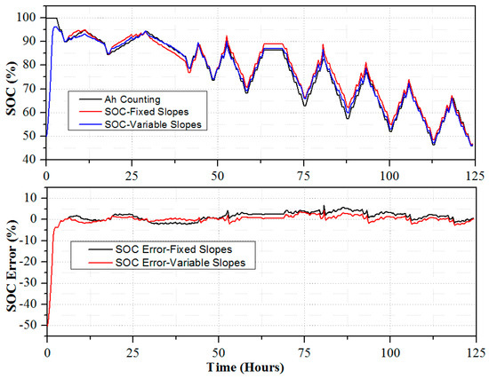
Figure 9.
Comparison of SOC estimation by proposed method.

Table 1.
Values of different parameters of UKF.
In the proposed method, the slopes always change depending on the SOC value when the battery changes its state from discharging to charging. Normally, in previous hysteresis modeling, only one hysteresis model is used for all the regions of SOC. Therefore, a comparison of the fixed slope method and the proposed method is given.
The SOC estimation results clearly show that the proposed method of hysteresis modeling is very accurate, as the error is just about 3%. When fixed slopes are used, as the hysteresis voltage increases, the SOC estimation error also starts increasing, which clearly shows that the fixed hysteresis model is not suitable for an SFLA battery. The SOC error with the fixed slope method is about 6%.
4.2. Validation of Adaptive Unscented Kalman Filter
Generally, ampere-hour counting is a simple and intuitive method that integrates the current over time, but it suffers from cumulative errors due to current sensor drift and initial SOC uncertainty. Traditional UKF is a more advanced method that uses a non-linear battery model and exploits the statistical relationships between SOC, voltage, and current. However, the UKF assumes constant values for the process and measurement noises, which may not be valid in dynamic conditions. AUKF is an improved version of UKF that adapts the noise covariances dynamically based on the voltage error in each iteration, thus enhancing the accuracy and robustness of SOC estimation.
To validate the estimation accuracy of AUKF, a random charge/discharge profile is applied on the battery with a 100% nominal capacity, as shown in Figure 10.
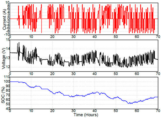
Figure 10.
Random charge/discharge profile applied on the battery.
The applied profile is designed in such a way that the SOC of the battery moves in between 100% and 50% and has both charging and discharging currents, which is more practical for finding out the estimation accuracy of the proposed algorithm.
A variable resting time is also introduced in the profile to make it more dynamic and practical. The measured terminal voltage and SOC calculated by the ampere-counting method are also shown in Figure 10.
The basic differences in both simple UKF and adaptive UKF are the values of the measurement and process noises. In simple UKF, their values are always taken as constant, while in adaptive UKF, those values are estimated based on the voltage error in each iteration, which makes AUKF more dynamic and practical in nature.
The estimation window Lq in AUKF was taken as 20 time intervals. Figure 11 shows a comparison of the simple and adaptive UKF algorithms. For simple UKF, the same parameters shown in Table 1 are used.
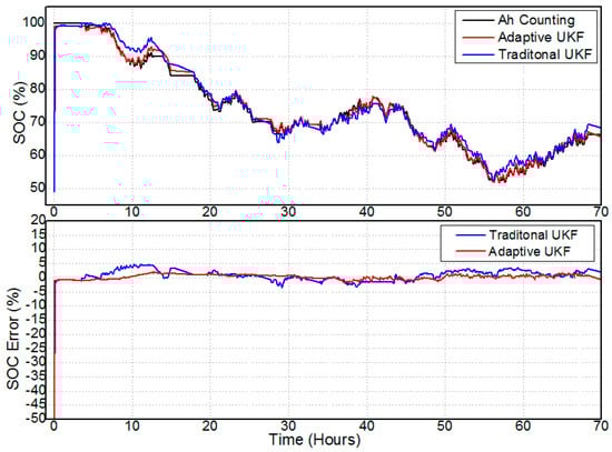
Figure 11.
Comparison of simple and adaptive UKF.
As can be observed in Figure 11 and Figure 12, adaptive UKF is fast in terms of its convergence time. It converges in about 0.07 h to the right value, while the simple UKF takes about 0.2 h.
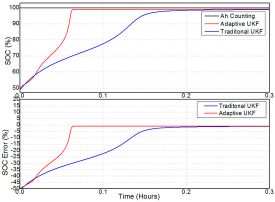
Figure 12.
SOC error of simple and adaptive UKF (Zoomed In).
In traditional UKF, the Kalman gain is, in fact, limited because of the constant values of Rv and Qw, while in AUKF, Kalman gain can freely change depending upon the residual voltage error in the battery system, which makes AUKF fast in terms of convergence time.
Similarly, after converging to the right value SOC error, AUKF does not fluctuate very fast compared to simple UKF, whose SOC error has a high fluctuation. The AUKF takes an Lq number of previous samples of residual voltage error into account for updating Rv and Qw, which makes AUKF immune to abrupt current changes happening in a battery, which can cause voltage errors for a while as well.
Traditional UKF only takes current voltage error into account and it changes the state depending upon that error, which makes the state estimated by traditional UKF more subject to fluctuation. The overall error by simple UKF is about 5%, while by using adaptive UKF, the error is reduced to about 2%. In Figure 13, the variations in the Qw and Rv are shown. Both values of these noises are updated adaptively in each iteration based on the residual voltage error.
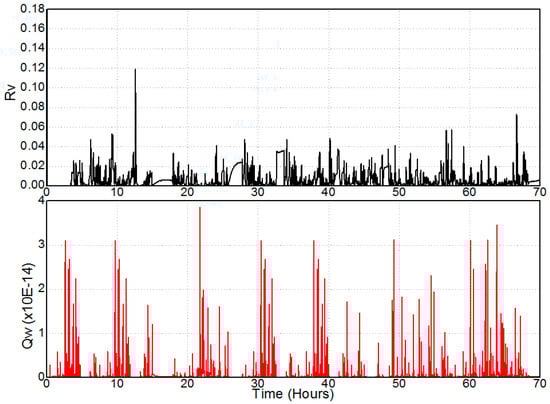
Figure 13.
Variation in Rv and Qw during the applied profile.
5. Conclusions
The Open-Circuit Voltage (OCV) behavior of an SFLA battery is investigated for the first time. Notably, our observations reveal unique hysteresis behavior distinct from other batteries, prompting the development of a novel hysteresis modeling approach. This new model is proposed and validated based on a thorough analysis of the observed hysteresis behavior. Additionally, we introduce the Adaptive Unscented Kalman Filter (AUKF) for online State of Charge (SOC) estimation in an FLA battery. AUKF stands out for its adaptive adjustment of process and measurement noise covariances. Comparisons with the traditional UKF highlight AUKF’s superior performance, demonstrated through its convergence to the correct SOC value and enhanced estimation accuracy. This emphasizes the novelty of hysteresis modeling and the advantageous performance of AUKF in SOC estimation, providing a comprehensive summary of our research findings.
Author Contributions
A.B.K. designed the algorithm of the proposed method and analyzed the algorithm of the proposed method; A.S.A. helped in preparing the final manuscript.; W.C. reviewed the manuscript and supervised the research. All authors have read and agreed to the published version of the manuscript.
Funding
This research received no external funding.
Data Availability Statement
Data are contained within the article.
Conflicts of Interest
The authors declare no conflicts of interest.
References
- Armand, M.; Tarascon, J.-M. Building better batteries. Nature 2008, 451, 652–657. [Google Scholar] [CrossRef] [PubMed]
- Huggins, R.A. Energy Storage, 1st ed.; Springer: New York, NY, USA, 2010. [Google Scholar]
- Available online: http://www.frost.com/prod/servlet/market-insight-print.pag?docid=SBRD-575K2N (accessed on 1 January 2016).
- Simatupang, D.; Benshatti, A.; Park, S.Y. Battery Internal Temperature Measurement Using LC Resonant Tank for Battery Management Systems. Batteries 2023, 9, 104. [Google Scholar] [CrossRef]
- Sheraz, M.; Choi, W. A Novel Technique for Fast Ohmic Resistance Measurement to Evaluate the Aging of Lithium-Ion xEVs Batteries. Energies 2023, 16, 1416. [Google Scholar] [CrossRef]
- Simatupang, D.; Park, S.Y. Integration of battery impedance spectroscopy with reduced number of components into battery management systems. IEEE Access 2022, 10, 114262–114271. [Google Scholar] [CrossRef]
- Duong, V.H.; Tran, N.T.; Park, Y.J.; Choi, W. Novel Estimation Technique for the State-of- Charge of the Lead-Acid Battery by using EKF Considering Diffusion and Hysteresis Phenomenon. Trans. Korean Inst. Power Electron. 2014, 19, 139–148. [Google Scholar] [CrossRef]
- Srinivasan, V.; Weidner, J.W. Hysteresis During Cycling of the Nikel Hydroxide Electrode. J. Electrochem. Soc. 2001, 148, 969–980. [Google Scholar] [CrossRef]
- Mark, V.; Edward, T. Adaptive state of charge algorithm for nickel metal hydride batteries including hysteresis phenomena. J. Power Sources 2004, 126, 236–249. [Google Scholar]
- Roscher, M.A.; Sauer, D.U. Dynamic electric behavior and open- circuit-voltage modeling of LiFePO4-based lithium-ion secondary batteries. J. Power Sources 2011, 196, 331–336. [Google Scholar] [CrossRef]
- Thele, M.; Bohlen, O.; Sauer, D.U.; Karden, E. Development of a voltage-behavior model for NiMH batteries using an impedance-based modeling concept. J. Power Sources 2008, 175, 635–643. [Google Scholar] [CrossRef]
- Windarko, N.A.; Choi, J. Hysteresis modeling for estimation of State-of-Charge in NiMH battery based on improved Takacs model. In Proceedings of the 31st International Telecommunications Energy Conference, (INTELEC), Incheon, Republic of Korea, 18–22 October 2009. [Google Scholar]
- Tang, X.; Zhang, X.; Koch, B.; Frisch, D. Modeling and estimation of nickel metal hydride battery hysteresis for SOC estimation. In Proceedings of the Prognostics and Health Management International Conference, Denver, CO, USA, 18–21 June 2008. [Google Scholar]
- Tran, N.T.; Nguyen, K.H.; Long, P.V.; Khan, A.B.; Choi, W. SOC/SOH Estimation of AGM VRLA battery by combining ARX model for online parameters estimation and DEKF considering hysteresis and diffusion effects. In Proceedings of the 9th International Conference on Power Electronics (ICPE 2015-ECCE Asia), Seoul, Republic of Korea, 1–5 June 2015; pp. 1169–1175. [Google Scholar]
- Ng, K.S.; Moo, C.S.; Chen, Y.P.; Hsieh, Y.C. An enhanced coulomb counting method for estimating state-of-charge and state-of-health of lead-acid batteries. In Proceedings of the 31st International Telecommunications Energy Conference, INTELEC 2009, Milan, Italy, 7–10 July 2009; pp. 1–5. [Google Scholar]
- Zenati, A.; Desprez, P.; Razik, H. Estimation of the SOC and the SOH of li-ion batteries, by combining impedance measurements with the fuzzy logic inference. In Proceedings of the IECON 2010—36th Annual Conference on IEEE Industrial Electronics Society, Glendale, AZ, USA, 7–10 November 2010; pp. 1773–1778. [Google Scholar]
- Shen, W.X.; Chan, C.C.; Lo, E.W.; Chau, K.T. Adaptive neuro-fuzzy modeling of battery residual capacity for electric vehicles. Ind. Electron. IEEE Trans. 2002, 49, 677–684. [Google Scholar] [CrossRef]
- Plett, G.L. Extended Kalman filtering for battery management systems of LiPB-based HEV battery packs: Part 3. State and parameter estimation. J. Power Sources 2004, 134, 277–292. [Google Scholar] [CrossRef]
- Xiong, R.; Gong, X.; Mi, C.C.; Sun, F. A robust state-of-charge estimator for multiple types of lithium-ion batteries using adaptive extended Kalman filter. J. Power Sources 2013, 243, 805–816. [Google Scholar] [CrossRef]
- Wan, E.A.; Merwe, V.D. The Unscented Kalman Filter. In Kalman Filtering and Neural Networks; Haykin, S., Ed.; John Wiley & Sons, Inc.: New York, NY, USA, 2001. [Google Scholar]
- Ge, D.; Zhang, Z.; Kong, X.; Wan, Z. Online SoC estimation of lithium-ion batteries using a new sigma points Kalman filter. Appl. Sci. 2021, 11, 11797. [Google Scholar] [CrossRef]
- Sun, F.; Hu, X.; Zou, Y.; Li, S. Adaptive unscented Kalman filtering for state of charge estimation of a lithium-ion battery for electric vehicles. Energy 2011, 36, 3531–3540. [Google Scholar] [CrossRef]
- Xia, B.; Wang, H.; Tian, Y.; Wang, M.; Sun, W.; Xu, Z. State of Charge Estimation of Lithium-Ion Batteries Using an Adaptive Cubature Kalman Filter. Energies 2015, 8, 5916–5936. [Google Scholar] [CrossRef]
- Ta, K.P.; Newman, J. Proton Intercalation Hysteresis in Charging and Discharging Nickel Hydroxide Electrodes. J. Electrochem. Soc. 1999, 146, 2769–2779. [Google Scholar] [CrossRef]
- Sheng, L.; Zhang, H.; Su, L.; Zhang, Z.; Zhang, H.; Li, K.; Ye, W. Effect analysis on thermal profile management of a cylindrical lithium-ion battery utilizing a cellular liquid cooling jacket. Energy 2021, 220, 119725. [Google Scholar] [CrossRef]
- Sheng, L.; Zhang, H.; Zhang, H.; Su, L.; Zhang, Z. Lightweight liquid cooling based thermal management to a prismatic hard-cased lithium-ion battery. Int. J. Heat. Mass. Transf. 2021, 170, 120998. [Google Scholar] [CrossRef]
- Sheng, L.; Su, L.; Zhang, H.; Li, K.; Fang, Y.; Ye, W.; Fang, Y. Numerical investigation on a lithium-ion battery thermal management utilizing a serpentine-channel liquid cooling plate exchanger. Int. J. Heat. Mass. Transf. 2019, 141, 658–668. [Google Scholar] [CrossRef]
Disclaimer/Publisher’s Note: The statements, opinions and data contained in all publications are solely those of the individual author(s) and contributor(s) and not of MDPI and/or the editor(s). MDPI and/or the editor(s) disclaim responsibility for any injury to people or property resulting from any ideas, methods, instructions or products referred to in the content. |
© 2024 by the authors. Licensee MDPI, Basel, Switzerland. This article is an open access article distributed under the terms and conditions of the Creative Commons Attribution (CC BY) license (https://creativecommons.org/licenses/by/4.0/).