Research on Coordinated Optimization of Source-Load-Storage Considering Renewable Energy and Load Similarity

Abstract

Currently, the global energy revolution in the direction of green and low-carbon technologies is flourishing. The large-scale integration of renewable energy into the grid has led to significant fluctuations in the net load of the power system. To meet the energy balance requirements of the power system, the pressure on conventional power generation units to adjust and regulate has increased. The efficient utilization of the regulation capability of controllable industrial loads and energy storage can achieve the similarity between renewable energy curves and load curves, thereby reducing the peak-to-valley difference and volatility of the net load. This approach also decreases the adjustment pressure on conventional generating units. Therefore, this paper proposes a two-stage optimization scheduling strategy considering the similarity between renewable energy and load, including energy storage and industrial load participation. The combination of the Euclidean distance, which measures the similarity between the magnitude of renewable energy–load curves, and the load tracking coefficient, which measures the similarity in curve shape, is used to measure the similarity between renewable energy and load profiles. This measurement method is introduced into the source-load-storage optimal scheduling to establish a two-stage optimization model. In the first stage, the model is set up to maximize the similarity between renewable energy and the load profile and minimize the cost of energy storage and industrial load regulation to obtain the desired load curve and new energy output curve. In the second stage, the model is set up to minimize the overall operation cost by considering the costs associated with abandoning the new energy sources and shedding loads to optimize the output of conventional generator sets. Through a case analysis, it is verified that the proposed scheduling strategy can achieve the tracking of the load curve to the new energy curve, reducing the peak-to-valley difference of the net load curve by 48.52% and the fluctuation by 67.54% compared to the original curve. These improvements effectively enhance the net load curve and reduce the difficulty in regulating conventional power generation units. Furthermore, the strategy achieves the full discard of renewable energy and reduces the system operating costs by 4.19%, effectively promoting the discard of renewable energy and reducing the system operating costs.

1. Introduction

The consumption of traditional fossil fuels has led to continuous environmental deterioration. Hence, countries around the world are actively exploring sustainable alternative energy sources to achieve sustainable development for both the economy and the environment [1,2]. As early as 2005, the Chinese government issued the Renewable Energy Law, outlining supportive policies for renewable energy, such as wind and solar power [3]. According to China’s National Energy Administration statistics, 120 million kW of new wind power generation systems was installed nationwide by the end of 2022, with power generation reaching 119 million kWh [4]. Thus, the traditional power system is transitioning toward a new energy power system, decreasing the proportion of conventional power generation units. Renewable energy on the “supply” side is gradually becoming the dominant power source. However, renewable energy exhibits significant randomness, intermittency, and uncontrollable fluctuations due to factors such as seasons and weather [5,6]. Consequently, the increasing replacement of conventional power generation units by renewable energy intensifies the demand for regulating resources in the power system while reducing its regulation capacity. This replacement poses significant challenges to the safe operation of the power system [7,8]. Hence, incorporating adjustable resources, such as controllable load-side resources and energy storage devices, into the power grid scheduling holds significant importance.

Load-side resource management, as a form of regulation, is able to realize active peaking to a certain extent and enhance the regulation capability of the power grid [9,10]. Compared to residential and commercial loads, industrial loads are characterized by a high degree of automation, a large regulation range, and low transformation costs [11]. Additionally, they have a higher willingness to participate in grid services. In [12], the response characteristics of industrial self-owned power plants and electricity load are simultaneously considered, establishing a two-level scheduling model in the interests of both the power supply company and industrial enterprises. However, it only considers the continuous adjustment characteristics of industrial enterprises, failing to fully exploit the scheduling potential. In [13], a detailed analysis of industrial electricity consumption variation patterns and operating states is provided to propose a scheduling framework that combines cascade hydropower with industrial load for smoothing out fluctuations in renewable energy output and effectively balancing the relationship between renewable energy output fluctuations and installed capacity. In [14], the behavior of different industrial users is analyzed, and a load decomposition algorithm is presented to analyze the self-scheduling process mechanism of load aggregation, establishing an optimal self-scheduling model for industrial load aggregator participation in grid scheduling. In [15], the different adjustable characteristics of industrial and residential loads are analyzed, establishing a demand response provider to coordinate the response plans of these two types of loads and improving the overall system economy by integrating the comprehensive flexibility of these two loads. In summary, current research mainly focuses on utilizing controllable industrial loads for grid scheduling. However, with the development of load-side resource scheduling technology and the improvement in various energy storage technologies, the simultaneous integration of controllable industrial loads and energy storage devices into grid scheduling is significant for optimizing scheduling solutions.

In recent years, only a few researchers have studied the coordinated scheduling of industrial load and energy storage. In [16], battery energy storage and industrial loads are discussed as the two key dispatchable means to establish a two-tier joint dispatch optimization model that takes into account the equipment configuration, planning, and operation. However, the production characteristics of industrial loads are not considered in [16]; instead, they are categorized into four types: triple-frontal, double-peak, smooth, and peak-avoidance. In [17], the characteristics of electro-magnesium loads are analyzed and incorporated into the scheduling plan. Then, the energy storage devices are configured to form a joint scheduling plan with the conventional generator sets, and an economic scheduling model is established. In [18], different regulation speeds of industrial loads and energy storage are quantified, and wind power consumption is maximized using industrial loads with slow regulation speeds in the day-ahead phase. In addition, wind power fluctuations are smoothed out using energy storage that can regulate quickly in the intraday phase, improving the source-load flexibility. In [19], the regulation of cement enterprises is treated as a discrete regulation problem and uses the energy storage system to provide continuous and fine power changes coordinated by model predictive control. The combination of the two can follow the regulation or load-tracking commands accurately and maximize the daily profit. Although the joint scheduling of industrial loads and energy storage devices has been analyzed in the literature to formulate the day-ahead scheduling plan, the associated models only have considered the economy of overall scheduling and neglected the constraints on the difference between the renewable energy curve and the load curve, i.e., the net load smoothness, leading to large fluctuations in the power output of the conventional units, frequent starting and stopping, and undesired ramping of the units.

To ensure that the load curve tracks the changes in the new energy curve, smooths the net load curve, and reduces the power fluctuation of conventional generator sets, a few researchers have studied the use of energy storage or adjustable load to smooth the net load curve. In [20], a similarity measurement index for renewable energy–load curves is established based on Euclidean distance and Dynamic Time Warping (DTW) distance to characterize the load characteristics of high-proportion new energy power systems. However, DTW distance cannot be used as a metric function. In [21], an improved Euclidean distance and DTW distance are used as metrics to measure the similarity of the new energy–load curve and introduced as constraints for the source-load-storage optimization model to smooth the net load curve. However, the established metrics perform poorly in portraying the temporal similarity of the new energy–load curves and do not take the operating characteristics of the load into account [21]. In [22], the correlation coefficient is used as a new energy–load similarity index in the source-load-storage optimization model to smooth the net load curve. However, the correlation coefficient is mainly a measure of curve shape similarity, which does not reflect the curve similarity comprehensively and does not consider the dispatch economy of controllable loads in the dispatch model.

This paper proposes a source-load-storage optimization scheduling strategy considering renewable energy and load similarity based on the problems identified in the literature. Firstly, the Euclidean distance, which measures the similarity of magnitude, and the load tracking coefficient, which measures the similarity of shape, are combined to form a comprehensive measure. Then, the obtained comprehensive measures are introduced into the source-load-storage scheduling to design a two-phase scheduling framework considering the joint participation of industrial loads and energy storage that considers renewable energy and load similarity. To maximize the smoothness of the net load curve and take into account the system’s operation cost, the first stage aims to maximize the renewable energy and load similarity and minimize the dispatch costs of energy storage and industrial load. The second stage aims at minimizing the system’s operation cost to establish a two-stage model. Finally, the multi-objective gray wolf algorithm and adaptive quadratic difference evolutionary algorithm are used to solve the model, and a few case studies are discussed to prove the model’s validity.

2. Renewable Energy and Load Similarity Measure

The more similar the new energy resources and load curves, the smoother the net load curve. The Euclidean distance is the most commonly used similarity measure among the current curve similarity measurement techniques. However, the Euclidean distance reflects the magnitude similarity of the time series and is not effective in measuring the curve shape similarity. To measure the source-load similarity when time series are used, the magnitude similarity and morphological similarity of the two curves need to be considered at the same time. The load tracking coefficient defined in [23] is able to quantitatively assess the characteristics of a power source tracking load, i.e., the source-load morphological similarity. Therefore, this paper proposes a comprehensive renewable energy and load similarity measure by combining the Euclidean distance with the load tracking coefficient.

2.1. Renewable Energy and Load Data Normalization

To remove the effect of the order of magnitudes of both source and load data on the measurement method, the data need to be normalized as follows:

$$P_{\mathit{new}}^{\prime }=\frac{P_{\mathit{new}}-\min (P_{\mathit{new}})}{\max (P_{\mathit{new}})-\min \left(P_{\mathit{new}}\right)}$$

(1)

$$P_L^{\prime }=\frac{P_L-\min (P_L)}{\max (P_L)-\min \left(P_L\right)}$$

(2)

where $P_{\mathit{new}}^{\prime }$ and $P_L^{\prime }$ are the renewable energy output and load values after normalization, respectively. In addition, $\max (P_{new})$ and $\min (P_{new})$ are the maximum and minimum values of new energy output power, respectively. Moreover, $\max (P_L)$ and $\min (P_L)$ are the maximum and minimum load power values, respectively.

2.2. Euclidean Distance

$$D_1=\sqrt{{\displaystyle \sum _{t=1}^T{\left(P_L^{\prime }\left(t\right)-{P_{new}}^{\prime }\left(t\right)\right)}^2} }$$

(3)

where $D_1$ is the Euclidean distance, $T$ represents the scheduling period, $P_L^{\prime }(t)$ indicates the normalized load value of the system at time $t$, and ${P_{new}}^{\prime }(t)$ denotes the normalized new energy output value of the system at time $t$.

2.3. Load Tracking Factor

$$D_2=\frac{1}{T-1}{\displaystyle \sum _{t=1}^{T-1}\left|{\alpha }_{new}^t-{\alpha }_L^t\right|}t=1,2,\cdots ,T-1$$

(4)

where $D_2$ is the load tracking coefficient. In addition, ${\alpha }_{new}^t$ and ${\alpha }_L^t$ are the rate of change of renewable energy output power and the rate of change of load power after normalization, respectively.

2.4. Net Load Smoothness Measure Function

$$F_1=\alpha D_1+\beta D_2$$

(5)

where $\alpha$ and $\beta$ are the weights of the Euclidean distance and load tracking factor, respectively. The smaller the net load smoothness function, the stronger the matching characteristics of new energy output and load, and the smaller the net load volatility.

3. A Two-Phase Scheduling Framework for Energy Storage and Industrial Load Participation Considering Renewable Energy and Load Similarity

The rising proportion of new energy resources increases the difficulty of system-peaking regulation. The net load fluctuations and peak-to-valley differences increase compared to the original system, which hinders the utilization of new energy resources and leads to frequent fluctuations in the output of conventional power generation. Moreover, existing studies have shown that both energy storage and controllable loads can improve the load profile and promote the utilization of new energy resources and system optimal operation [24]. Therefore, this paper proposes a two-phase scheduling framework with storage and industrial load participation considering renewable energy and load similarity, as shown in Figure 1.

The dispatching plan in the first stage takes complete advantage of the regulating capacities of an electrolytic aluminum load, cement load, and energy storage power plant to obtain the optimal load curve. The goal of the first stage is to optimize net load smoothness, minimize the regulating cost of adjustable resources, and pass it to the second-phase dispatching plan.

The second-stage scheduling plan is based on the optimized load data as well as wind and solar power data, considering the regulation cost of conventional generator sets and the cost of abandoned wind, abandoned solar, and lost load power. The aim is to find the optimal power of each unit to achieve an optimal system economy.

4. Modeling of Two-Stage Scheduling Considering Renewable Energy and Load Similarity

4.1. Phase I Scheduling Model

4.1.1. Objective Function

The first stage of the scheduling model aims to minimize the renewable energy and load similarity metric function and the regulation cost of the adjustable resources.

(1)

Objective 1: The renewable energy and load similarity metric function is given by (5).

(2)

Objective 2: The cost of adjustable resources is given by (6).

$$F_2={\displaystyle \sum }_{i=1}^{N_{\mathrm{A}}}(k_i^{\mathrm{ADR}}|P_i^{\mathrm{ADR}}{\beta }_{i,t}^{\mathrm{ADR}}|)+{\displaystyle \sum }_{i=1}^{N_{\mathrm{B}}}(k_i^{\mathrm{BDR}}{u}_{i,t}^{\mathrm{BDR}}|P_{i,t}^{\mathrm{BDR}}|)+{\displaystyle \sum }_{i=1}^{N_{\mathrm{erss}}}{k}_{\mathrm{ES}}\left|P_{i,t}^{\mathrm{erss}}\right|$$

(6)

where $P_{i,t}^{\mathrm{erss}}$ represents the power of ith energy storage power station at time t; $k_{\mathrm{ES}}$ denotes the cost of charging and discharging battery energy storage. In addition, $N_{\mathrm{A}}$ and $N_{\mathrm{B}}$ are the number of cement and aluminum enterprises, respectively. Moreover, $k_i^{\mathrm{ADR}}$ indicates the per unit power compensation price of ith cement enterprise, $P_i^{\mathrm{ADR}}$ signifies the power of each crusher of the ith cement enterprise, ${\beta }_{i,t}^{\mathrm{ADR}}$ symbolizes the number of regulating crushers of the ith cement enterprise at time t, $k_i^{\mathrm{BDR}}$ defines the per unit power compensation price of regulating load of the ith aluminum electrolysis enterprise, $P_{i,t}^{\mathrm{BDR}}$ represents the power of regulating load of the ith aluminum electrolysis enterprise at time t, and $u_{i,t}^{\mathrm{BDR}}$ denotes the running state of the ith aluminum electrolysis load at time t.

4.1.2. Optimization Constraints

(1)

Cement load constraints:

There are four main processes in a cement plant: crushing, kiln feed preparation, clinker production, and fine grinding. The most flexible process for regulation is the crushing process, which accounts for about 5% of the overall electricity consumption of a cement plant. A raw material storage depot is built between the crushing process and the kiln feed preparation stage [25]. Due to the existence of the storage depot, cement factory load can be regulated by starting and stopping the crusher, with the following constraints:

• ①

  Regulating crusher quantity constraints:

  $$\begin{array}{c}{\beta }_i^{\mathrm{Amax}-}\le {\beta }_{\underset{ }{i,t}}^{\mathrm{ADR}}\le {\beta }_i^{\mathrm{Amax}+}\end{array}$$

  (7)

  where ${\beta }_i^{\mathrm{Amax}+}$ and ${\beta }_i^{\mathrm{Amax}-}$ are the maximum and minimum number of crushers that can be selected in the ith cement company, respectively.

  ②

  Cement company storage constraints:

Since the cement load scheduling considered in this paper is the first process, the raw material storage generated by the crushing link must be constrained to avoid affecting the production of subsequent processes. In [26], the raw material storage is mapped to electricity, then the constraints for each period can be expressed as follows:

$$\left\{\begin{array}{l}{S}_{i,t+1}^{\mathrm{A}}=S_{i,t}^{\mathrm{A}}+P_i^{\mathrm{ADR}}{\beta }_{i,t}^{\mathrm{ADR}}\\ 0\le S_{i,t}^{\mathrm{A}}\le S_i^{\mathrm{Amax}}\\ S_{i,0}^{\mathrm{A}}=S_{i,T}^{\mathrm{A}}\end{array}\right.$$

(8)

where $S_{i,t}^{\mathrm{A}}$ represents the storage capacity of crushed raw materials of ith cement enterprise at time t, and $S_i^{\mathrm{Amax}}$ denotes the maximum storage capacity of crushed raw materials of ith cement enterprise.

(2)

Electrolytic aluminum load constraints:

Since a small change in the electrolyzer voltage will not destroy the thermal stability of the electrolyzation, aluminum electrolysis enterprises regulate their loads by changing the tank voltage [27]. However, the electrolytic aluminum load cannot be adjusted frequently without affecting the product quality. The relevant constraints are as follows:

• ①

  Upper and lower power constraints:

  $$P_i^{\mathrm{Bmin}}\le P_{i,t}^{\mathrm{BDR}}\le P_i^{\mathrm{Bmax}}$$

  (9)

  where $P_i^{\mathrm{Bmax}}$ and $P_i^{\mathrm{Bmin}}$ are the maximum increase and decrease values of load power of the ith electrolytic aluminum enterprise participating in the dispatch, respectively.

  ②

  Electrolytic aluminum load regulation time constraints:

  $$(u_{i,t-1}^{\mathrm{BDR}}-u_{i,t}^{\mathrm{BDR}})\left(T_{i.on,t}^{\mathrm{BDR}}-T_{i.on,min}^{\mathrm{BDR}}\right)\ge 0$$

  (10)

  where $u_{i,t}^{\mathrm{BDR}}$ represents the operating state of the ith electrolytic aluminum load at time t, $T_{i.on,min}^{\mathrm{BDR}}$ indicates the minimum continuous response time of the ith electrolytic aluminum load, and $T_{i.on,t}^{\mathrm{BDR}}$ denotes the response time of the ith electrolytic aluminum load at time t.

(3)

Electrochemical energy storage plant constraints:

①

Energy storage charge/discharge power:

$$P_{i,\mathrm{dis}\_\max }^{\mathrm{erss}}\le P_{i,t}^{\mathrm{erss}}\le P_{i,\mathrm{ch}\_\max }^{\mathrm{erss}}$$

(11)

where $P_{i,\mathrm{dis}\_\max }^{\mathrm{erss}}$ and $P_{i,\mathrm{ch}\_\max }^{\mathrm{erss}}$ are the maximum output and input powers of the ith energy storage device, respectively.

②

Energy storage state of charge:

$$P_{i,t}^{\mathrm{erss}}=\left\{\begin{array}{c}{P}_{i,t,\mathrm{dis}}^{\mathrm{erss}},P_{i,t}^{\mathrm{erss}}\ge 0\\ -P_{i,t,\mathrm{ch}}^{\mathrm{erss}},P_{i,t}^{\mathrm{erss}}<0\end{array}\right.$$

(12)

$$E_{i,t}^{\mathrm{erss}}=\left\{\begin{array}{c}\left(1-\tau \right)E_{i,t-1}^{\mathrm{erss}}+{\eta }_{\mathrm{ch}}{P}_{i,t,\mathrm{ch}}^{\mathrm{erss}}\\ \left(1-\tau \right)E_{i,t-1}^{\mathrm{erss}}+{\eta }_{\mathrm{dis}}{P}_{i,t,\mathrm{dis}}^{\mathrm{erss}}\end{array}\right.$$

(13)

$${\lambda }_{\min }{C}_i^{\mathrm{erss}}\le E_{i,t}^{\mathrm{erss}}\le {\lambda }_{\max }{C}_i^{\mathrm{erss}}$$

(14)

where $E_{i,t}^{\mathrm{erss}}$ represents the state of charge of ith energy storage device at time t, and $\tau$ denotes the loss coefficient of the storage plant. Moreover, ${\eta }_{\mathrm{ch}}$ and ${\eta }_{\mathrm{dis}}$ are the energy input and output conversion efficiency of the storage plant. $C_i^{\mathrm{erss}}$ signifies the ith energy storage device. ${\lambda }_{\max }$ and ${\lambda }_{\min }$ indicate the maximum and minimum state of charges of the storage plant, respectively.

4.2. Phase II Scheduling Model

4.2.1. Objective Function

The second phase has the minimization of system operating costs as an objective function and is given as follows:

$$\left\{\begin{array}{l}{F}_3=f_{G,t}+f_{cut,t}\\ f_{G,t}={\displaystyle \sum _{i=1}^{N_G}}[(a_i{P}_{G,i,t}^2+b_i{P}_{G,i,t}+c_i)+S_i\left(1-u_{G,i,t-1}\right)u_{G,i,t}]\\ f_{cut,t}=k^{\mathrm{Wcut}}{P}_t^{\mathrm{Wcut}}+k^{\mathrm{PVcut}}{P}_t^{\mathrm{PVcut}}+k^{\mathrm{Lcut}}{P}_t^{\mathrm{Lcut}}\end{array}\right.$$

(15)

where $f_{G,t}$ represents the cost of conventional generator sets, $f_{cut,t}$ indicates the sum of the costs associated with wind abandonment, solar abandonment, and load loss, $N_G$ denotes the number of conventional generator sets, and $P_{Gi,t}$ symbolizes the generated power from ith conventional generator set at time t. $a_i$, $b_i$, and $c_i$ are the coal consumption coefficients of ith conventional generator set, $S_i$ defines the start–stop cost coefficient of ith conventional generator set, and $u_{G,i,t}$ represents the start–stop state of ith conventional generator set at time t. $k^{\mathrm{Wcut}}$, $k^{\mathrm{PVcut}}$, and $k^{\mathrm{Lcut}}$ are the penalty prices for wind abandonment, solar abandonment, and load loss, respectively. Furthermore, $P_t^{\mathrm{Wcut}}$, $P_t^{\mathrm{PVcut}}$, and $P_t^{\mathrm{Lcut}}$ are the abandoned wind, abandoned solar, and lost load power at time t, respectively.

4.2.2. Restrictive Condition

The net load of the power system is defined as follows:

$$P_t^{\mathrm{l}\text{-}\mathrm{eq}}=P_t^{\mathrm{load}}-P_t^{\mathrm{W}}-P_t^{\mathrm{PV}}$$

(16)

where $P_t^{\mathrm{l}\text{-}\mathrm{eq}}$ is the net load of the power system, $P_t^{\mathrm{load}}$ represents the active load of the system at time t without considering the participation of controllable loads, $P_t^{\mathrm{W}}$ denotes the wind power output at time t, and $P_t^{\mathrm{PV}}$ indicates the solar power output at time t.

(1)

Power balance constraints:

$${\displaystyle \sum }_{i=1}^{N_G} P_{G,i,t}+P_{i,t}^{\mathrm{erss}}-P_t^{\mathrm{Wcut}}-P_t^{\mathrm{PVcut}}=P_t^{\mathrm{l}\text{-}\mathrm{eq}}+{\displaystyle \sum }_{i=1}^{N_{\mathrm{A}}}{P}_i^{\mathrm{ADR}}{\beta }_{i,t}^{\mathrm{ADR}}+{\displaystyle \sum }_{i=1}^{N_{\mathrm{B}}}{P}_{i,t}^{\mathrm{BDR}}-P_t^{\mathrm{Lcut}}$$

(17)

(2)

Conventional generator set constraints:

①

Upper and lower power limits for conventional generator sets:

$$u_{G,i,t}{P}_{G,i}^{\min }\le P_{G,i,t}\le u_{G,i,t}{P}_{G,i}^{\max }$$

(18)

where $P_{G,i}^{\min }$ and $P_{G,i}^{\max }$ are the maximum and minimum values of the power of the ith conventional generator set, respectively. In addition, $u_{G,i,t}$ indicates the start and stop states of the ith conventional generator set at time t, and its value 1 means start, and 0 means stop.

②

Conventional generator set climbing constraints:

$$P_{G,i,t}-P_{G,i,t-1}\le u_{i,t}{R}_i$$

(19)

$$P_{G,i,t-1}-P_{G,i,t}\le u_{i,t-1}{R}_i$$

(20)

where $R_i$ denotes the ramp rate of the ith conventional generator set.

③

Minimum start-up and shutdown times of conventional generator sets:

The conventional generator sets cannot be started and stopped frequently during operation and need to be kept in a running state for a certain period as follows:

$$(u_{G,i,t-1}^{ }-u_{G,i,t}^{ })\left(T_{i.on,t-1}^G-T_{i.on}^G\right)\ge 0$$

(21)

$$(u_{G,i,t}^{ }-u_{G,i,t-1}^{ })\left(T_{i.off,t-1}^G-T_{i.off}^G\right)\ge 0$$

(22)

where $T_{i.on}^G$ and $T_{i.off}^G$ are the continuous on-time and continuous off-time of the ith conventional generator set, respectively.

(3)

Wind abandonment, solar abandonment, and lost load constraints:

$$0\le P_t^{\mathrm{Wcut}}\le P_t^{\mathrm{Wf}}$$

(23)

$$0\le P_t^{\mathrm{PVcut}}\le P_t^{\mathrm{PVf}}$$

(24)

$$0\le P_t^{\mathrm{Lcut}}\le P_t^{\mathrm{Lf}}$$

(25)

where $P_t^{\mathrm{Wf}}$, $P_t^{\mathrm{PVf}}$, and $P_t^{\mathrm{Lf}}$ are the predicted values of wind, solar, and load power at time t, respectively.

(4)

Power constraints of transmission lines:

$$-P_{ij}^{\max }\le B_{ij}\left({\theta }_{i,t}-{\theta }_{j,t}\right)\le P_{ij}^{\max }$$

(26)

where $P_{ij}^{\max }$ represents the maximum power delivered by the transmission line between nodes i and j, $B_{ij}$ denotes the susceptance between nodes i and j, and ${\theta }_{i,t}$ indicates the phase angle at node i at time t.

5. Net Load Smoothness Evaluation Index

To show that the proposed strategy can increase the similarity between renewable energy and load, thus improving the smoothness of net load, the curve volatility and peak-to-valley difference metrics are used to evaluate and compare the net load curves quantitatively.

5.1. Indicators of the Volatility of the Curve

$$I_s=\frac{1}{T-1}{\displaystyle \sum _{t=1}^{T-1}\left|\frac{P_{\mathrm{equ}}^{t+1}-P_{\mathrm{equ}}^t}{T-1}\right|}t=1,2,\cdots ,T$$

(27)

where $P_{\mathrm{equ}}^{t+1}$ denotes the net load power at the current instant and $P_{\mathrm{equ}}^t$ indicates the net load power at the previous instant.

5.2. Indicators of Peak-to-Valley Differences in Curves

$$P_{\mathrm{m}}=P_{\max }-P_{\min }$$

(28)

where $P_{\max }$ and $P_{\min }$ are the maximum and minimum values of the curve, respectively.

6. Case Study

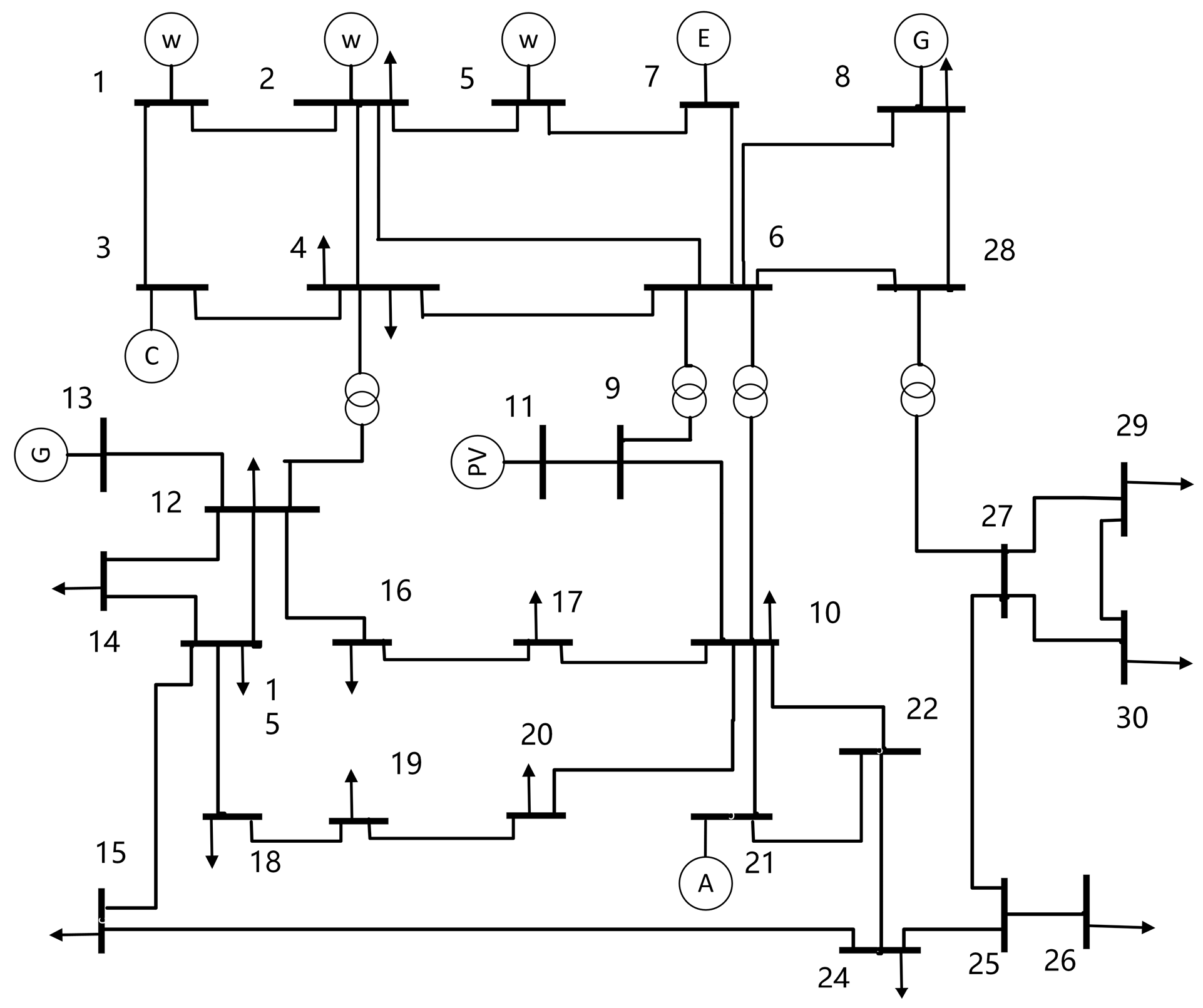
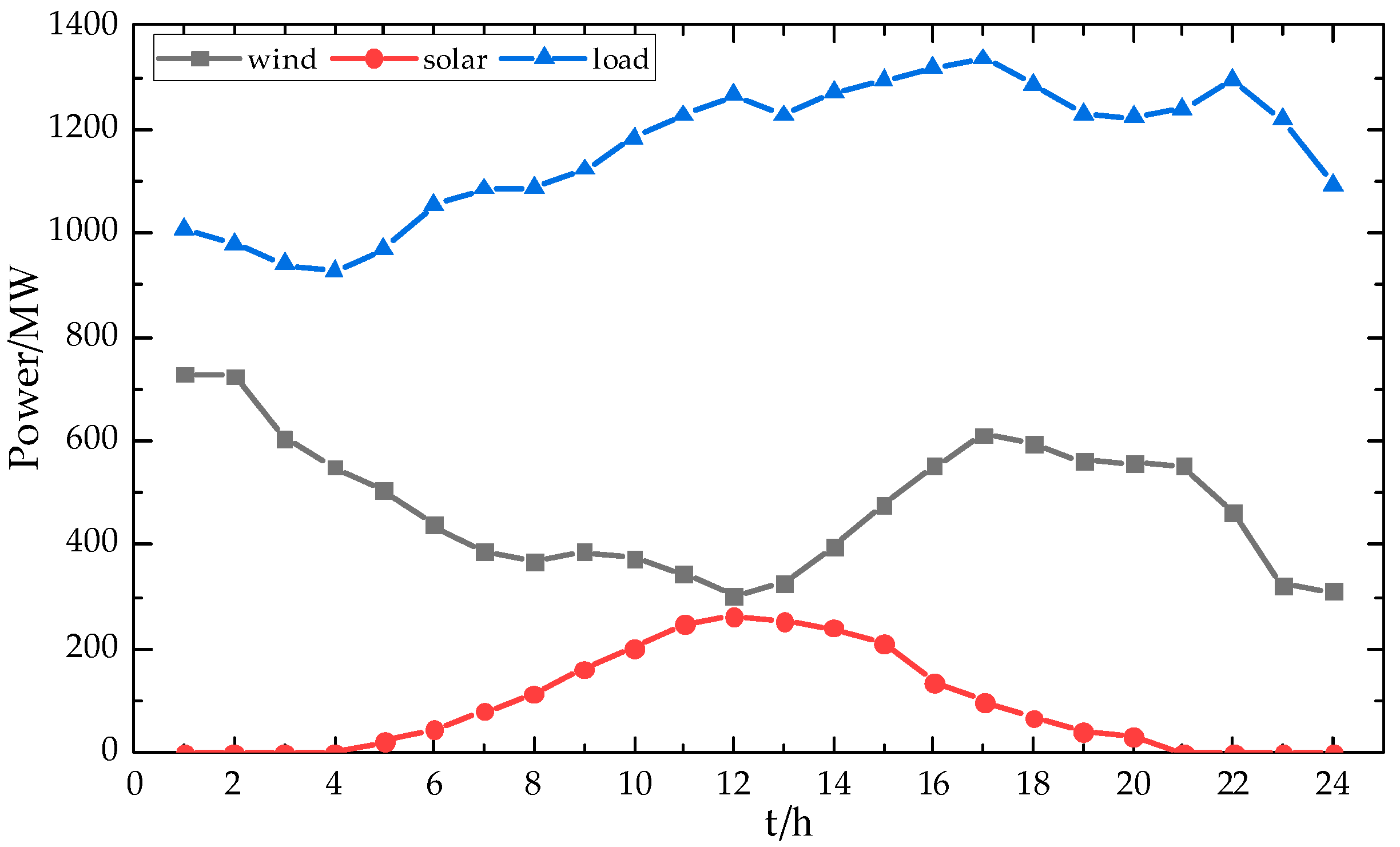
6.1. Description

The proposed two-stage optimization model is demonstrated by considering a modified IEEE30 node system as an example. Figure A1 of Appendix A shows that the improved IEEE30 node system contains two conventional generator sets and four renewable energy field stations. The parameters of the conventional generator sets are shown in

Table A1. Parameters of Conventional Generator Set.

Parameters	Rated Power/MW	Minimum Power/MW	Climb Rate Range/(MW·h−1)	Minimum Start/Stop Time/h	Start-Up Costs/CNY	Downtime Costs/CNY	Cost Factor a/b/c
Unit 1	800	250	−250~250	5\4	900,000	400,000	0.00173/20.26/244.2
Unit 2	500	150	−150~150	5\4	900,000	400,000	0.0021/24.68/176.8

of Appendix A. The renewable energy farms are connected to nodes 1, 2, 5, and 11, with a net installed capacity of 300 MW. The prediction curves of the system’s wind, solar, and load powers are shown in Figure A2 in Appendix A. The energy storage station in the system is connected to node 7, with its parameters being discussed in [17]. The cement load and aluminum electrolysis load are, respectively, connected to nodes 3 and 21, with their specific parameters shown in

Table A2. Resource parameters can be regulated.

Parameters	Cement	Parameters	Aluminum Electrolysis
Maximum number of pulverizers’ increase/decrease	13/24	Regulate the upper and lower power limits/MW	56/−45
Power per pulverizer/MW	2	Minimum continuous running time/h	2
Compensatory price in CNY/(MW·h)	60	Compensatory price in CNY/(MW·h)	60
Maximum storage capacity/(MW·h)	250	\	\
initial capacity/(MW·h)	110	\	\

of Appendix A. The penalty cost of abandoned wind power and abandoned solar power is 300 CNY/(MW·h), and the penalty cost of lost load is 8000 CNY/(MW·h). The model discussed in this paper is a two-stage scheduling model. The first stage is a multi-objective optimization problem solved using the improved multi-objective gray wolf algorithm [28]. The second stage is solved using a differential evolutionary algorithm [29], in which the improved multi-objective gray wolf algorithm solves the first stage to obtain multiple Pareto optimal solutions. In this paper, a fuzzy affiliation function is developed to evaluate the objective function, and the optimal compromise solution is selected [30]. The fuzzy affiliation function is as follows:

$${\mu }_i=\left\{\begin{array}{ll}1& f_i\ge f_{i,\max }\\ \frac{f_i-f_{i,\min }}{f_{i,\max }-f_{i,\min }}& f_{i,\min }<f_i<f_{i,\max }\\ 0& f_i\le f_{i,\min }\end{array}\right.$$

(29)

where $f_i$ is the value of the i-th objective function, and $f_{i,\max }$ and $f_{i,\min }$ are the upper and lower limits of the range of values of this objective function, respectively. In addition, ${\mu }_i$ represents the satisfaction corresponding to the i-th objective function value.

The standardized satisfaction value $\mu$ is obtained according to Equation (30), and the solution with the largest standardized satisfaction value is selected as the optimal compromise solution.

$$\mu =\frac{1}{m}{\displaystyle \sum _{i=1}^m{\mu }_i}$$

(30)

where $m$ is the number of optimization objectives in the model.

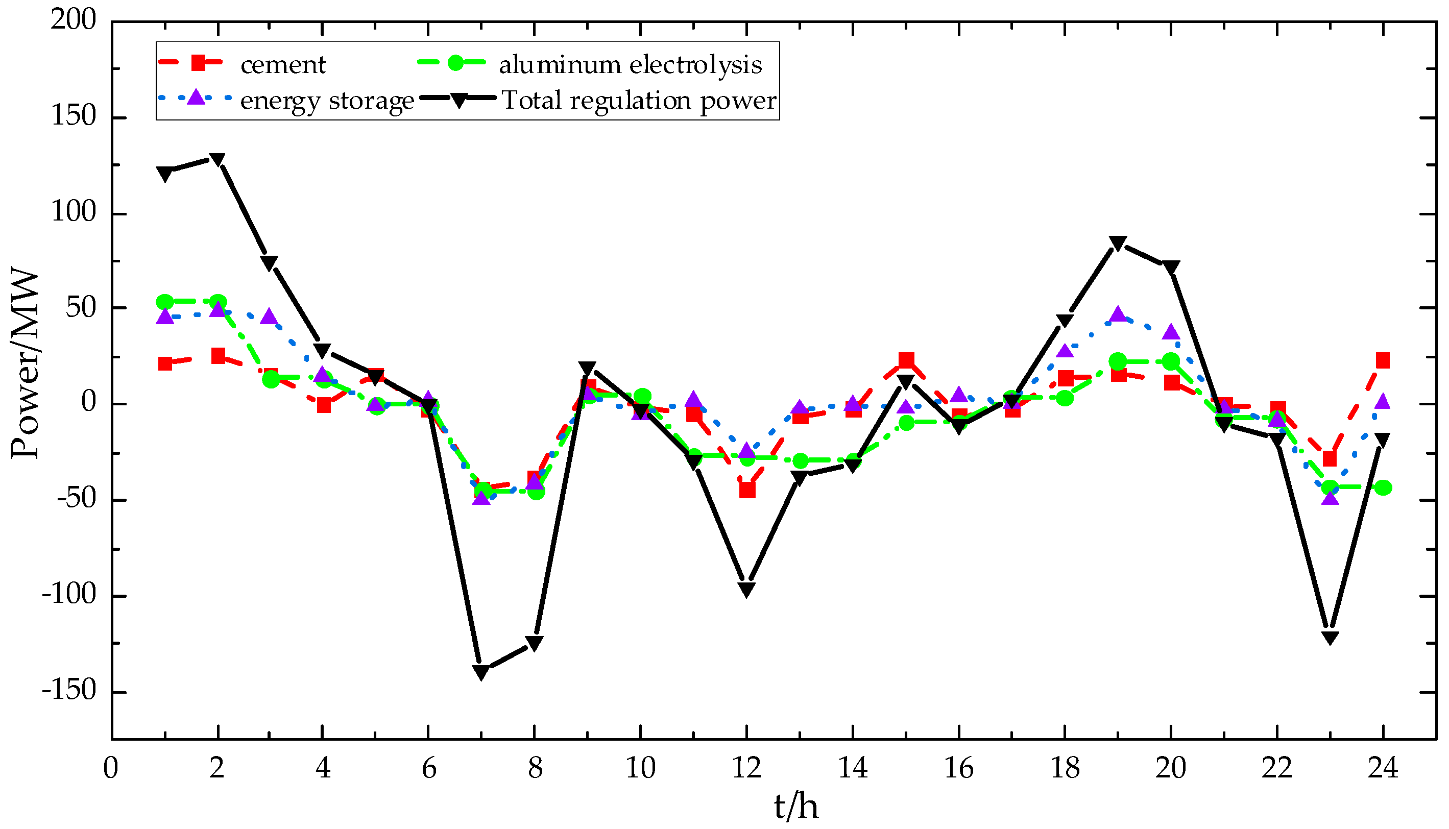
6.2. Analysis of Optimized Scheduling Results

By optimizing the first- and second-stage models, the optimized load curve and conventional unit output curve can be obtained, as shown in Figure 2. Figure 3 shows the calling plan of energy storage and industrial load. Moreover, the total regulated power in the figure is the sum of regulated powers of energy storage and industrial load.

Figure 2 and Figure 3 show that the renewable energy output is more abundant from 1:00 to 6:00 and from 17:00 to 21:00. Thus, load increase is carried out by utilizing the regulation capacity of energy storage and industrial loads during these hours. The new energy output is insufficient during 6:00–9:00 and 22:00–24:00. At 12:00, load reduction is carried out using the regulation capacity of energy storage and industrial loads during these hours. During these hours, load reduction will be carried out by utilizing energy storage and industrial load regulation capacity. Through the invocation of adjustable resources according to the scheduling strategy discussed in this paper, the optimized load curve is highly similar to the new energy output curve in terms of shape and time sequence, stabilizing the optimized net load curve. The net load power demand is supplied by the conventional units, as shown in Figure 2. The output of the optimized conventional generator set is also smoother compared to the output of the conventional generator set before optimization.

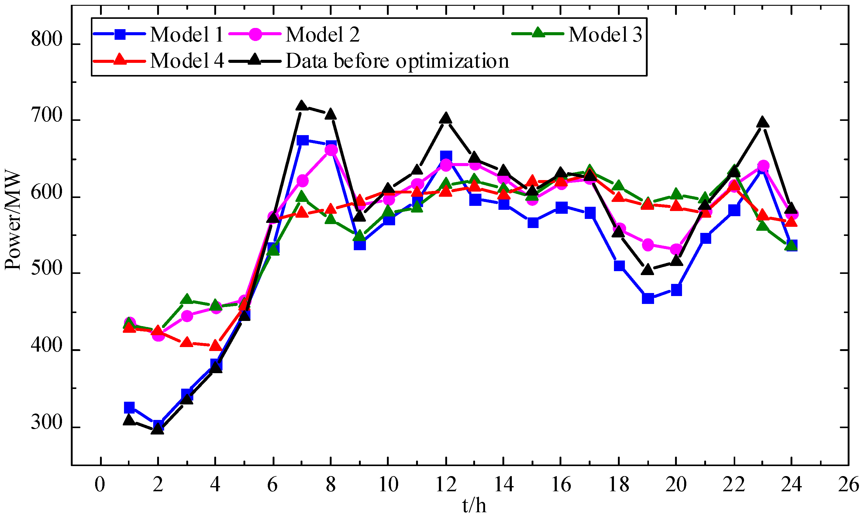
6.3. Comparative Analysis of Different Scheduling Strategies

To verify the superiority of the discussed scheduling strategy, three scenarios are selected for the analysis.

Scenario 1: A scheduling strategy that does not introduce a renewable energy and load similarity measure and does not take into account the participation of energy storage and industrial loads with the goal of economy.

Scenario 2: A scheduling strategy that does not introduce a renewable energy and load similarity measure and considers the participation of energy storage and industrial loads with the goal of economy.

Scenario 3: The scheduling strategy discussed in this paper.

The net load curves and net load smoothness index values for the three scheduling scenarios are illustrated in Figure 4 and

Table 1. Net Load Smoothness Evaluation Indicators.

Evaluation Indicators	Peak-to-Valley Difference	Volatility
Scenario 1	436	54.65
Scenario 2	312	42.67
Scenario 3	224	17.74

, respectively. As shown in Figure 4, Scenarios 1 and 2 have more intense fluctuations in the net load curve; Scenario 3 has smaller fluctuations in the net load curve and is a smoother curve. As shown in Table 1, the peak-to-valley difference and volatility of the net load profile for Scenario 3 are reduced by 212 MW and 67.54% compared to Scenario 1, respectively. A reduction of 88 MW and 58.43% in the peak-to-valley difference and volatility of the net load profile, respectively, is observed in Scenario 3 compared to Scenario 2. It can be seen that Scenario 3 effectively reduces the net load peak-to-valley difference and volatility, smoothing the net load curve.

To demonstrate the superiority of the proposed scheduling strategy, the economics of different schemes are compared, and the results are summarized in

Table 2. Costs of Different Scheduling Scenarios.

Cost Item/CNY	Conventional Generator Set	Abandonment of Renewable Energy Sources	Loss of Load	Regulatable Resources	Total Cost
Scenario 1	304,181	85,205	16	\	389,402
Scenario 2	313,251	16,897	849	44,016	375,013
Scenario 3	296,972	0	0	76,100	373,072

. As shown in Table 2, the participation of more adjustable resources in scheduling results in a remarkable reduction in the cost of abandoning renewable energy in Scenarios 2 and 3 compared to Scenario 1, leading to a reduction in the total cost of Scenarios 2 and 3. The total operating costs are comparable between Scenario 2 and Scenario 3, with an increase in adjustable resource costs but a reduction in conventional generator set operating costs and renewable energy abandonment costs. It can be seen that Scenario 3 can fully mobilize adjustable resources, promote renewable energy consumption, and decrease the total cost of system operation.

6.4. Comparative Analysis of Different Renewable Energy and Load Similarity Measures

To verify the superiority of the proposed renewable energy and load similarity measure, four scheduling models are selected for the analysis.

Model 1: The first-stage scheduling is built with a dual optimization objective of minimizing the traditional Euclidean distance and the cost of controllable load regulation.

Model 2: The first-stage scheduling is established with a dual optimization objective of minimizing the net load variance and the cost of controllable load regulation.

Model 3: The first-stage scheduling is built with a dual optimization objective of maximizing the correlation coefficient proposed in reference [22] and minimizing the cost of controllable load regulation. The formula for the correlation coefficient is as follows:

$$\left\{\begin{array}{l}R(P_{new},P_L)=\frac{\mathrm{cov}(P_{new},P_L)}{\sqrt{V_{\mathrm{var}}[P_{new}]V_{\mathrm{var}}[P_L]}}\\ \mathrm{cov}(P_{new},P_L)=\frac{{\displaystyle \sum _{t=1}^T\left[(P_{new}(t)-{\overline{P}}_{new})(P_L(t)-{\overline{P}}_L)\right]}}{T-1}\\ V_{\mathrm{var}}[P_{new}]=\frac{{\displaystyle \sum _{t=1}^T{(P_{new}(t)-{\overline{P}}_{new})}^2}}{T-1}\\ V_{\mathrm{var}}[P_L]=\frac{{\displaystyle \sum _{t=1}^T{(P_L(t)-{\overline{P}}_L)}^2}}{T-1}\end{array}\right.$$

(31)

where $\mathrm{cov}(P_{new},P_L)$ represents the covariance between new energy and load power. In addition, $V_{\mathrm{var}}[P_{new}]$ and $V_{\mathrm{var}}[P_L]$ are the variances of new energy and load power, respectively. Moreover, ${\overline{P}}_{new}$ and ${\overline{P}}_L$ indicate the average power of new energy and load power within a period.

Model 4: The first-stage scheduling is built with a dual optimization objective of minimizing the net load stability measurement function proposed in this section and the cost of controllable load regulation.

The net load curves and net load smoothness index values for the four scheduling models are illustrated in Figure 5 and

Table 3. Net Load Smoothness Evaluation Indicators.

Evaluation Indicators	Peak-to-Valley Difference	Volatility
Data before optimization	436	54.65
Model 1	373	49.70
Model 2	263	31.30
Model 3	231	24.91
Model 4	224	17.74

, respectively. As can be seen, the net load curve obtained by solving Model 1 mainly reduces the amplitude of the net load compared to the pre-optimized net load curve, leading to an insignificant decrease in the peak-to-valley difference and fluctuation of the net load. Moreover, during the 1–4 period, the net load is still lower than the minimum output of the conventional generating units (400 MW), resulting in a significant curtailment of renewable energy generation. For Model 2 and Model 3, the net load curves show a significant reduction in the peak-to-valley difference and fluctuation compared to the pre-optimized net load curve. However, there are still considerable fluctuations during the 6–8, 12, and 17–23 periods. In the 1–4 period, the net load values for both Model 2 and Model 3 are already higher than the minimum output of the conventional generating units, thus avoiding the curtailment of renewable energy generation. Model 4 exhibits the smallest peak-to-valley difference and fluctuation among the four models. The net load values are higher than the minimum output of the conventional generating units during the 1–4 period, effectively avoiding the curtailment of renewable energy generation. Compared to the original net load curve, Model 4 reduces the peak-to-valley difference and the fluctuation by 212 MW and 67.54%, respectively, demonstrating that the proposed similarity measurement method between renewable energy and load can better track the fluctuations of the optimized load curve with renewable energy, which makes the net load curve smoother and effectively reduces the curtailment of renewable energy generation, thereby alleviating the adjustment pressure on conventional generating units.

7. Conclusions

This paper proposed a two-stage optimal scheduling strategy considering renewable energy and load similarity with the participation of energy storage and industrial loads. First, a renewable energy and load similarity measure was proposed, considering both curve magnitude similarity and shape similarity. Then, energy storage and industrial loads were included in the scheduling plan. Finally, a two-stage scheduling model was established. The effectiveness of the proposed scheduling strategy was discussed in a few case studies.

(1)

Compared to traditional methods such as the Euclidean distance, net load variance, and correlation coefficient, the proposed similarity measurement method for renewable energy load can more effectively depict the matching degree of load to the output of renewable energy. Using the renewable energy and load similarity measure function to establish the adjustable resource response target can effectively reduce the peak-to-valley difference of the net load and smooth out the net load curve to stabilize the output of the conventional unit.

(2)

The two-stage scheduling model of source-load-storage coordination and optimization built in this paper aims to maximize the renewable energy and load similarity and minimize the regulation cost of adjustable resources in the upper layer and the overall operation cost in the lower layer. From an economic perspective, it can significantly reduce the cost of curtailed renewable energy and lower the overall operating cost of the system by 4.19%, thereby enhancing the overall economic efficiency of the system. From the peak regulation effect perspective, the net load peak–valley difference is reduced by 212 MW due to the participation of industrial load and energy storage in system dispatching. Moreover, the net load fluctuation is reduced by 67.54%, effectively alleviating the peak regulation pressure on conventional units and improving the level of renewable energy consumption.

It should be noted that this paper considered the industrial load involved in scheduling, including cement load and electrolytic aluminum load. However, for the cement load, only its crushing process was taken into account, and other production processes were not considered. Further research will continue to explore how to involve other production processes of cement load in system scheduling.

References

- Islam, F.; Moni, N.; Akhter, S. Feasibility Analysis of a 100MW Photovoltaic Solar Power Plant at Rajshahi, Bangladesh Using RETScreen Software. Int. J. Eng. Manuf. 2023, 13, 1–10. [Google Scholar] [CrossRef]
- Islam, M.d.S.; Islam, F.; Habib, M.d.A. Feasibility Analysis and Simulation of the Solar Photovoltaic Rooftop System Using PVsyst Software. Int. J. Educ. Manag. Eng. 2022, 12, 21–32. [Google Scholar] [CrossRef]
- Chen, W.; Zhang, Y.; Chen, J.; Xu, B. Pricing Mechanism and Trading Strategy Optimization for Microgrid Cluster Based on CVaR Theory. Electronics 2023, 12, 4327. [Google Scholar] [CrossRef]
- National Energy Board 2023 Q1 Press Conference Transcript—National Energy Board. Available online: http://www.nea.gov.cn/2023-02/13/c_1310697149.htm (accessed on 26 April 2023).
- Liu, S.; Yang, Y.; Yang, Z.; Chen, Q. Determination of Reserve Capacity Considering Random Characteristics of New Energy and Its Cost Allocation. Autom. Electr. Power Syst. 2023, 47, 10–18. [Google Scholar]
- Hu, J.; Ma, R.; Qin, K.; Liu, W.; Li, W.; Deng, H. A Demand Side Response Optimization Model Considering the Output Characteristics of New Energy. In Proceedings of the 2023 6th International Conference on Energy, Electrical and Power Engineering (CEEPE), Guangzhou, China, 12–14 May 2023; pp. 1412–1417. [Google Scholar]
- Yang, W.; Zhu, X.; Nie, F.; Jiao, H.; Xiao, Q.; Yang, Z. Chaos Moth Flame Algorithm for Multi-Objective Dynamic Economic Dispatch Integrating with Plug-In Electric Vehicles. Electronics 2023, 12, 2742. [Google Scholar] [CrossRef]
- Zhang, Z.; Zhao, Y.; Bo, W.; Wang, D.; Zhang, D.; Shi, J. Optimal Scheduling of Virtual Power Plant Considering Revenue Risk with High-Proportion Renewable Energy Penetration. Electronics 2023, 12, 4387. [Google Scholar] [CrossRef]
- Wynn, S.L.L.; Boonraksa, T.; Boonraksa, P.; Pinthurat, W.; Marungsri, B. Decentralized Energy Management System in Microgrid Considering Uncertainty and Demand Response. Electronics 2023, 12, 237. [Google Scholar] [CrossRef]
- Li, Y.; Li, R.; Shi, L.; Wu, F.; Zhou, J.; Liu, J.; Lin, K. Adjustable Capability Evaluation of Integrated Energy Systems Considering Demand Response and Economic Constraints. Energies 2023, 16, 8048. [Google Scholar] [CrossRef]
- Chang, G.; Yang, X.; Jiang, H.; Cui, Y.; Zhang, Y.; Hao, S.; Zhang, Y. Rolling flexible regulation strategy for multi-stage demand response of power grid with high proportion of new energy access considering industrial load characteristics. Electr. Power Autom. Equip. 2023, 43, 1–14. [Google Scholar] [CrossRef]
- Shu, J.; Guan, R.; Han, B. Industrial large customer time-of-use electricity price optimization method. Proc. CSEE 2018, 33, 1552–1559. [Google Scholar] [CrossRef]
- Yu, Q.; Yang, H.; Liu, J.; Liao, S.; Meng, K. Optimal allocation of wind and solar capacity based on the active response capability of cascaded hydropower and high-load energy demand power variations. Power Syst. Autom. Equip. 2020, 40, 71–78. [Google Scholar] [CrossRef]
- Oskouei, M.Z.; Zeinal-Kheiri, S.; Mohammadi-Ivatloo, B.; Abapour, M.; Mehrjerdi, H. Optimal Scheduling of Demand Response Aggregators in Industrial Parks Based on Load Disaggregation Algorithm. IEEE Syst. J. 2022, 16, 945–953. [Google Scholar] [CrossRef]
- Golmohamadi, H.; Keypour, R.; Bak-Jensen, B.; Pillai, J.R. A Multi-Agent Based Optimization of Residential and Industrial Demand Response Aggregators. Int. J. Electr. Power Energy Syst. 2019, 107, 472–485. [Google Scholar] [CrossRef]
- Hu, X.; Xu, G.; Shang, C.; Wang, L.; Weng, W.; Cheng, H. Joint planning of Battery Energy Storage and Demand Response for industrial park participating in Peak Shaving. Autom. Electr. Power Syst. 2019, 43, 116–123. [Google Scholar]
- Liu, C.; Sun, A.; Wang, Y.; He, H.; Zhang, H.; Ning, L. Day-ahead and intra-day joint economic dispatching method of electric power system considering combined peak-shaving of fused magnesium load and energy storage. Electr. Power Autom. Equip. 2022, 42, 8–15. [Google Scholar] [CrossRef]
- Hao, C.; Wang, Y.; Liu, C.; Zhang, G.; Yu, H.; Wang, D.; Shang, J. Research on Two-Stage Regulation Method for Source–Load Flexibility Transformation in Power Systems. Sustainability 2023, 15, 13918. [Google Scholar] [CrossRef]
- Xu, J.; Chen, Y.; Liao, S.; Sun, Y.; Yao, L.; Fu, H.; Jiang, X.; Ke, D.; Li, X.; Yang, J.; et al. Demand Side Industrial Load Control for Local Utilization of Wind Power in Isolated Grids. Appl. Energy 2019, 243, 47–56. [Google Scholar] [CrossRef]
- Shi, L.; Zhou, R.; Li, J.; Wang, Y.; Xu, F.; Wang, Y. New energy-load characteristic index based on time series similarity measurement. Power Syst. Autom. Equip. 2019, 39, 75–81. [Google Scholar] [CrossRef]
- Zhou, R.; Li, B.; Huang, Q.; Tang, X.; Peng, Y.; Fang, S.; Shi, L. Source-Load-Storage Coordinated Optimization Model with Source-Load Similarity and Curve Volatility Constraints. Proc. CSEE 2020, 40, 4092–4102. [Google Scholar] [CrossRef]
- Wang, T.; Li, F.; Zhou, Y.; Cui, W. Source-load-energy storage coordinated optimal scheduling for peak regulation based on new energy resource-load similarity. Electr. Power Autom. Equip. 2023, 1–10. [Google Scholar] [CrossRef]
- Ye, L.; Qu, X.; Mo, Y.; Zhang, J.; Wang, Y.; Huang, Y.; Wang, W. Analysis on intraday operation characteristics of hybrid wind-solar-hydro power generation system. Autom. Electr. Power Syst. 2018, 42, 158–164. [Google Scholar]
- Sun, C. Multiple Load Coordination Optimization Scheduling Strategy of Active Distribution Network to Improve New Energy Consumption Capacity. Master’s Thesis, North China Electric Power University, Beijing, China, 2022. [Google Scholar]
- Vujanic, R.; Mariéthoz, S.; Goulart, P.; Morari, M. Robust Integer Optimization and Scheduling Problems for Large Electricity Consumers. In Proceedings of the 2012 American Control Conference (ACC), San Diego, CA, USA, 27–29 June 2012; pp. 3108–3113. [Google Scholar]
- Golmohamadi, H.; Keypour, R.; Bak-Jensen, B.; Pillai, J.R.; Khooban, M.H. Robust Self-Scheduling of Operational Processes for Industrial Demand Response Aggregators. IEEE Trans. Ind. Electron. 2020, 67, 1387–1395. [Google Scholar] [CrossRef]
- Jin, H.; Sun, H.; Guo, Q.; Wang, B.; Cheng, R.; Wang, W. Dispatch Strategy Based on Energy Internet Customer-Centered Concept for Energy Intensive Enterprise and Renewable Generation to Improve Renewable Integration. Power Syst. Technol. 2016, 40, 139–145. [Google Scholar] [CrossRef]
- Qi, Y.; Shang, X.; Nie, J.; Huo, X.; Wu, B.; Su, W. Optimization of CCHP micro-grid operation based on improved multi-objective grey wolf algorithm. Electr. Meas. Instrum. 2022, 59, 12–19+52. [Google Scholar] [CrossRef]
- Feleke, S.; Pydi, B.; Satish, R.; Kotb, H.; Alenezi, M.; Shouran, M. Frequency Stability Enhancement Using Differential-Evolution- and Genetic-Algorithm-Optimized Intelligent Controllers in Multiple Virtual Synchronous Machine Systems. Sustainability 2023, 15, 13892. [Google Scholar] [CrossRef]
- Kannan, S.; Baskar, S.; McCalley, J.D.; Murugan, P. Application of NSGA-II Algorithm to Generation Expansion Planning. IEEE Trans. Power Syst. 2009, 24, 454–461. [Google Scholar] [CrossRef]