Abstract
To enhance the economic viability of wind energy in cold regions and ensure the safe operational management of wind farms, this paper proposes a short-term wind turbine blade icing wind power prediction method that combines principal component analysis (PCA) and fractional Lévy stable motion (fLsm). By applying supervisory control and data acquisition (SCADA) data from wind turbines experiencing icing in a mountainous area of Yunnan Province, China, the model comprehensively considers long-range dependence (LRD) and self-similar features. Adopting a combined pattern of previous-day predictions and actual measurement data, the model predicts the power under near-icing conditions, thereby enhancing the credibility and accuracy of icing forecasts. After validation and comparison with other prediction models (fBm, CNN-Attention-GRU, XGBoost), the model demonstrates a remarkable advantage in accuracy, achieving an accuracy rate and F1 score of 96.86% and 97.13%, respectively. This study proves the feasibility and wide applicability of the proposed model, providing robust data support for reducing wind turbine efficiency losses and minimizing operational risks.
1. Introduction
In recent years, with the rapid development of the global wind energy industry, wind power, as a crucial component of renewable energy, has presented broad prospects [1]. Faced with the significant challenge posed to wind energy growth by icing incidents on wind turbine blades, the accurate identification of blade icing and wind power prediction are effective measures [2,3]. Therefore, precision in feature extraction and prediction model construction is of utmost importance and has garnered significant attention from researchers. Early and accurate prediction of icing conditions is vital for operators, facilitating the timely implementation of appropriate measures to mitigate the adverse impacts of icing, enhance power generation efficiency, and reduce maintenance costs, thereby ensuring the stable operation of wind turbines [4,5].
Regarding feature extraction, Xiao et al. employed the chi-square test to rank 26 features in SCADA data and recursively eliminated low-importance features to obtain an optimal feature set [6]. Li, N et al. utilized the dynamic principal component analysis method for feature extraction and ultimately selected the yaw angle, nacelle temperature, and generator speed as relevant variables for blade icing detection [7]. Jiang, G et al. analyzed statistical characteristics and trends in continuous period ice data to construct a severity index for blade icing while selecting wind direction, ambient temperature, pitch angle, power, and wind speed as relevant features [8].
In terms of model construction, deep learning techniques have been widely applied in the field of wind turbine blade icing prediction [9,10,11]. Tao et al. addressed the issue of class imbalance in icing data by utilizing random undersampling and developed a Stacked-XGBoost blade icing diagnostic model [12]. Zhang Danfeng et al. constructed a normal behavior model based on output power and rotor speed using the XGBoost algorithm, achieving an error rate as low as 0.53% [13]. Chen et al. proposed a transfer learning TrAdaBoost algorithm model that improves performance in handling imbalanced and dynamically changing distributions of wind turbine data [14]. Tao et al., on the other hand, introduced a general model based on DNN (CNN-Attention-GRU) that combines bidirectional gated recurrent units to accurately predict wind turbine icing conditions [15,16]. The CM technique proposed by Zhang et al. employs KNN regression and a bagging ensemble strategy, resulting in approximately 30% improvement in both accuracy and operational efficiency when tested with SCADA data collected from the field [17]. In 2023, M.K. et al. proposed the BIKICE model, which utilizes time-series data and employs 5-fold cross-validation methods to conduct ice detection on wind turbine rotor blades. This approach significantly improves accuracy [18]. Xu et al. conducted an analysis of the environmental meteorological conditions, wind turbine operations, and power supply situations in a wind farm through field observations and numerical model predictions. Their findings indicate a 10.4% improvement in power forecasting compared to the original wind farm predictions [19].
To address these aforementioned issues, this paper proposes a short-term power prediction method for wind turbine blade icing based on principal component analysis (PCA) feature extraction and fractional Lévy stable motion models to tackle long-range dependence problems during the icing process of wind turbines.
The main contributions of this paper are as follows: firstly, PCA is applied to handle high-dimensional data for dimensionality reduction and feature selection, effectively addressing the issue of imbalanced data in icing prediction tasks where research on long-range dependent (LRD) features for stochastic sequences remains relatively limited [20]. Therefore, we introduce fractional Lévy stable motion models [21], which consider the influence of past and current states on future states and can better predict a series of non-smooth random processes while extracting potential icing.
2. Principal Component Analysis (PCA) Data Preprocessing
The PCA method integrates multiple health indicators to select the principal components of each feature sequence, taking into account various factors that influence the wind turbine icing process comprehensively [22]. In this preprocessing step, it is crucial to ensure that the trends in each stage are accurately reflected in the feature sequences and eliminate any redundant features [23,24]. The specific calculation steps are as follows:
Step 1: Utilize multiple feature parameter sequences as input samples for the PCA method to construct a fusion matrix.
Among them, introduces the variational mode decomposition (VMD) method, which is based on decomposed feature sequences of various health indicators [25].
Step 2: Calculate the mean value of the input sequence samples.
Step 3: Compute the correlation coefficients of sample input sequences.
where and are the rank sequences of and , respectively. If , there is a strong positive correlation between the icing feature sequence and the capacity; otherwise, there is a negative correlation.
Step 4: Calculate the eigenvalues and eigenvectors of the covariance matrix.
Step 5: Arrange the eigenvalues in descending order and select the top column eigenvectors as principal components according to the established rule, resulting in the final feature sequence [26].
3. Model Principles
3.1. Characteristics and Parameter Meanings of Lévy Stable Motion
Due to the generalized central limit theorem, there is no closed-form expression for the probability density function (PDF) of the Lévy stable distribution. Therefore, the properties of the Lévy stable distribution are represented through its characteristic function, as defined by [27].
The random process is utilized to represent a random variable that conforms to the Lévy stable distribution with the parameters . The shape of the distribution is typically influenced by and while the linear transformation of the distribution is determined by and [28].
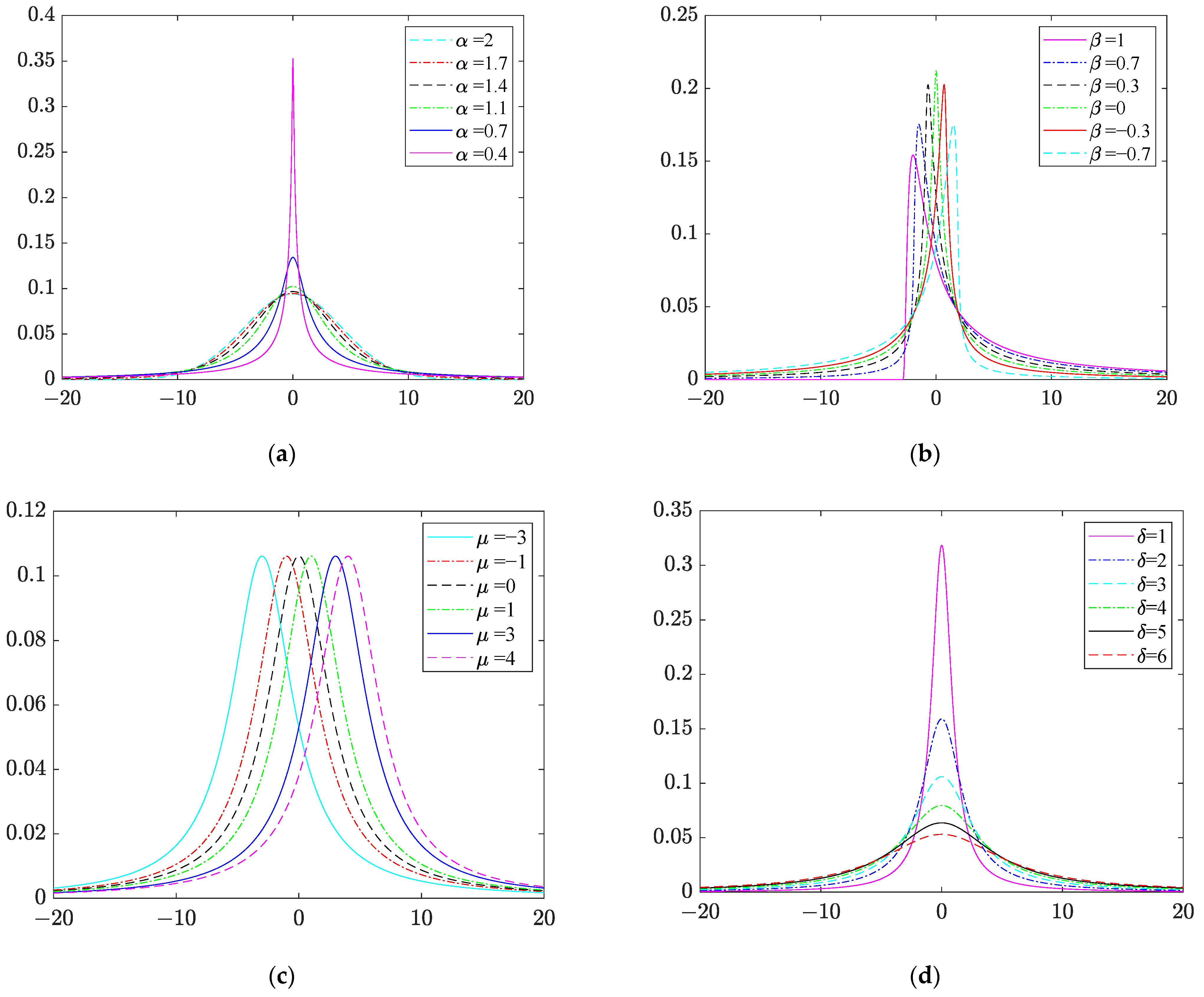
As shown in Figure 1a, the parameter represents the stability index, also known as the characteristic index. Its range is , where a larger value leads to a shorter tail and a faster decay in the distribution, while a smaller results in a greater impulsiveness in the sequence, causing larger impacts from anomalies occurring further away from the central position [29]. In (b), parameter represents the skewness parameter, with a range of [−1, 1]. When , the distribution is skewed to the left; conversely, when , the distribution is skewed to the right. When , the Lévy stable distribution is referred to as a symmetric Lévy stable distribution. In (c), the drift coefficient primarily controls the distribution’s position, representing the mean or median of the sequence. In (d), the diffusion parameter indicates the degree of deviation of the distribution from the mean. When , it represents the extent of distribution deviation from the mean and is equivalent to the variance of a normal distribution in special cases [30].
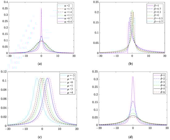
Figure 1.
Probability density distribution of different characteristic functions. (a) Different stability indexes ; (b) different skewness parameters ; (c) different drift coefficients ; (d) different diffusion coefficients .
Therefore, if the stochastic process exhibits power-law decay in its probability distribution, demonstrating heavy-tailed characteristics, it possesses long-range dependence (LRD) characteristics in the domain of autocorrelation functions [31].
3.2. fLsm Model and LRD Related Characteristics
Expression (6) for the fLsm model is given as follows:
The equation holds, where and are real constants satisfying , and represents a Lévy stable measure [32] within the Lebesgue measure space.
The LRD characteristics of the fLsm model are determined by the interplay between the self-similarity parameters and . When , the integral kernel function exhibits a slow variation with respect to variable , resulting in its divergence at infinity. This persistent effect endows the fLsm model with its distinctive LRD characteristics. The magnitude of and product directly influences the strength of LRD features in the fLsm model, leading to a more intricate and diverse developmental pattern in random sequences.
Equation (7) provides the mathematical representation of the numerical simulation sequence for the generated fLsm model:
Among them, represents Lévy stable white noise, exhibiting long-range dependence (LRD) characteristics. Figure 2 illustrates the simulation of the fLsm model under various conditions.
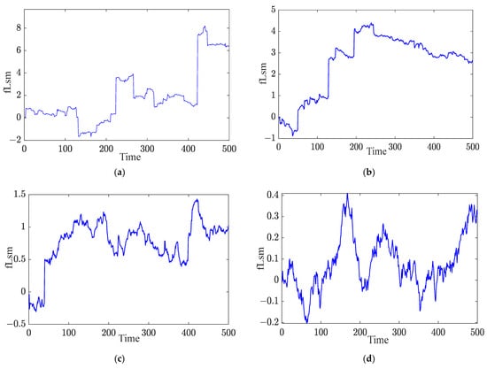
Figure 2.
Simulation sequences of the fLsm model under different conditions (a) H = 0.85, ; (b) H = 0.85, ; (c) H = 0.85, ; (d) H = 0.85, . Time representation in the figure is specified as time steps, where each time step represents the simulated sequence count.
When , as the value of increases in the fLsm model, the randomness of the sequence fluctuates more quickly or slowly, indicating a weakening of heavy-tailed peak impulses and a more prominent LRD characteristic.
4. Prediction Model Construction
4.1. Establishment of the Iterative Difference Prediction Model
The general form of the fLsm model driving the Itô process for a random sequence is given as follows [33] (Equation (8)):
In order to establish the iterative difference form of the predictive model and compute the estimated values of model parameters, we discretize the increment of the fLsm model. The discretization process adheres to Maruyama’s formula [34] and results in Equations (9) and (10):
Equation (11) is derived by substituting the fractional Lévy white noise [35] for into the aforementioned equation, thereby obtaining the increment Itô integral form of the fLsm model.
Therefore, the incremental representation of the fLsm model is expressed in a differential discrete form as [36] (Equation (12)).
The discrete form of the fractional-order Itô process is given by Equation (13).
By integrating the discrete form of a fractional-order Ito process with a distinction equation, we can derive an iterative difference prediction model based on the fLsm model (Equation (14)).
4.2. Establishment of the Iterative Difference Prediction Model
Combining the Lyapunov coefficient from chaos theory [37], we determine the maximum prediction step length of the ice formation characteristic sequence to achieve accurate forecasting of ice trends. The Lyapunov coefficient reflects the sensitivity of the ice formation characteristic sequence to initial values, which gradually increases over time. Even slight disturbances in initial values will be exponentially amplified, significantly impacting future trend changes. By calculating the maximum Lyapunov coefficient using a widely applied method for small data sets, we can determine the maximum predictable range of trends. The calculation process is as follows:
Step 1: Define the time series and determine the lag time using the autocorrelation function method.
Step 2: Employ Cao’s algorithm [38] to ascertain the appropriate embedding dimension .
Step 3: Reconstruct the phase space.
where .
Step 3: Calculate the maximum Lyapunov coefficient utilizing small-scale data analysis techniques.
where , and is the distance between each reference point and its adjacent point after the -th discrete time step:
The maximum prediction range for the ice formation feature sequence is expressed as follows:
The maximum predictive range of ice formation feature sequences can be determined by following the aforementioned steps, thereby optimizing the prediction process for icing trends.
4.3. Parameter Estimation of New Feature Functions
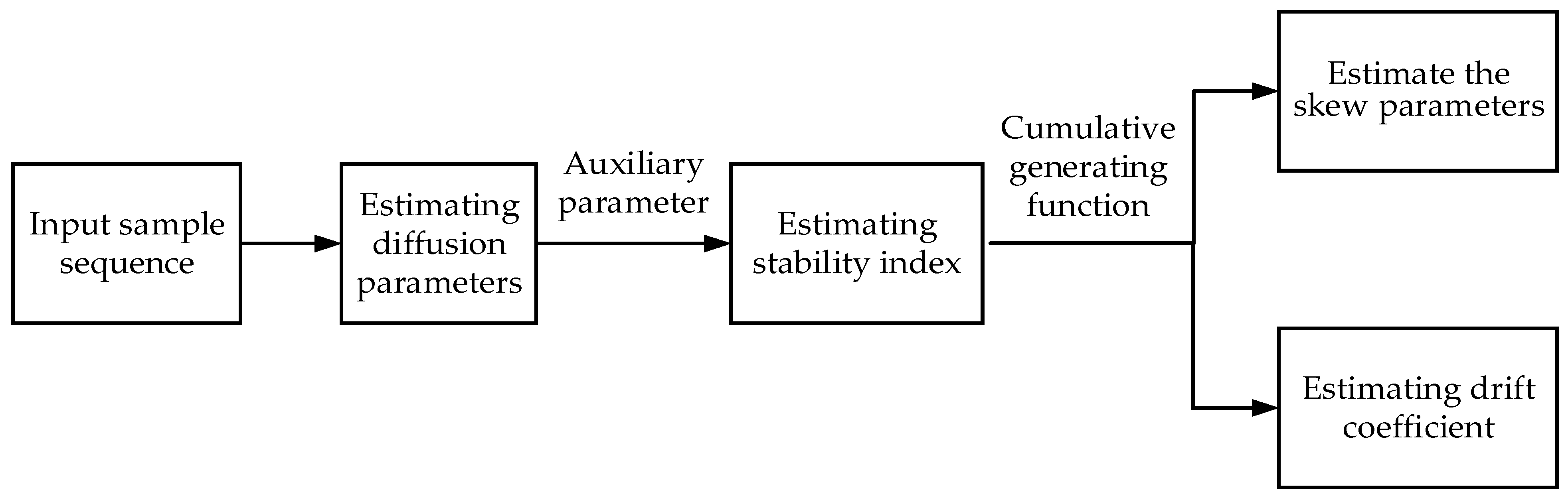
The accurate estimation of the stability index , skewness index , drift coefficient , and diffusion parameter is crucial for modeling prediction models based on fLsm. The new feature function estimation method performs parameter estimation through the following steps, as illustrated in Figure 3.
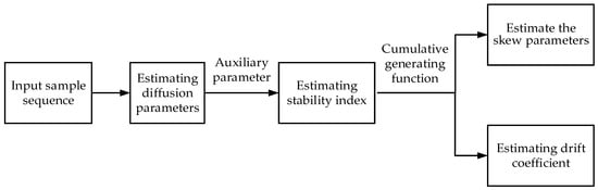
Figure 3.
Flowchart of the new feature function method.
4.3.1. Estimation of Diffusion Parameter
First, estimate the diffusion parameter for the sample sequence . Since the characteristic function is a complex function related to , the characteristic function is given by:
At the position where , the estimated value of diffusion parameter is:
4.3.2. Estimation of Stability Index
The stability index determines the correlation of the fLsm model, and different values can be used to construct various prediction models. By employing the new feature function method and combining Cauchy feature function corresponding to and Gaussian feature function corresponding to , we calculate the auxiliary parameter .
Therefore, the estimated value of the stability index α is expressed as:
4.3.3. Estimation of Skewness Index and Drift Coefficient
Equation (23) is primarily obtained by computing the logarithmic form of the feature function.
At , the real and imaginary parts are, respectively, represented as follows:
By following the above steps, estimates for the stability index , skewness index , drift coefficient , and diffusion parameter can be obtained.
5. Experimental Cases and Analysis
5.1. Data Description
To validate the performance of the proposed short-term prediction model for wind turbine blade icing in this paper, we utilized SCADA data from a wind farm in a mountainous area in Yunnan province, China. The dataset includes monitoring data from five doubly fed asynchronous wind turbine generators, spanning from 24 January 2018 to 31 December 2018, with a time resolution of 4 min. The dataset consists of 19 original feature variables, and the parameters are explained in Table 1.

Table 1.
Explanation of the 19 feature variable parameters in the dataset.
Each sample is labeled with a status tag, where icing state data are labeled as ‘0’ and normal state data are labeled as ‘1’. Since the wind turbine icing events occurred only from 19:00 on 29 December 2018 to 24:00 on 31 December 2018, the data quantities and ratios for the five turbine units are presented in Table 2.
Table 2.
Statistical parameters of the dataset.
5.2. Experimental Process
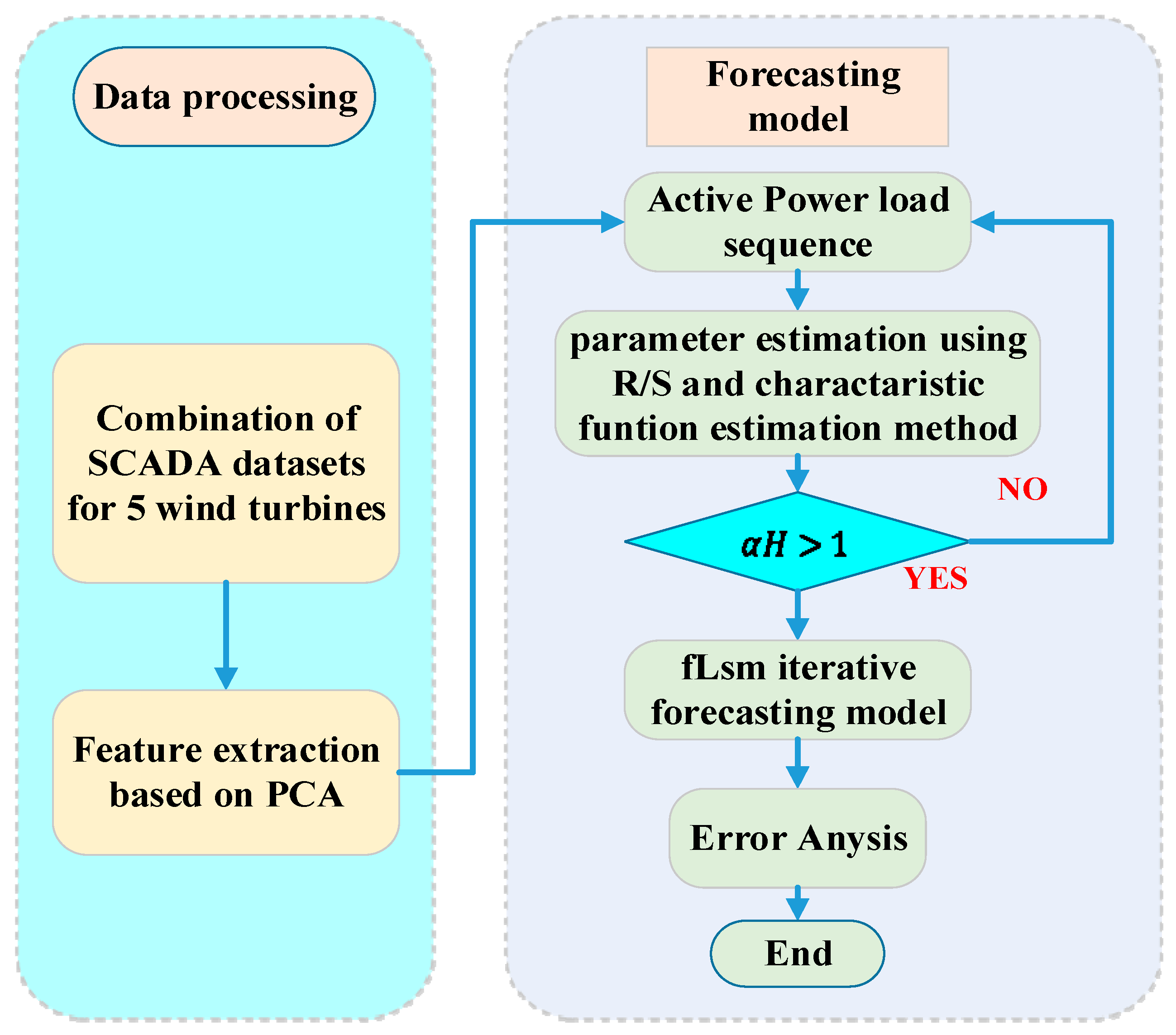
When wind turbine blades are encased in ice, it results in a reduction in power output. For the experiment, two specific time periods were selected as historical feature data: 26 December 2018 from 7:00 to 19:00 and 28 December 2018 from 7:00 to 19:00. The objective was to forecast the optimal wind energy generation and determine the icing trend. The overall experimental process is illustrated in Figure 4.
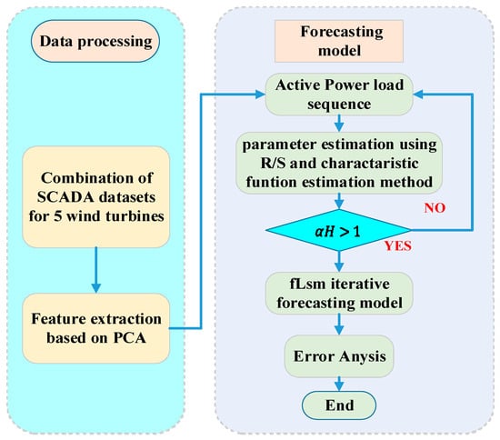
Figure 4.
Workflow for wind turbine blade icing prediction.
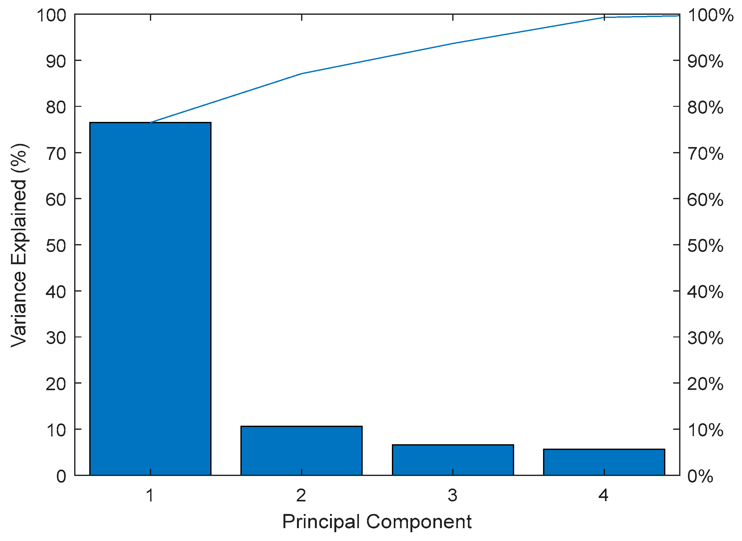
Firstly, there is a coupling relationship among the features in the original dataset. Therefore, before performing feature extraction and reconstruction, we used the PCA method to process the wind speed, the active power of the grid-side, the wind direction, and the temperature of the components of the turbine as input sequences. This resulted in a set of feature sequences with a better ice trend performance, with a cumulative contribution rate reaching 99.3132%, as shown in Figure 5. Secondly, we employed R/S and an improved maximum likelihood estimation method to estimate the model parameters for predicting 60 steps ahead for turbine A1. The specific parameter estimation results are shown in Table 3. It is worth noting that the value of parameter H is 0.8403 > 0.5, satisfying the condition for long-range dependence (LRD), thereby demonstrating the rationality of using the fLsm prediction model for modeling.
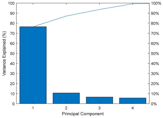
Figure 5.
Principal component analysis (PCA).
Table 3.
Parameter estimation results for a 60-step forecast model of wind turbine A1.
Therefore, the Lyapunov exponent estimated based on the small data method was 0.0111, and the maximum prediction range for icing trend was obtained as 90. This result provides crucial parameter support for the icing trend prediction model.
5.3. Prediction Results
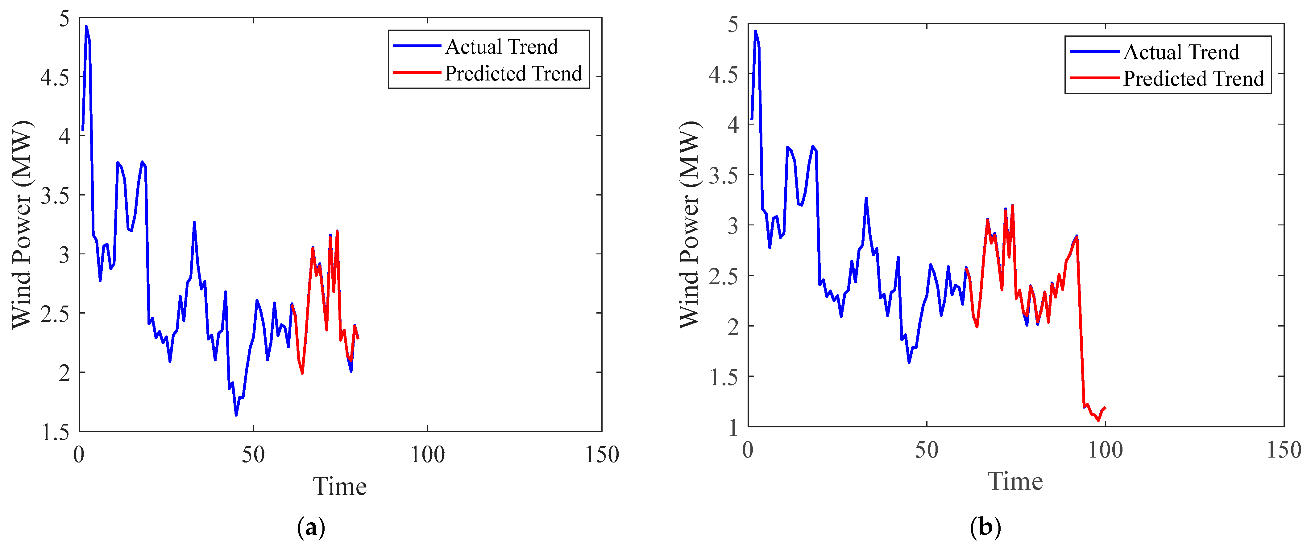
In this experiment, an iterative difference prediction model based on fLsm was employed to predict the power near icing conditions for the A1 wind turbine. Specifically, predictions were made for the A1 wind turbine for the next 20, 40, 60, and 80 steps, starting from the 60th step, regarding the trend of power changes. The predicted results are shown in Figure 6.
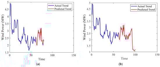
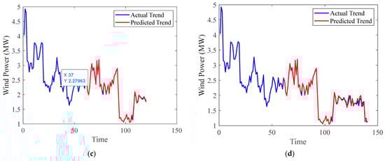
Figure 6.
A1 wind turbine icing trend power prediction results; (a) predicting 20 steps; (b) predicting 40 steps; (c) predicting 60 steps; (d) predicting 80 steps.
From the graph, it can be clearly observed that the fLsm iterative difference prediction model accurately predicts the icing trend of the A1 wind turbine at different prediction time steps. Comparing the model’s predicted results with actual data reveals a higher level of prediction accuracy, offering a viable approach for the timely forecasting of icing events. Additionally, it is noticeable that the prediction accuracy of the icing trend for the same set of sample sequences decreases as the prediction length increases. To analyze this trend in more detail, the model parameters for samples of different lengths are provided in Table 4.
Table 4.
Model parameters for samples of different prediction lengths.
5.4. Model Performance Analysis
In order to comprehensively evaluate the performance of the fLsm-based iterative difference prediction model, five evaluation metrics including maximum value, mean, standard deviation, SOA (accuracy score), and HD (Healthiness Index) were employed for performance analysis. The specific numerical results are presented in Table 5.
Table 5.
Performance analysis of the prediction model.
Through the error analysis presented in Table 5, the following conclusions can be drawn:
- (1)
- Maximum Value and Mean: The maximum value and mean, respectively, gauge the peak and overall level of prediction errors. From the data in the table, it can be observed that with an increase in prediction length, the maximum value gradually increases, while the mean remains relatively small. This indicates that, in certain scenarios, prediction errors may exhibit significant fluctuations, but the overall level remains at a relatively low magnitude.
- (2)
- Standard Deviation: The standard deviation reflects the dispersion of prediction errors. As the prediction length increases, the standard deviation gradually expands, indicating a broader range of prediction errors.
- (3)
- SOA (Accuracy Score) and HD (Healthiness Index): SOA and HD are metrics evaluating the overall performance of the model, considering both the accuracy and stability of predictions. With an increase in prediction length, both SOA and HD gradually decrease, indicating a decline in the overall performance of the model with the extension of the prediction length.
Overall, the fLsm-based iterative difference model demonstrates a certain effectiveness in predicting icing trends. In practical applications, flexibility in selecting prediction length is essential to strike a balance according to specific requirements, achieving a well-rounded performance. This is crucial for the timely and accurate prediction of icing events.
5.5. Model Comparison
5.5.1. Comparative Analysis of Model Prediction Result
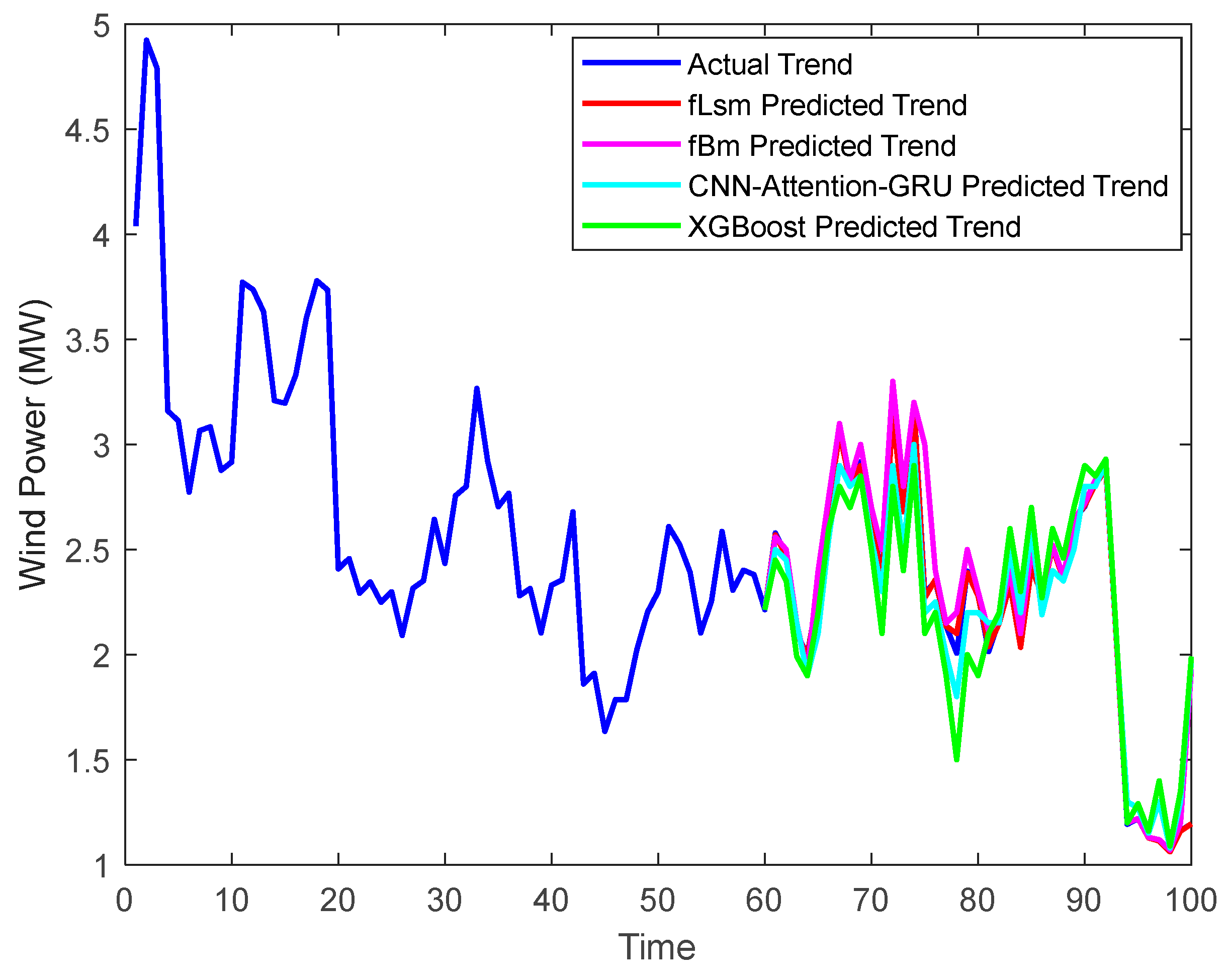
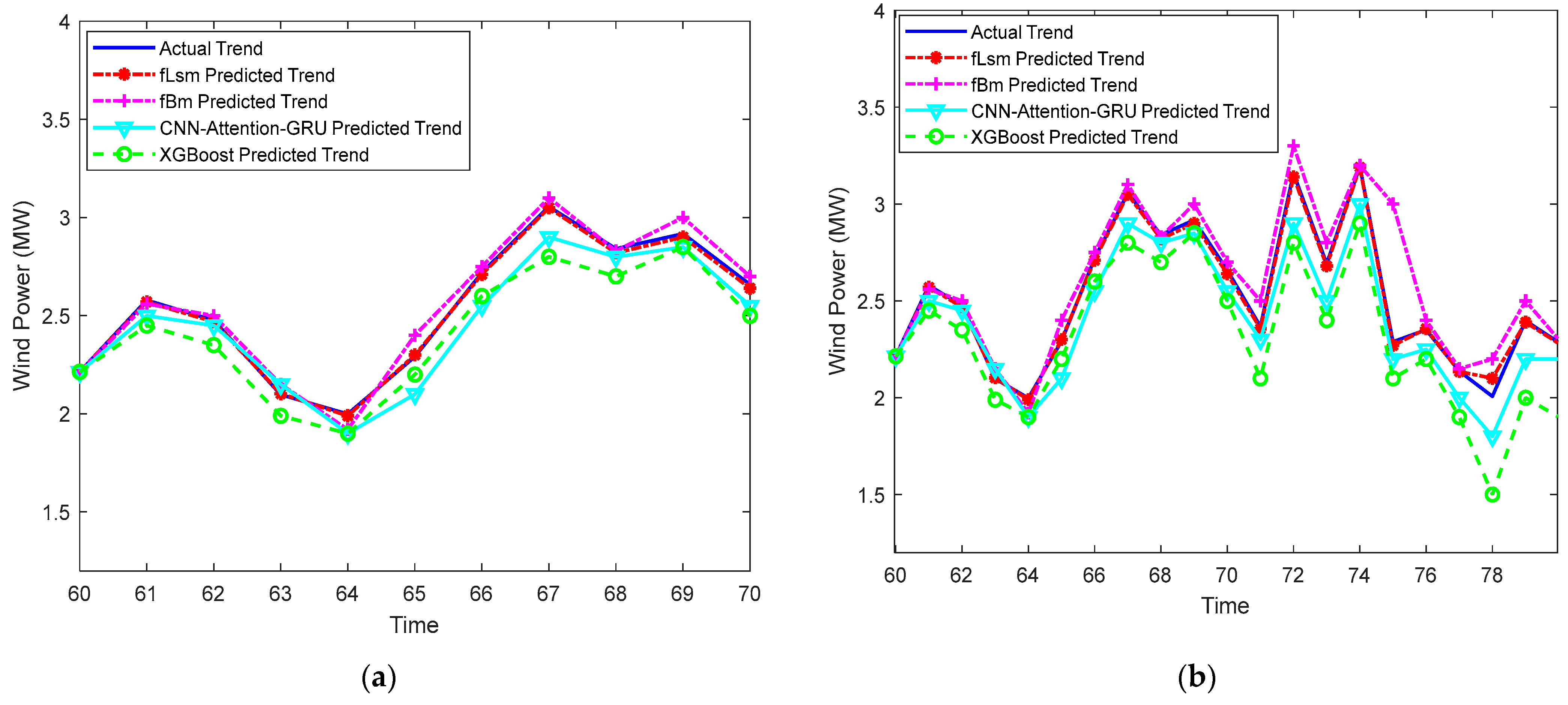
For the historical data encompassing the icing characteristics from 7:00 to 19:00 on 28 December 2018, various predictive models, including FBm, CNN-Attention-GRU, and XGBoost, were introduced for the prediction of 40 steps of feature power values. The results are depicted in Figure 7, where Figure 8a,b specifically illustrate the outcomes for 10 steps and 20 steps of prediction, respectively.
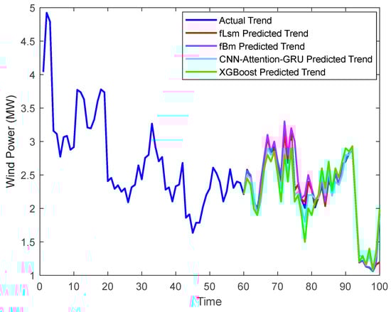
Figure 7.
Predicted trends by different models.

Figure 8.
Model comparison between [60, 70] and [60, 80] steps: (a) 10 steps; (b) 20 steps.
5.5.2. Performance Comparison of Different Models
The fLsm iterative difference prediction model was employed to forecast the power and icing state from 20:00 to 21:00 on 29 December 2018, utilizing the icing characteristics of five wind turbines during the period from 7:00 to 19:00 on the same day as historical data. The performance was compared with other models, such as FBm, CNN-Attention-GRU, and XGBoost. The results are presented in Table 6, with bold font highlighting the highest prediction accuracy achieved by each model in the respective dataset.
Table 6.
Icing prediction results for the four models.
Based on the analysis of experimental results, Table 6 demonstrates that the fLsm iterative difference prediction model exhibits higher accuracy in both power and icing state predictions compared to other models. Considering a comprehensive evaluation that combines accuracy and F1 score assessment, the fLsm model consistently demonstrates outstanding performance in power and icing state predictions across different wind turbine units. The F1 score represents the comprehensive performance of icing prediction results, being the harmonic mean of precision and recall. Precision measures the proportion of actual icing among the data predicted as icing by the model, while recall measures the proportion of actual icing data correctly predicted as icing by the model. A higher F1 score indicates better icing prediction capability of the model.
6. Conclusions
This study proposes a finite iterative wind turbine blade icing prediction method based on PCA-fLsm, demonstrating high accuracy and performance in experiments and holding significant potential for practical applications. The key conclusions of this research are as follows:
Criticality of Data Processing: Due to the multitude of operational signal features in wind turbines and the dynamic nature and data imbalance characteristics of blade icing faults, the application of principal component analysis (PCA) for high-dimensional data reduction and feature selection resolves data imbalance issues, enhancing model robustness.
LRD Characteristics of Icing Feature Sequences: The relationship between the Hurst parameter and feature index reveals the long-range dependence (LRD) characteristics of icing feature sequences, laying the foundation for modeling and aiding in promoting a better understanding of icing behavior.
Parameter Estimation Using New Feature Function Method: Successful utilization of the new feature function method estimates parameters of the fLsm model, including the stability index, skewness index, drift coefficient, and diffusion parameter, laying a foundation for establishing a reliable predictive model.
Superiority of fLsm Iterative Difference Prediction Model: The fLsm-based iterative difference prediction model demonstrates outstanding performance in handling wind turbine icing events, particularly under optimized conditions for sample length and the prediction step, improving accuracy in predicting power icing trends.
Introduction of Lyapunov Coefficient: The introduction of the Lyapunov coefficient effectively addresses accuracy issues in predictive models caused by nonlinearity and random factors, determining the maximum range for power predictions.
Comparison with Other Models: Through comparisons with FBm, CNN-Attention-GRU, and XGBoost models, the PCA-fLsm model proves superior and versatile in describing wind turbine icing SCADA data, achieving higher levels of accuracy.
In summary, this research provides a viable method for accurate prediction of wind turbine blade icing, ensuring both the effectiveness and precision of predictive data, thereby ensuring the safe, efficient, and stable operation of wind farms.
Author Contributions
F.C.: conceptualization, methodology, software, writing—original draft. Y.J.: writing—review and editing, methodology. T.Z.: formal analysis, data curation. W.S.: Project administration, Resources, Supervision. K.-H.L.: Funding acquisition, Supervision, Software. All authors have read and agreed to the published version of the manuscript.
Funding
This research was funded by the Science and Technology Project of Fujian Province (Grant No. 2023H6026, JAT220420) and the key science and technology project and science and technology innovation team of Minnan Institute of Technology, Joint Open-ended Foundation of State Key Laboratory of Integrated Automation in Process Industry of Northeastern University (grant number 22KJX007, 23XTD112, 2022-KF-21-02).
Data Availability Statement
Wind farms have confidentiality requirements regarding their data, and we cannot publish the data we have used.
Acknowledgments
The authors would like to thank the anonymous reviewers who gave valuable suggestions that have helped to improve the quality of the manuscript.
Conflicts of Interest
The authors declare no conflicts of interest.
References
- Awada, A.; Younes, R.; Ilinca, A. Review of Vibration Control Methods for Wind Turbines. Energies 2021, 14, 3058. [Google Scholar] [CrossRef]
- Li, Y.; Sun, C.; Jiang, Y.; Feng, F. Scaling Method of the Rotating Blade of a Wind Turbine for a Rime Ice Wind Tunnel Test. Energies 2019, 12, 627. [Google Scholar] [CrossRef]
- Thango, B.A.; Bokoro, P.N. Prediction of the Degree of Polymerization in Transformer Cellulose Insulation Using the Feedforward Backpropagation Artificial Neural Network. Energies 2022, 15, 4209. [Google Scholar] [CrossRef]
- Wei, K.; Yang, Y.; Zuo, H.; Zhong, D. A Review on Ice Detection Technology and Ice Elimination Technology for Wind Turbine. Wind Energy 2020, 23, 433–457. [Google Scholar] [CrossRef]
- Homola, M.C.; Virk, M.S.; Nicklasson, P.J.; Sundsbø, P.A. Performance losses due to ice accretion for a 5 MW wind turbine. Wind Energy 2012, 15, 379–389. [Google Scholar] [CrossRef]
- Xiao, J.; Li, C.; Liu, B.; Huang, J.; Xie, L. Prediction of Wind Turbine Blade Icing Fault Based on Selective Deep Ensemble Model. Knowl.-Based Syst. 2022, 242, 108290. [Google Scholar] [CrossRef]
- Li, N.; Yan, T.; Li, N.; Kong, D.; Liu, Q.; Lei, Y. Ice Detection Method by Using SCADA Data on Wind Turbine Blades. Power Gener. Technol. 2018, 39, 58–62. [Google Scholar]
- Jiang, G.; Yue, R.; He, Q.; Xie, P.; Li, X. Imbalanced Learning for Wind Turbine Blade Icing Detection via Spatio-Temporal Attention Model with a Self-Adaptive Weight Loss Function. Expert Syst. Appl. 2023, 229, 120428. [Google Scholar] [CrossRef]
- Li, F.; Cui, H.; Su, H.; Ma, Z.; Zhu, Y.; Zhang, Y. Icing Condition Prediction of Wind Turbine Blade by Using Artificial Neural Network Based on Modal Frequency. Cold Reg. Sci. Technol. 2022, 194, 103467. [Google Scholar] [CrossRef]
- Geng, Y.; Wang, Z.; Jia, L.; Qin, Y.; Chen, X. Bogie Fault Diagnosis under Variable Operating Conditions Based on Fast Kurtogram and Deep Residual Learning towards Imbalanced Data. Measurement 2020, 166, 108191. [Google Scholar] [CrossRef]
- Wright, L.G.; Onodera, T.; Stein, M.M.; Wang, T.; Schachter, D.T.; Hu, Z.; McMahon, P.L. Deep physical neural networks trained with backpropagation. Nature 2022, 601, 549–555. [Google Scholar] [CrossRef]
- Chen, Q.; Folly, K.A. Wind power forecasting. IFAC-PapersOnLine 2018, 51, 414–419. [Google Scholar] [CrossRef]
- Tao, T.; Liu, Y.; Qiao, Y.; Gao, L.; Lu, J.; Zhang, C.; Wang, Y. Wind Turbine Blade Icing Diagnosis Using Hybrid Features and Stacked-XGBoost Algorithm. Renew. Energy 2021, 180, 1004–1013. [Google Scholar] [CrossRef]
- Zhang, D. Research on the Prediction of Wind Turbine Blade Icing Based on a Hybrid model of LightGBM, XGBoost, and ERT. Ph.D. Dissertation, Shanghai Normal University, Shanghai, China, 2018. [Google Scholar]
- Chen, J.; Hu, W.; Cao, D.; Zhang, B.; Huang, Q.; Chen, Z.; Blaabjerg, F. An Imbalance Fault Detection Algorithm for Variable-speed Wind Turbines: A Deep Learning Approach. Energies 2019, 12, 2764. [Google Scholar] [CrossRef]
- Tao, C.; Tao, T.; Bai, X.; Liu, Y. Wind Turbine Blade Icing Prediction Using Focal Loss Function and CNN-Attention-GRU Algorithm. Energies 2023, 16, 5621. [Google Scholar] [CrossRef]
- Wang, C.; Li, H.; Zhang, K.; Hu, S.; Sun, B. Intelligent Fault Diagnosis of Planetary Gearbox Based on Adaptive Normalized CNN under Complex Variable Working Conditions and Data Imbalance. Measurement 2021, 180, 109565. [Google Scholar] [CrossRef]
- Kreutz, M.; Alla, A.A.; Lütjen, M.; Ohlendorf, J.-H.; Freitag, M.; Thoben, K.-D.; Zimnol, F.; Greulich, A. Ice prediction for wind turbine rotor blades with time series data and a deep learning approach. Cold Reg. Sci. Technol. 2023, 206, 103741. [Google Scholar] [CrossRef]
- Xu, X.; Feng, T.; Cai, Z.; Tang, J.; Dai, W.; Wang, L.; Li, L.; Xu, M.; Cao, W. Analysis of a Wind Farm Icing Event Based on the In-situ Observation and Numerical Model Prediction. In Proceedings of the 2023 6th International Conference on Energy, Electrical and Power Engineering (CEEPE), Guangzhou, China, 12–14 May 2023; p. 10166967. [Google Scholar]
- Bai, X.; Tao, T.; Gao, L.; Tao, C.; Liu, Y. Wind Turbine Blade Icing Diagnosis Using RFECV-TSVM Pseudo-Sample Processing. Renew. Energy 2023, 211, 412–419. [Google Scholar] [CrossRef]
- Liu, B.; Feng, L. Improving the Accuracy of Lane Detection by Enhancing the Long-Range Dependence. Electronics 2023, 12, 2518. [Google Scholar] [CrossRef]
- Laskin, N.; Lambadaris, I.; Harmantzis, F.C.; Devetsikiotis, M. Fractional Levy motion and its application to network traffic modeling. Comput. Netw. 2002, 40, 363–375. [Google Scholar] [CrossRef]
- Wang, Q.; Yi, X.; Liu, Y.; Ren, J.; Li, W.; Wang, Q.; Lai, Q. Simulation and analysis of wind turbine ice accretion under yaw condition via an Improved Multi-Shot Icing Computational Model. Renew. Energy 2020, 162, 1854–1873. [Google Scholar] [CrossRef]
- Cheng, P.; Jing, H.; Hao, C.; Xinpan, Y.; Xiaojun, D. Icing Prediction of Fan Blade Based on a Hybrid Model. Int. J. Perform. Eng. 2019, 15, 2882. [Google Scholar] [CrossRef]
- Hu, Q.; Xu, X.; Leng, D.; Shu, L.; Jiang, X.; Virk, M.; Yin, P. A Method for Measuring Ice Thickness of Wind Turbine Blades Based on Edge Detection. Cold Reg. Sci. Technol. 2021, 192, 103398. [Google Scholar] [CrossRef]
- Abdoos, A.A. A new intelligent method based on combination of VMD and ELM for short term wind power forecasting. Neurocomputing 2016, 203, 111–120. [Google Scholar] [CrossRef]
- Putz, D.; Gumhalter, M.; Auer, H. A novel approach to multi-horizon wind power forecasting based on deep neural architecture. Renew. Energy 2021, 178, 494–505. [Google Scholar] [CrossRef]
- Zhang, D.; Tian, W.; Cheng, X.; Shi, F.; Qiu, H.; Liu, X.; Chen, S. FedBIP: A Federated Learning-Based Model for Wind Turbine Blade Icing Prediction. IEEE Trans. Instrum. Meas. 2023, 72, 3516011. [Google Scholar] [CrossRef]
- Samorodnitsky, G.; Taqqu, M. Stable non-Gaussian random processes: Stochastic models with infinite variance. J. Am. Stat. Assoc. 1995, 90, 805. [Google Scholar]
- Kogon, S.M.; Manolakis, D.G. Signal modeling with self-similar α-stable processes: The fractional levy stable motion model. IEEE Trans. Signal Process. 1996, 44, 1006–1010. [Google Scholar] [CrossRef]
- Rahimi, E.; Rabiee, A.; Aghaei, J.; Muttaqi, K.M.; Nezhad, A.E. On the management of wind power intermittency. Renew. Sustain. Energy Rev. 2013, 28, 643–653. [Google Scholar] [CrossRef]
- Zou, H.-L.; Yu, Z.; Anh, V.; Ma, Y.-L. From standard alpha-stable Levy motions to horizontal visibility networks: Dependence of multifractal and Laplacian spectrum. J. Stat. Mech. Theory Exp. 2018, 2018, 053403. [Google Scholar] [CrossRef]
- Liu, H.; Song, W.; Zio, E. Generalized Cauchy difference iterative forecasting model for wind speed based on fractal time series. Nonlinear Dyn. 2021, 103, 759–773. [Google Scholar] [CrossRef]
- Liu, H.; Song, W.Q.; Zio, E. Fractional Lévy stable motion with LRD for RUL and reliability analysis of li-ion battery. ISA Trans. 2022, 125, 360–370. [Google Scholar] [CrossRef] [PubMed]
- Marquardt, T. Fractional Lévy processes with an application to long memory moving average processes. Bernoulli 2006, 12, 1099–1126. [Google Scholar] [CrossRef]
- Duan, S.; Song, W.; Zio, E.; Cattani, C.; Li, M. Product technical life prediction based on multi-modes and fractional Lévy stable motion. Mech. Syst. Signal Process. 2021, 161, 107974. [Google Scholar] [CrossRef]
- Wang, X.; Li, K.; Gao, P.; Meng, S. Research on parameter estimation methods for alpha-stable noise in a laser gyroscope’s random error. Sensors 2015, 15, 18550–18564. [Google Scholar] [CrossRef]
- Song, W.; Liu, H.; Zio, E. Long-range dependence and heavy tail characteristics for remaining useful life prediction in rolling bearing degradation. Appl. Math. Model. 2022, 102, 268–284. [Google Scholar] [CrossRef]


Disclaimer/Publisher’s Note: The statements, opinions and data contained in all publications are solely those of the individual author(s) and contributor(s) and not of MDPI and/or the editor(s). MDPI and/or the editor(s) disclaim responsibility for any injury to people or property resulting from any ideas, methods, instructions or products referred to in the content. |
© 2024 by the authors. Licensee MDPI, Basel, Switzerland. This article is an open access article distributed under the terms and conditions of the Creative Commons Attribution (CC BY) license (https://creativecommons.org/licenses/by/4.0/).