Multi-Step Approach for Fast Calculation of Magnetic Field in Transformer Tank Shields

Abstract

A multi-step approach for the fast calculation of the magnetic field inside transformer tank shields, based on the 2D FEM, is presented in the paper. Due to the limitations of the 2D FEM, the proposed approach utilizes several 2D FEM models and calculates the magnetic field in multiple steps to account for the 3D geometry of the problem. In the first step, a distribution of the magnetic flux density that enters the tank shields is calculated using the quasi-3D model of the transformer. This quasi-3D model is obtained by superimposing the solution of multiple axisymmetric 2D FEM models, and assumes a considerably simplified transformer geometry. To account for the tank shield geometry that is neglected in the quasi-3D FEM model, an additional 2D FEM model with tank shields is introduced. After the distribution of the magnetic flux density that enters the tank shields is calculated, it is imposed in the final 2D FEM model with a non-linear tank shield which is used to calculate the magnetic flux density distribution inside the tank shields. The proposed approach enables a fast calculation of magnetic field distributions, both in the vertical and horizontal directions. The results of the proposed approach are compared against the 3D FEM. The relative error of the maximum magnetic flux density is under 2%, while the NRMSE of the magnetic flux density distribution within the tank shields is under 10%. The key contribution of the proposed approach is a low computation time. In the presented case study, the total computation time of the proposed approach is ~30 s, while the computation time of the 3D FEM is ~1 h. As the computation time is significantly reduced, while the accuracy is acceptable, the proposed approach can be a good alternative to the 3D FEM for design purposes. Therefore, it has industrial value.

1. Introduction

In power transformers, the leakage magnetic field causes stray losses in the structural parts, such as the tank or the clamping system. The issue of stray losses is addressed in a review article [1] that states that stray losses remain an active research area both in universities and in industry. It emphasizes the importance of reducing stray losses in power transformers. Another important issue related to stray losses is overheating. A paper [2] investigates the impact of overheating on insulation, which is crucial for the normal operation of a transformer. A well-established method for reducing stray losses and overheating is the use of magnetic shielding, achieved through the deployment of flux collectors.

References are provided below that address the usage and efficiency of flux collectors in power transformers. Reference [3] analyzes the impact of tank shields on stray losses in a tank using the 3D finite element method (FEM) and its measurements. The results have shown a reduction in tank losses by 12%. Reference [4] investigates the effect of lobe-type magnetic shielding, using a 334 MVA single-phase auto-transformer as an example. The 3D FEM results, validated by experimental data, demonstrate a loss reduction in the main structural parts by 30%. A loss reduction of 63.6% is reported in Reference [5]. In Reference [6], a comparison between the horizontal and vertical tank shields is presented, based on a 200 MVA transformer and utilizing the 3D FEM. The study reveals that both types of shields are equally effective, reducing losses by approximately 80%. However, horizontal shields weigh 25% less than vertical shields. This reference also explores the optimization of the shield placement on the tank walls. In Reference [7], a case study is conducted on a 315 MVA single-phase generator transformer, employing a coupled electromagnetic–thermal 3D FEM. The use of vertical shields, yoke shunts, and limb shunts resulted in a 64% reduction in stray losses and a 15 °C decrease in temperature hotspots. Additionally, the analysis indicates that magnetic shielding is significantly more effective compared to electromagnetic shielding. The cited references support the effectiveness of magnetic shielding methods, which are well-established and widely used in power transformers.

The geometry of magnetic flux collectors is optimized during the transformer design phase. Geometry optimization is based on the magnetic flux density within the flux collector, and several approaches are used in practice. The magnetic field in flux collectors can be calculated using the 2D or 3D FEM. Apart from optimization based on the calculated field values, in some cases, the collector geometry parameters are chosen following specific guidelines. Reference [8] suggests that using empirical equations during the design phase is preferable due to the low computation time required. It also proposes design rules for tank shields and yoke shunts. Reference [9] introduces the application of a 3D mixed FEM–BEM method to optimize the geometry of magnetic shields. Reference [10] utilizes 2D and 3D FEM models to optimize the placement and geometry of the tank shield. In all cited references, analyses were conducted using the 3D FEM due to the three-dimensional geometry of the problem. However, the high computational resources and computation time required by the 3D FEM render it unfavorable for the transformer design phase.

The authors proposed a multi-step approach for the fast calculation of the magnetic field in the power transformer yoke shunt in Reference [11]. The approach uses multiple 2D FEM models with different cross-sections to account for the three-dimensional geometry of the problem. Importantly, these models require low computational resources and computation time, making them suitable for the design phase. In this paper, a multi-step approach is applied to the calculation of the magnetic field in vertical tank shields. Due to the significant difference in the yoke shunt’s and the vertical tank shields’ geometries, the multi-step approach from [11] cannot be directly applied and requires modifications.

The authors did not find any similar research in the previous literature that addresses the calculation of the 3D magnetic field in flux collectors using 2D FEM models. However, there are several references where 3D problems are solved using 2D models with an application to other problems in transformers. An often-used term for such modeling techniques is quasi-3D modeling. Examples of quasi-3D modeling are given in the references below. The authors proposed a quasi-3D modeling technique for the calculation of stray losses in the outer lamination stacks of the transformer core in Reference [12]. Reference [13] proposes a quasi-3D coupled electromagnetic–thermal calculation of the temperature rise in a dry-type transformer. Reference [14] proposes an analytical hybrid quasi-3D model for the calculation of the leakage inductance of core-type transformers. In References [15,16], quasi-3D models for the calculation of the leakage inductance and the current distribution in parallel-connected windings, respectively, are proposed. These models are based on conformal mapping and allow a non-symmetric geometry with windings on different core legs, which is a case in some special transformers. What is common to the proposed approach and the methods from the cited References [12,13,14,15,16] is that they calculate 3D problems using multiple 2D models with different cross-sections. In addition to the mentioned examples of the quasi-3D modeling of transformers, several examples of the quasi-3D modeling of electrical motors and generators are provided in References [17,18,19,20,21].

The function of tank shields in power transformers is explained in Section 2. Section 3 presents the magnetic field calculation within these shields, employing both well-established 2D FEM and 3D FEM models, as well as the multi-step approach. Section 4 compares the proposed approach to the 3D FEM using a real power transformer geometry. Finally, Section 5 and Section 6 provide the discussion and conclusion.

2. Vertical Tank Shields

Vertical tank shields are a type of magnetic flux collector positioned on the tank walls of a power transformer. Their purpose is to redirect stray flux away from the tank walls, thereby reducing losses and heating. These tank shields are constructed from highly permeable steel lamination stacks. Figure 1 illustrates the geometry of the vertical tank shields within the power transformer.

The magnetic flux density within a well-designed tank shield should not exceed the saturation point of the shield material. Additionally, the magnetic flux density distribution within the shield should be as uniform as possible to optimize the use of the steel material efficiently. In most cases, the design of the tank shields considers the vertical non-uniformity of the magnetic flux while ignoring the horizontal non-uniformity [22] (Chapter 5.9.1). Calculating the magnetic flux distribution density within the tank shield is necessary in order to optimize the tank shield’s geometry.

3. Calculation of Magnetic Field in Tank Shields

This section presents a calculation of the magnetic field within the tank shields. First, the field calculation using the standard FEM models is explained. Then, a field calculation using the multi-step approach is proposed.

3.1. Standard FEM Models

The magnetic field within the vertical tank shields can be calculated using three types of FEM models. The most accurate among these models is the 3D FEM model. In this case, the transformer’s geometry can be modeled in detail, as illustrated in Figure 1. However, the drawbacks of the 3D FEM are the long computation time, the high computational resource requirements, and the implementation complexity.

The other two types of FEM models are planar and axisymmetric 2D FEM models, which require significantly less computation time and fewer computational resources, and are easier to implement compared to the 3D FEM model. However, these models assume a simplified geometry, which reduces their accuracy. The planar 2D FEM model assumes an infinitely long geometry, resulting in higher magnetic field values within the tank shields compared to the 3D FEM model, whereas the assumption of an axisymmetric geometry leads to lower field values.

Therefore, this paper aims to develop a procedure for calculating the magnetic field within tank shields using 2D FEM models to ensure a low computation time. The procedure requires multiple 2D FEM models with various cross-sections to account for the 3D geometry of the problem.

All FEM models used in this paper are magnetostatic, as there is no need to calculate the eddy currents. The following FEM software is used:

• Simcenter MAGNET 2020.1 is used for all 3D FEM calculations.

  ◦

  Magnetostatic problems are formulated using the scalar magnetic potential.

  ◦

  Second-order tetrahedral elements are used.

  ◦

  In this paper, the windings in the 3D model are current-driven.

• FEMM 4.2 [23] is used for all 2D FEM calculations.

  ◦

  Magnetostatic and quasi-magnetostatic problems in this software are formulated using the vector magnetic potential. In the case of 2D models, the vector magnetic potential has only one vector component, which is perpendicular to the 2D plane. Therefore, it is denoted by the letter A as a scalar throughout the paper.

  ◦

  First-order triangular elements are used.

  ◦

  In this paper, two types of sources are used in 2D FEM models:

  ▪

  In models that include windings, the currents are defined in these windings.

  ▪

  In other models that do not include windings, the magnetic field is imposed by defining a vector magnetic potential, as explained later in the paper (Section 3.4).

  ◦

  In this paper, the pre-processing and post-processing are scripted using MATLAB R2020b.

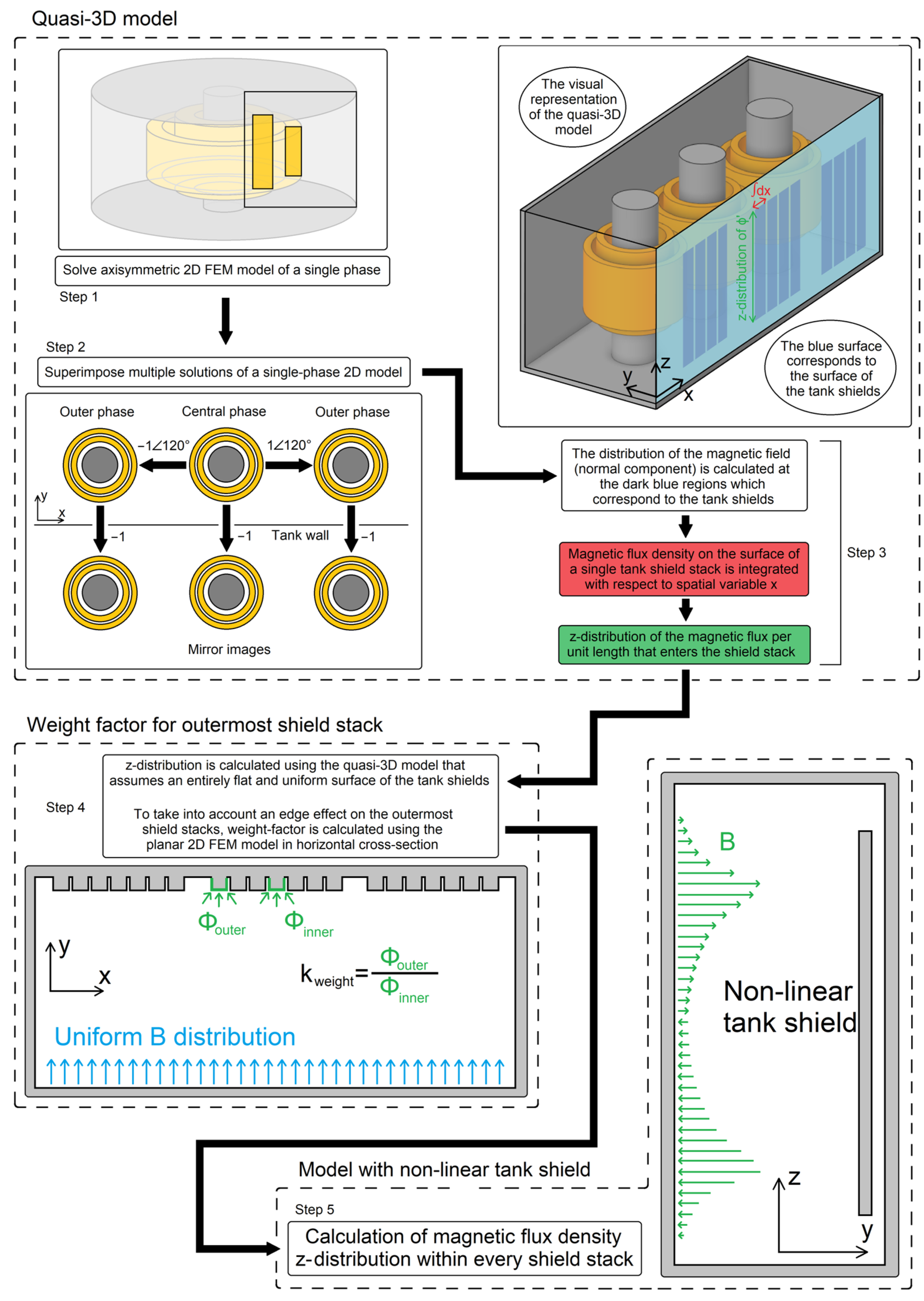
3.2. Multi-Step Calculation

A brief overview of the proposed procedure’s calculation steps is provided in this subsection. For clarity, the calculation steps are explained through the flow diagram shown in Figure 2. The 2D FEM models used in the calculation steps are as follows:

• A single-phase axisymmetric 2D FEM model that includes the windings and core is used (Step 1 in Figure 2 and more detailed explanation in Figure 3a).

  ◦

  The solution is superimposed multiple times to obtain a quasi-3D model (Step 2 in Figure 2 and more detailed explanation in Figure 3b).

  ◦

  The method of mirror images is used to simulate permeable tank shields.

  ◦

  This model is used to calculate the magnetic field on the surface of the tank shields (Step 3 in Figure 2), which is explained in detail in Section 3.3.

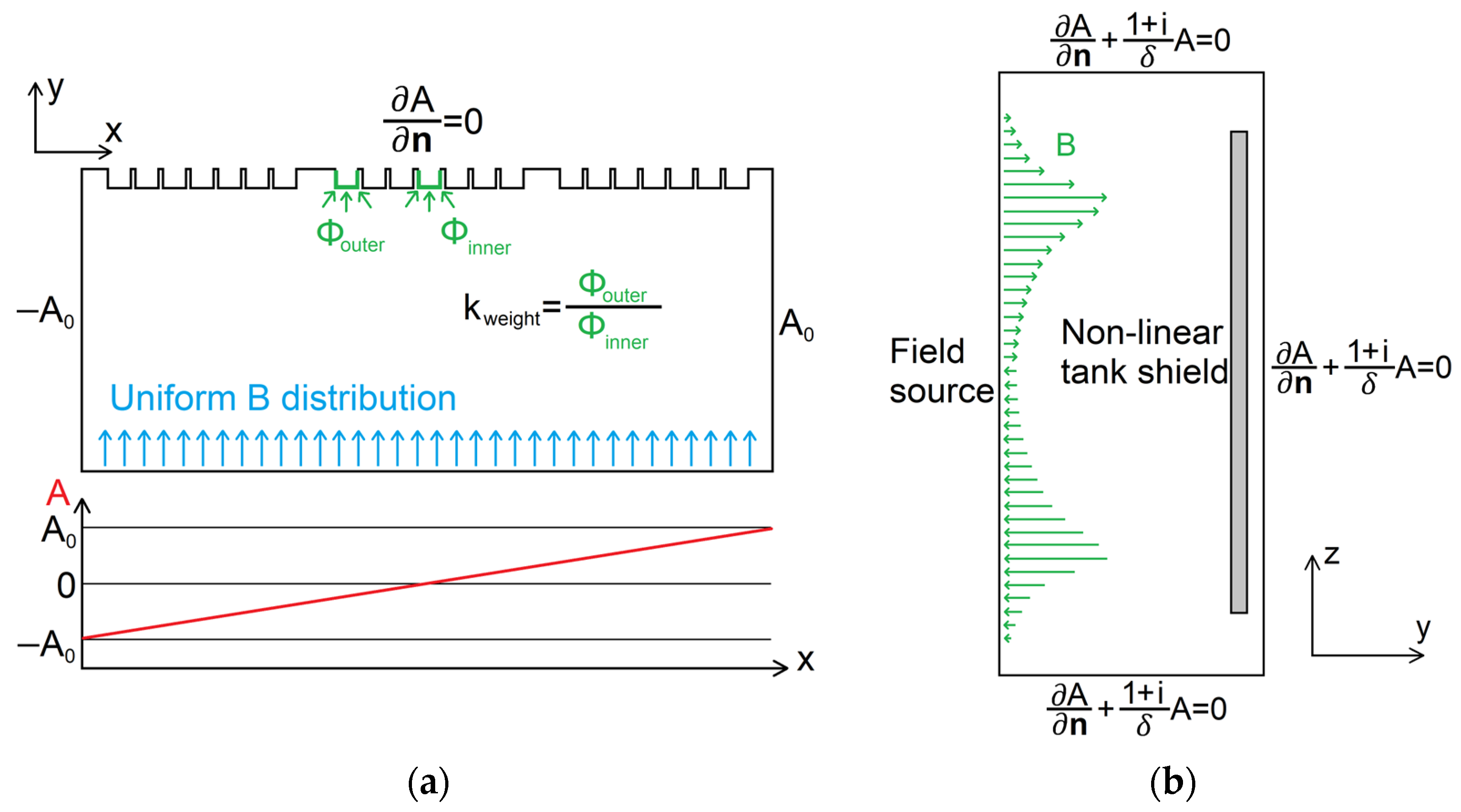
• A 2D FEM model in the horizontal cross-section, with a detailed geometry of tank shields, is used to calculate the weight factors (Step 4 in Figure 2). These factors determine how much of the magnetic flux, calculated with a quasi-3D model, enters the particular tank shield stack. This step is explained in detail in Section 3.5.
• A 2D FEM model in a vertical cross-section with a non-linear tank shield calculates the vertical distribution of the magnetic flux density within the tank shield stack (Step 5 in Figure 2). This step must be carried out for every single stack. It is explained in detail in Section 3.6.

The detailed explanations of all steps are given in the rest of the section.

Figure 2. Flow diagram of multi-step procedure.

Figure 2. Flow diagram of multi-step procedure.

Figure 3. Quasi-3D model: geometry of an axisymmetric 2D FEM model of a single phase (a); geometry of quasi-3D model (b); and procedure for superimposing original solutions (c).

Figure 3. Quasi-3D model: geometry of an axisymmetric 2D FEM model of a single phase (a); geometry of quasi-3D model (b); and procedure for superimposing original solutions (c).

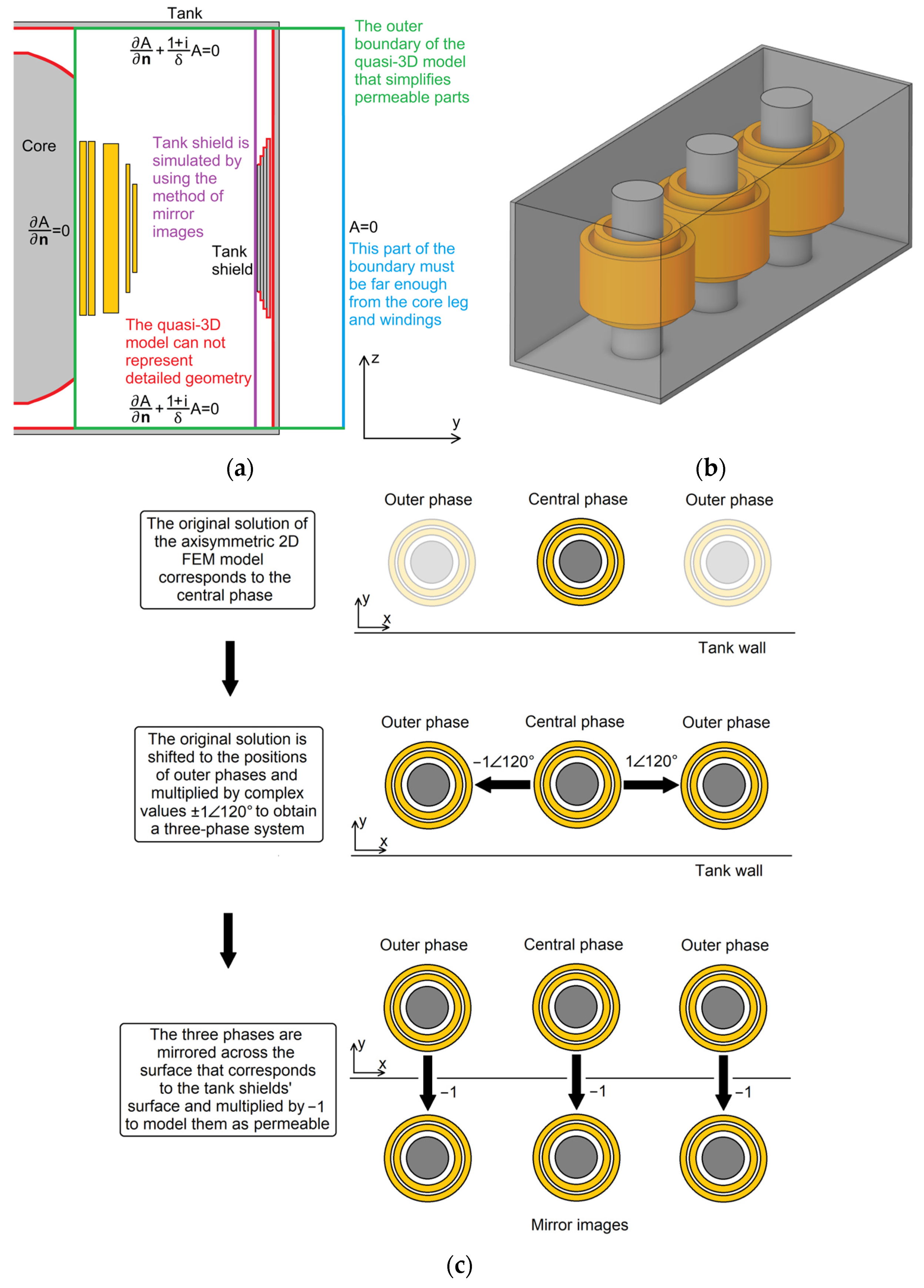
3.3. Quasi-3D Model

The first step of the multi-step approach involves calculating the magnetic field on the surface of tank shields. To account for the 3D geometry of the transformer, a quasi-3D model of the core, tank, and the three-phase system of windings is employed. This quasi-3D model is derived by superimposing multiple solutions of an axisymmetric 2D FEM model of a single phase (see Figure 3a), as explained in this subsection. The use of superposition is valid, as the magnetic field in the air (linear material) is calculated in this step.

In this step, the magnetic field on the surface of laminated, highly permeable tank shields is a value of interest. When the magnetic field outside the laminated magnetic material is a value of interest, that material can be modeled as infinitely permeable as explained in Reference [24]. In that case, there is no tangential component of the magnetic field on surface. In the quasi-3D model, the core leg and tank shields are laminated and assumed to be infinitely permeable. The core leg is modeled using an appropriate boundary condition, and the tank shields are modeled using the method of mirror images, which is explained below.

In magnetostatic problems formulated through the vector magnetic potential $A$, the cancellation of the tangential field component is obtained by applying the Neumann boundary condition $\frac{\partial A}{\partial \mathit{n}}=0$. The core leg is modeled using this boundary condition (inner boundary marked green in Figure 3a). As the tank is not laminated, its eddy currents can have some impact on the field distribution. Therefore, the surface impedance boundary condition $\frac{\partial A}{\partial \mathit{n}}+\frac{1+i}{\delta }A=0$ is used to model the bottom and the top of the tank (top and bottom boundaries marked green in Figure 3a). Reference [25] addresses the modeling of conductive materials using surface boundary conditions.

The quasi-3D model is based on the solution of an axisymmetric 2D FEM model of a single phase (see Figure 3a). This model includes windings, where the inner (left) boundary represents the core leg, and the top and bottom boundaries correspond to the top and bottom of the tank, respectively. The outer (right) boundary (outer boundary marked blue in Figure 3a) does not correspond to any part of the transformer and, ideally, should be infinitely far away from the core leg. The authors set the outer boundary at a distance of one tank length, which proved to be sufficient so that this boundary does not affect the field near the windings.

The quasi-3D model is obtained by superimposing multiple axisymmetric 2D FEM models (see Figure 3c) as follows:

The central axes of these three models correspond to the central axes of all three core legs, with the phase shifts of the complex-valued currents (phasors) in the windings being $-120°$, $0°$, and $120°$, respectively.

The method of mirror images is used to simulate planar, infinitely permeable tank shields. Consequently, the previously mentioned three models are mirrored across a plane corresponding to the surface of the tank shields (this surface is marked green in Figure 3a and blue in Step 3 in Figure 2), with currents in the original and mirrored models having opposite directions. Examples of employing the method of mirror images in magnetostatic problems are provided in References [26,27].

Since all these 2D FEM models share the same geometry, solving only one 2D FEM model is necessary, with the complete solution obtained in post-processing. The geometry of the quasi-3D model is shown in Figure 3b.

It is important to note that the proposed approach assumes short-circuit test conditions. Therefore, in this step, the sum of the ampere-turns in the windings must be equal to zero.

3.4. Imposing an Arbitrary Magnetic Flux Density Distribution in a 2D FEM Model

The two steps of the proposed procedure require imposing an arbitrary magnetic flux density distribution on the outer boundary of the 2D FEM model, which is explained in this subsection.

In general, a relation between the vector magnetic potential and the magnetic field is expressed as follows:

$$\mathit{B}=\nabla \times \mathit{A},$$

(1)

which is valid for the 3D geometry and field $\mathit{B}$ that has all spatial components. In this paper, a case of interest involves the magnetic flux density $B_n$ that is perpendicular to the 2D problem boundary. In that case, Expression (1) can be simplified to the following:

$$B_n\left(x_{tan}\right)=\frac{dA\left(x_{tan}\right)}{d{x}_{tan}},$$

(2)

where $x_{tan}$ is the spatial variable tangential to both the boundary and computation plane, and $A$ is the component of the vector magnetic potential, normal to the 2D FEM computation plane (there are no other spatial components of field $\mathit{A}$ in the 2D model). Both $B_n$ and $A$ are a function of the spatial variable $x_{tan}$. To impose an arbitrary distribution of the magnetic flux density $B_n\left(x_{tan}\right)$ on a specific boundary, we define the distribution of the vector magnetic potential $A\left(x_{tan}\right)$ that is obtained by integrating Expression (2):

$$A\left(x_{tan}\right)=\int B_n\left(x_{tan}\right)d{x}_{tan}.$$

(3)

3.5. Calculation of the Weight Factors Using the Horizontal 2D FEM Model

The magnetic flux density on the surface of the tank shields is calculated using the quasi-3D model that neglects the detailed geometry of the tank shields. The weight factors are introduced in order to consider the geometry of the tank shield stacks in the horizontal cross-section (x–y plane in Figure 1). These factors determine how much of the previously calculated magnetic flux enters the outermost stacks. Due to the discontinuity in the geometry at the shield’s edge, the flux values that enter the outermost stacks are increased compared to the inner stacks.

In the horizontal 2D FEM model (see Figure 4a), the y-co-ordinate of the bottom boundary is in the middle between the windings and tank shields. The uniform flux density distribution (marked by blue arrows in Figure 4a) of arbitrary magnitude is imposed on the bottom boundary using Expression (3), as explained in the previous subchapter. The boundary condition $\frac{\partial A}{\partial \mathit{n}}=0$ is applied to the upper boundary to model the permeable tank shields. The vector magnetic potential is constant on the left and right boundaries to achieve a parallel flux.

The weight factor is calculated for the outermost stacks, while it equals 1 for the inner stacks. For the outermost stacks, the weight factor is calculated as the ratio of the flux entering the outermost stack and the central stack.

3.6. Calculation of Magnetic Flux Density within the Tank Shield Using the Vertical 2D FEM Model

The final step is calculating the magnetic flux density within the tank shield stacks. First, the vertical distribution of the magnetic flux (per unit length) that enters the shield stacks is calculated using the following expression:

$${{\mathrm{ф}}^{\prime }}_{stack}\left(z\right)={\int }_{leftsideofstack}^{rightsideofstack}{B}_z\left(x,z\right)·k_{weight}dx.$$

(4)

The integration with respect to the x variable is illustrated in Step 3 in Figure 2. $B_z\left(x,z\right)$ is the magnetic flux density on the surface of the tank shields (marked blue in Step 3 in Figure 2) calculated using the quasi-3D model, whereas the $k_{weight}$ is the weight factor introduced in Section 3.5.

The flux density distribution,

$$B_{stack}\left(z\right)=\frac{1}{w_{stack}}{{\mathrm{ф}}^{\prime }}_{stack}\left(z\right),$$

(5)

is imposed in the vertical 2D FEM model with non-linear tank shields (see Figure 4b). The parameter $w_{stack}$ in Expression (5) is the width of the shield stack. In the vertical 2D FEM model (plane y–z in Figure 1), the tank is represented by the outer boundary where the surface impedance boundary condition is applied (top, bottom, and right boundary in Figure 4b). The flux density distribution $B_{stack}\left(z\right)$ is imposed on the left boundary (marked by green arrows in Figure 4b), as proposed in Section 3.4. The y-co-ordinate of the left boundary is the same as in the model for the weight factor calculation.

4. Case Study

The proposed approach is used to calculate the magnetic flux density in tank shields on the example of a real three-phase power transformer geometry. The flux density is calculated on both the low-voltage (LV) and high-voltage (HV) sides. For this particular transformer, eighteen 2D FEM models were used in the multi-step approach. These include a quasi-3D model, a model for the weight factor calculation, and sixteen non-linear models for each shield stack. The detailed geometry of the transformer is confidential data. Therefore, only some basic information about the transformer is given in

Table 1. Transformer data.

Parameter	Value
Rated power	300 MVA
Frequency	50 Hz
Voltage level	220/20 kV
Short-circuit impedance	14%
Core type	3–2

. The results of the proposed approach are compared against the results of the 3D FEM calculation.

The 2D distributions of the magnetic flux density at a distance of 100 mm from the blue plane (see Figure 2) and perpendicular to it are calculated using the quasi-3D model and 3D FEM, and are shown in Figure 5. The distributions of the magnetic flux density within the shield, calculated using the 3D FEM, the planar 2D FEM, the axisymmetric 2D FEM, and the proposed multi-step approach, are shown in Figure 6.

The maximum values of the flux density within the shields are compared using the relative error:

$$\epsilon =\frac{B_{2D}-B_{3D}}{B_{3D}},$$

(6)

and the 2D distributions of the flux density within the shields are compared using the normalized root–mean–square error (NRMSE):

$$NRMSE=\sqrt{\frac{{\int }_{x_1}^{x_2}{\int }_{z_1}^{z_2}{\left({|B}_{2D}\left(x,z\right)|-{|B}_{3D}\left(x,z\right)|\right)}^{2}dxdz}{{{|B}_{3D,max}|}^2·(x_2-x_1)·(z_2-z_1)}},$$

(7)

where $x_1$, $x_2$, $z_1$, and $z_2$ are the co-ordinates between which the distribution is considered and $B_{2D}$ and $B_{3D}$ are the values calculated using the 2D and 3D models, respectively. A comparison of the 2D FEM results to the 3D FEM ones is provided in

Table 2. NRMSE of calculated distributions.

Distribution			NRMSE [%]
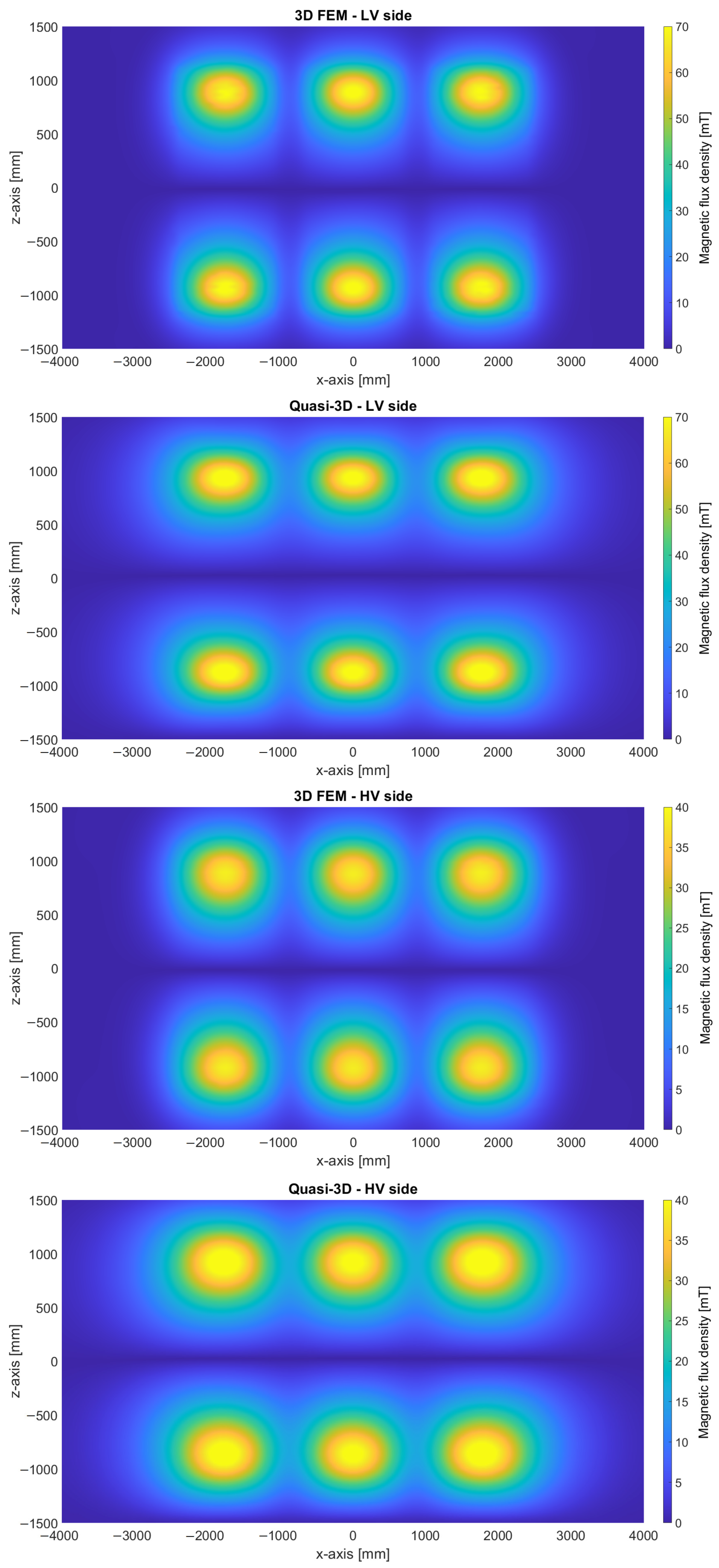
The distribution of the magnetic flux density in the vicinity of the tank shields		LV	5.0
		HV	7.7
The distribution of the magnetic flux density within the shield	Planar 2D FEM	LV	22.3
		HV	24.8
	Axisymmetric 2D FEM	LV	12.2
		HV	10.0
	Multi-step approach	LV	6.0
		HV	9.5
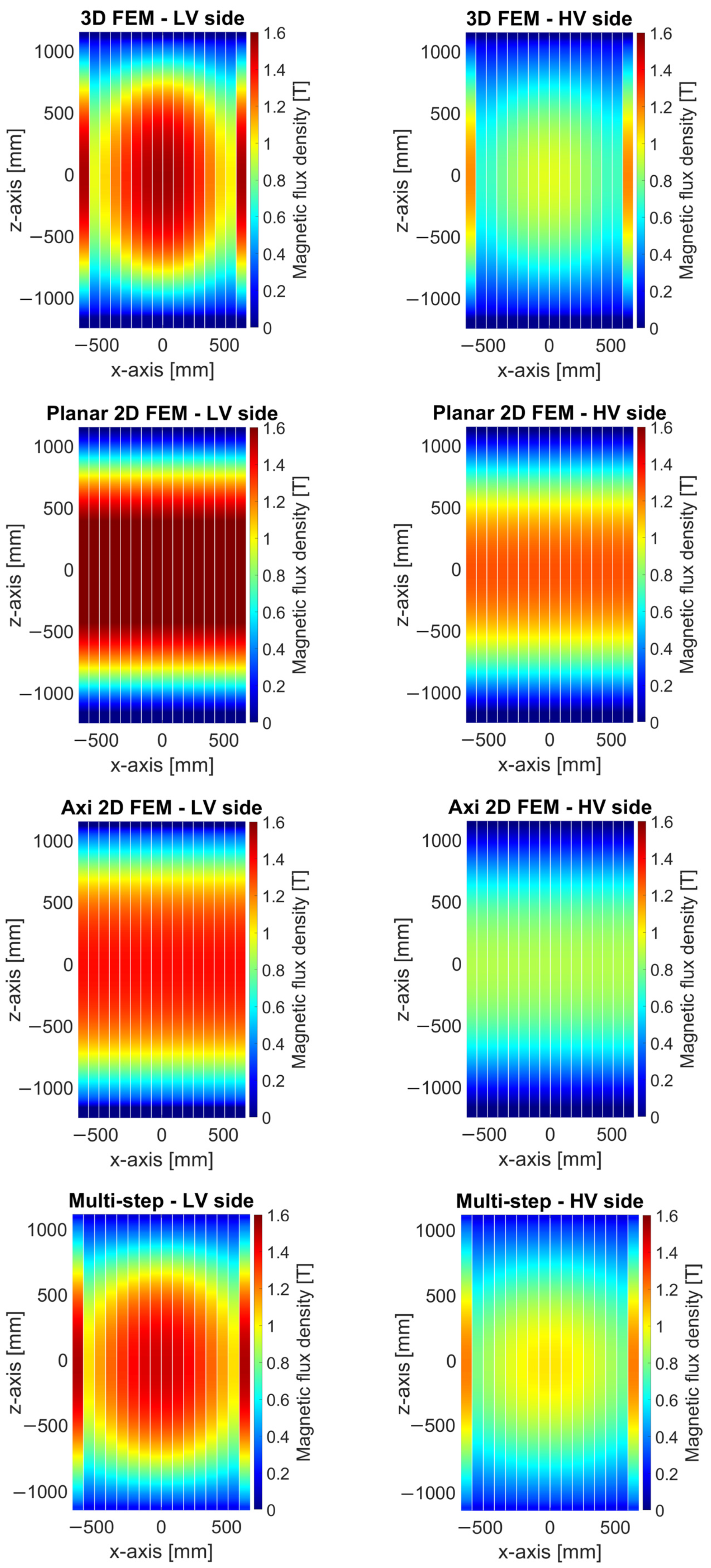
			2D FEM [T]	ε [%]
The maximum value of the magnetic flux density within the shield3D FEM:LV: 1.55 THV: 1.19 T	Planar 2D FEM	LV	1.76	14.0
		HV	1.27	7.0
	Axisymmetric 2D FEM	LV	1.38	−10.5
		HV	0.88	−26.2
	Multi-step approach	LV	1.52	−1.4
		HV	1.20	1.2

, whereas the computation time of all models is provided in

Table 3. Computation time.

Model	Time [min:s]	Time Reduction [%]
Planar 2D FEM	00:01	−99.97
Axisymmetric 2D FEM	00:01	−99.97
Multi-step approach	00:28	−99.19
3D FEM	57:32	0

.

5. Discussion

The results of the 2D FEM calculations are compared against those of the 3D FEM calculations. When comparing the maximum values of the magnetic flux density within the tank shield, which are calculated using the 2D FEM and the 3D FEM, it is shown that the highest relative error values for the planar and axisymmetric 2D FEM models are 14% and −26%, respectively, while the relative error for the multi-step approach is −1.4%. These results demonstrate that the multi-step approach is more accurate than both the planar and the axisymmetric 2D FEM models. Additionally, the multi-step approach can calculate the magnetic flux density in the horizontal direction (x-direction). When comparing the 2D distribution of the magnetic flux density within the tank shield, which is calculated using the 2D FEM and the 3D FEM, it is shown that the highest NRMSE values for the planar and axisymmetric 2D FEM models are 25% and 12%, respectively, while the NRMSE for the multi-step approach is 9.5%. The 3D FEM results show that the flux density non-uniformity in the horizontal direction is not negligible.

The computation time of the FEM models is also compared. The computation time of the 3D FEM model is ~1 h. The computation time of the planar and axisymmetric models is ~1 s, whereas the computation time of the multi-step approach is ~30 s. The difference between the computation times of the single 2D FEM models and the multi-step approach is negligibly small compared to the 3D FEM computation time.

6. Conclusions

A multi-step approach for the calculation of the magnetic flux density in the power transformer tank shields is proposed. The magnetic flux density is calculated in several steps using 2D FEM models with different cross-sections. The proposed approach can be an alternative to the well-established 3D FEM when a fast calculation is needed, e.g., during the transformer design phase.

The proposed approach can be easily implemented in the transformer design process. By automating the calculation steps, i.e., the 2D FEM calculations, a useful tool for optimizing the tank shield geometry can be obtained. Another possibility that the usually used 2D FEM models do not have is the calculation of the horizontal field distribution and optimization in a horizontal direction. This can lead to the more effective use of the tank shield material or a reduction in material costs. As such, the proposed approach has industrial value.

References

- Olivares-Galván, J.C.; Georgilakis, P.S.; Ocon-Valdez, R. A Review of Transformer Losses. Electr. Power Compon. Syst. 2009, 37, 1046–1062. [Google Scholar] [CrossRef]
- Kassi, K.S.; Fofana, I.; Meghnefi, F.; Yeo, Z. Impact of local overheating on conventional and hybrid insulations for power transformers. IEEE Trans. Dielectr. Electr. Insul. 2015, 22, 2543–2553. [Google Scholar] [CrossRef]
- Song, Z.; Wang, Y.; Mou, S.; Wu, Z.; Zhu, Y.; Xiang, B.; Zhou, C. Tank losses and magnetic shunts in a three phase power transformer. In Proceedings of the 2011 International Conference on Electrical Machines and Systems, Beijing, China, 20–23 August 2011; pp. 1–4. [Google Scholar] [CrossRef]
- Li, L.; Fu, W.N.; Ho, S.L.; Niu, S.; Li, Y. Numerical Analysis and Optimization of Lobe-Type Magnetic Shielding in a 334 MVA Single-Phase Auto-Transformer. IEEE Trans. Magn. 2014, 50, 1–4. [Google Scholar] [CrossRef]
- Yongbin, C.; Junyou, Y.; Hainian, Y.; Renyuan, T. Study on eddy current losses and shielding measures in large power transformers. IEEE Trans. Magn. 1994, 30, 3068–3071. [Google Scholar] [CrossRef]
- Moghaddami, M.; Sarwat, A.I.; de Leon, F. Reduction of Stray Loss in Power Transformers Using Horizontal Magnetic Wall Shunts. IEEE Trans. Magn. 2017, 53, 1–7. [Google Scholar] [CrossRef]
- Dasara, S.; Mishra, V.P. Shielding measures of power transformer to mitigate stray loss and hot spot through coupled 3D FEA. High Volt. 2017, 2, 267–273. [Google Scholar] [CrossRef]
- Al-Abadi, A.; Gamil, A.; Schatzl, F. Optimization of Magnetic Shunts Towards Efficient and Economical Power Transformers Design. In Proceedings of the 21st International Symposium on High Voltage Engineering, ISH 2019, Budapest, Hungary, 26–30 August 2019; Lecture Notes in Electrical Engineering. Springer: Cham, Switzerland, 2020; pp. 15–26. [Google Scholar] [CrossRef]
- Tsili, M.A.; Kladas, A.G.; Georgilakis, P.S.; Souflaris, A.T.; Paparigas, D.G. Geometry optimization of magnetic shunts in power transformers based on a particular hybrid finite-element boundary-element model and sensitivity analysis. IEEE Trans. Magn. 2005, 41, 1776–1779. [Google Scholar] [CrossRef]
- Hernandez, C.; Arjona, M.A.; Sturgess, J.P. Optimal Placement of a Wall-Tank Magnetic Shunt in a Transformer Using FE Models and a Stochastic-Deterministic Approach. In Proceedings of the 2006 12th Biennial IEEE Conference on Electromagnetic Field Computation, Miami, FL, USA, 30 April–3 May 2006; p. 468. [Google Scholar] [CrossRef]
- Jurković, Z.; Jurišić, B.; Župan, T. Multi-step approach for fast calculation of magnetic field in power transformer yoke shunt. Electr. Power Syst. Res. 2023, 221, 109407. [Google Scholar] [CrossRef]
- Jurković, Z.; Jurišić, B.; Župan, T. Fast Hybrid Approach for Calculation of Losses in Outer Packages of Transformer Core due to Perpendicular Stray Flux. IEEE Trans. Magn. 2021, 57, 1–4. [Google Scholar] [CrossRef]
- Liu, C.; Ruan, J.; Wen, W.; Gong, R.; Liao, C. Temperature rise of a dry-type transformer with quasi-3D coupled-field method. IET Electr. Power Appl. 2016, 10, 598–603. [Google Scholar] [CrossRef]
- Schlesinger, R.; Ewald, T.; Biela, J. Analytical Hybrid Quasi-3D Transformer Leakage Inductance Model. IEEE Trans Power Electron. 2023, 38, 5092–5106. [Google Scholar] [CrossRef]
- Jurković, M.; Žarko, D. Core-type transformer short-circuit voltage calculation using conformal mapping. IET Electr. Power Appl. 2020, 14, 2422–2430. [Google Scholar] [CrossRef]
- Jurković, M.; Žarko, D. Calculation of current distribution in parallel-connected transformer winding sections in the case of asymmetric magnetic field during short-circuit test. Electr. Power Syst. Res. 2022, 210, 108141. [Google Scholar] [CrossRef]
- Zhao, H.; Chau, K.T.; Yang, T.; Song, Z.; Liu, C. A Novel Quasi-3D Analytical Model for Axial Flux Motors Considering Magnetic Saturation. IEEE Trans. Energy Convers. 2022, 37, 1358–1368. [Google Scholar] [CrossRef]
- Rostami, N.; Rostami, M. Analysis of AFPM machines with cylindrically shaped magnets using quasi-3D method. COMPEL Int. J. Comput. Math. Electr. Electron. Eng. 2017, 36, 1168–1183. [Google Scholar] [CrossRef]
- Lv, G.; Zhou, T.; Zeng, D. Quasi-3D Analytic Method of the Single-Sided Linear Induction Motor With the Ladder Secondary. IEEE Trans. Ind. Electron. 2021, 68, 11817–11825. [Google Scholar] [CrossRef]
- Hemeida, A.; Lehikoinen, A.; Rasilo, P.; Vansompel, H.; Belahcen, A.; Arkkio, A.; Sergeant, P. A Simple and Efficient Quasi-3D Magnetic Equivalent Circuit for Surface Axial Flux Permanent Magnet Synchronous Machines. IEEE Trans. Ind. Electron. 2019, 66, 8318–8333. [Google Scholar] [CrossRef]
- Wen, X.; Yao, R.; Tegopoulos, J.A. Calculation of forces on the stator end windings of turbogenerator by the transient quasi-3D method. IEEE Trans. Magn. 1996, 32, 1669–1672. [Google Scholar] [CrossRef]
- Kulkarni, S.V.; Khaparde, S.A. Transformer Engineering, 2nd ed.; CRC Press: Boca Raton, FL, USA, 2017. [Google Scholar] [CrossRef]
- Meeker, D. Finite Element Method Magnetics, Version 4.2. Available online: https://www.femm.info (accessed on 5 September 2023).
- Van Bladel, J. Magnetostatic Fields at an Iron-Air Boundary. Am. J. Phys. 1961, 29, 732–736. [Google Scholar] [CrossRef]
- Yuferev, S.; Ida, N. Selection of the surface impedance boundary conditions for a given problem. IEEE Trans. Magn. 1999, 35, 1486–1489. [Google Scholar] [CrossRef]
- Lambert, M.; Sirois, F.; Martinez-Duro, M.; Mahseredjian, J. Analytical Calculation of Leakage Inductance for Low-Frequency Transformer Modeling. IEEE Trans. Power Deliv. 2013, 28, 507–515. [Google Scholar] [CrossRef]
- Moghaddami, M.; Moghadasi, A.; Sarwat, A.I. An algorithm for fast calculation of short circuit forces in high current busbars of electric arc furnace transformers based on method of images. Electr. Power Syst. Res. 2016, 136, 173–180. [Google Scholar] [CrossRef]