Abstract
Predictive modeling is important for assessing and reducing energy consumption and CO2 emissions of light-duty vehicles (LDVs). However, LDV emission datasets have not been fully analyzed, and the rich features of the data pose challenges in prediction. This study aims to conduct a comprehensive analysis of the CO2 emission data for LDVs and investigate key prediction model characteristics for the data. Vehicle features in the data are analyzed for their correlations and impact on emissions and fuel consumption. Linear and non-linear models with feature selection are assessed for accuracy and consistency in prediction. The main behaviors of the predictive models are analyzed with respect to vehicle data. The results show that the linear models can achieve good prediction performance comparable to that of nonlinear models and provide superior interpretability and reliability. The non-linear generalized additive models exhibit enhanced accuracy but display varying performance with model and parameter choices. The results verify the strong impact of fuel consumption and powertrain attributes on emissions and their substantial influence on the prediction models. The paper uncovers crucial relationships between vehicle features and CO2 emissions from LDVs. These findings provide insights for model and parameter selections for effective and reliable prediction of vehicle emissions and fuel consumption.
1. Introduction
Accurately assessing carbon dioxide (CO2) emissions from light-duty vehicles (LDVs) is a crucial precursor to carbon footprint reduction [1]. Global concerns regarding climate change have led to increased efforts to mitigate the impacts of greenhouse gas (GHG) emissions. One of the heavy contributors to GHG emissions is the CO2 released in transportation, particularly from LDVs [2,3]. Thus, emission reduction in operating various LDVs is a critical issue for sustainability. Effective strategies for emission reduction require CO2 emissions to be correctly evaluated for LDVs [1].
Predictive modeling is an indispensable and useful tool for assessing GHG emissions from LDVs [4]. The information on fuel consumption and resulting CO2 emissions has been measured and calculated for vehicles entering the market and has been made public by regulations. However, the published emission and energy values may not agree with actual ones, because they are usually based on measurements in a laboratory setting using standardized vehicle-operation profiles. Moreover, these measurement-based values cannot be available for future vehicles in forecasting because they are not produced and tested yet. Thus, useful prediction methods are necessary to evaluate GHG emission information based on vehicle specifications.
However, feature-rich vehicle datasets impose challenges in capturing the key relationships within the data for predictive modeling on vehicle GHG emissions and fuel consumption. As vehicle datasets become large and multifaceted, traditional modeling approaches may have difficulty identifying relevant patterns and interactions among variables. This difficulty is particularly severe when predicting CO2 emissions from LDVs, in which multiple vehicle characteristics contribute to emissions. Conventional straightforward prediction models offer simplicity but may struggle to capture subtle but important non-linear effects of vehicle features. While non-linear methods can capture intricate relationships with inherent flexibility, they may be susceptible to overfitting and the nonlinear effect of vehicle characteristics are not easy to interpret.
Hence, a systematic approach is desirable for effective feature selection, dimensionality reduction, and proper model selection to address the challenge of predicting CO2 emissions from feature-rich datasets in light-duty vehicles. One area of investigation is the effectiveness of linear and non-linear modeling techniques, given the complexities introduced by numerous vehicle features. A comparative evaluation of two well-known methodologies—linear model selection and non-linear methods—will be useful for examining the performance and efficiency of extracting meaningful relationships from feature-rich vehicle datasets. Another area of interest is the selection of features to be included in the prediction models. Appropriate feature selection would increase prediction efficiency and prevent overfitting.
The objective of this study is threefold: (1) an investigation of features affecting emissions, (2) an evaluation of linear and non-linear model performance, and (3) an analysis of prediction model behaviors. The first objective of this research is to perform a comprehensive analysis of the data on the CO2 emissions from LDVs. The relation of vehicle features to CO2 emissions and fuel consumption is investigated, and the relationships among the features are also examined. Second, this study aims to evaluate the performance of linear and non-linear models in predicting CO2 emissions from LDVs. A hypothesis test is conducted to evaluate the statistical significance of model parameters. These prediction models are compared in terms of accuracy and consistency. Third, this research aims to analyze the characteristics of the prediction models in diverse aspects. The linear models augmented by feature selection and regularization techniques are examined for model complexity and interpretability. Non-linear models, including generalized additive models (GAMs), are also analyzed for model complexity and interpretability.
The contributions of this study include uncovering vehicle feature relationships, assessing the effectiveness of linear and non-linear models with feature selection, and evaluating model reliability for CO2 emission prediction for LDVs. This study finds that models not using fuel consumption information still achieve consistently high accuracy with low uncertainty. The results indicate that a linear model with a proper subset selection yields performance close to non-linear models, demonstrating the validity of linear relations for proper trade-offs between model flexibility and interpretability. The analysis also reveals the importance of powertrain features in forecasting. The results also indicate that nonlinear models can capture the intricate relationships among variables, enabling more accurate estimation of CO2 emissions. These results can guide researchers and policymakers in choosing appropriate predictive models with optimized feature selection for emission estimation. These findings can advance informed decision-making in sustainable transportation planning, and support mitigating the environmental impact of vehicular emissions.
The remainder of this paper is structured as follows. Section 2 offers an overview of the relevant literature. Section 3 presents dataset characteristics and prediction modeling approaches. Section 4 analyzes and discusses the empirical results and suggests insights from the results. Section 5 concludes the paper.
2. Literature Review
Extensive research has been conducted to predict CO2 emissions and related energy use. These studies have utilized various modeling methods, including linear regression [5,6], support vector machines [7], and artificial neural networks [8]. Each method brings its strengths and limitations, depending on each prediction task. However, only a limited number of studies have focused on the prediction of CO2 emissions from LDVs.
As the cornerstone of modern science and engineering, data analysis aids decision-making across industries [9]. Current data analysis can handle complex data and utilizes advanced statistical methods to enhance accuracy and interpretability [9,10]. Emerging technologies such as artificial intelligence are pushing the boundaries of data analysis. In particular, data analysis has provided predictive insights and unlocked the potential of data to forecast future outcomes.
Among the various approaches, linear regression has been widely used in data analysis owing to its simplicity, interpretability, and well-established theoretical foundation [11,12]. Linear regression seeks to identify the best-fitting linear relationship between variables to make predictions [13]. In situations where the comprehension of straightforward relationships is essential, the linear models provide great interpretability [14].
Excluding irrelevant or less important variables from a multiple regression model is critical for model efficiency and interpretation of results. Numerous studies have incorporated feature selection techniques such as forward and backward selection in linear models [15,16] and have successfully improved model accuracy and removed irrelevant features. Advancements in regularization techniques, such as lasso [17] and ridge regression [18], have contributed to reducing overfitting and enhancing model generalization [19]. Thus, linear model selection can provide an effective framework for straightforward understanding of the impact of numerous factors on emissions. Feature selection can also aid in identifying key contributors to emissions and potential areas for reduction.
Non-linear models are often necessary when the key relationships among variables are much more complex than simple linear relations. These nonlinear models excel at uncovering complex non-linear patterns within the data and interactions among variables [14]. One such efficient non-linear method category includes GAMs. These models have been used increasingly in various scientific disciplines, including environmental science [20], epidemiology [21], and economics [22], owing to their ability to reveal intricate patterns possibly overlooked by linear models. GAMs flexibly provide smooth and continuous representations of non-linear patterns [23], making them potential candidates for exploring the complex relationships between vehicle features and CO2 emissions in LDVs to provide insights often missed by linear models. However, the complexity of GAMs can increase with choice of smoothing functions, possibly reducing the ease of interpretation and raising concerns about overfitting.
The balance between prediction accuracy and model interpretability is a critical consideration in predictive modeling [14]. Although advanced algorithms and intricate models often yield high forecasting accuracy, they may sacrifice the transparency and comprehensibility of underlying mechanisms. Achieving this trade-off is essential for CO2 emission prediction, as decision-makers and stakeholders require not only accurate emission assessments but also a clear understanding of the complex factors in emission sources. The prediction for LDV emissions is no exception in terms of the required accuracy and interpretability.
Various datasets exist regarding vehicular emissions. One of the comprehensive and systematically organized datasets is provided by the Canadian government for LDVs [24]. A few studies have analyzed this dataset using different methods, including polynomial regression with a single predictor and convolutional neural networks [25], as well as employing different machine learning methods [26]. Classification methods have been employed to predict CO2 ratings with high accuracy by incorporating fuel consumption as a primary feature [27].
It is necessary to develop emission prediction models without fuel consumption data and explore the effect of diverse vehicle characteristics. Studies on LDV emission data have used reported fuel consumption values in the dataset and obtained a straightforward relationship with emissions [27,28]. This indicates the intrinsic link between fuel consumption and CO2 emissions [28]. However, emission values may be converted from fuel consumption values. Moreover, exact information on fuel consumption may not always be readily available, severely constraining future emission predictions. Therefore, exploring alternative strategies is desirable for conditions in which fuel consumption data are not accessible.
Various tools and approaches exist for calculating and monitoring vehicle fuel consumption. In Europe, the New European Driving Cycle (NEDC) utilized standardized testing methods typically carried out in controlled laboratory settings to assess fuel efficiency in passenger cars [29]. In 2017, the World Harmonized Light Vehicles Test Procedure (WLTP) for LDVs was introduced to reflect real-world emission conditions [30]. The Vehicle Energy Consumption Calculation Tool (VECTO) is the European Commission’s simulation tool for calculating CO2 emissions and fuel consumption for heavy duty vehicles [31]. Japan has also adopted a standard for measuring power sources (fuel or electricity) from passenger cars under WLTP [32]. In the United States, the Environmental Protection Agency (EPA) provides standardized test methods and fuel consumption calculations for all new cars and light trucks [33]. Manufacturers in Canada employ standard five-cycle testing, involving controlled laboratory testing and analytical procedures, to generate fuel consumption data [34]. Several studies argue that, although inevitable, these standardized methods have limitations: they cannot reflect every aspect of numerous real-world conditions, and well-prepared standard testing can lead to misleading results [35,36,37]. Real time recording and metering are also used to promote reducing fuel consumption [37]. These measurement-based results, however, cannot be used to forecast future cars because they have not yet been created and assessed. Thus, appropriate prediction methods are required to assess GHG emission data based on vehicle specifications.
Although the prediction of vehicular energy use and CO2 emissions has been investigated extensively using various methods, there exist many aspects that still deserve more attention for better prediction. The trade-off between model flexibility and interpretability deserves more attention, in particular for best model selection. The selection of vehicle features also needs further investigation to improve models’ predictive power and interpretability. This study is conducted to address these research gaps in the existing literature. The contributions of this study include uncovering relationships among vehicle features, assessing the effectiveness of linear and non-linear models with best feature selection, and evaluating the reliability of the models for predicting CO2 emissions in LDVs.
3. Data and Methodology
This section describes data analysis and modeling approaches for predicting CO2 emissions from light duty vehicles (LDVs). The characteristics of the dataset used are provided, highlighting the relevance of key variables for evaluating CO2 emissions and energy use. This section also explains prediction models selected and compares their accuracy and efficiency.
3.1. Characteristics of the Data: Vehicle Features, Fuel Consumption, and CO2 Emissions
The dataset in this study contains fuel consumption and CO2 emission values from a variety of vehicles and their major features (specifications) in the LDV category. The dataset was collected from the official open data portal of the Canadian Government [24]. The data span a period of 10 years: from 2014 to 2023. LDVs are common vehicles of weight less than or equal to 10,000 pounds and used primarily for transporting passengers and cargo. LDVs include cars, vans, sport utility vehicles (SUVs), and pickup trucks. Therefore, the dataset can be considered comprehensive. The dataset covers most LDV types available in the North American market and provides sufficiently large data points for analysis. The dataset comprises 10,252 emission cases. Please note that the data are for new car models that are developed and introduced into the market with four- to seven-year intervals. For example, the same car names in the dataset may mean new car models of five years apart with different powertrains, specifications, and fuel consumptions; they cannot be considered as repeated measurements of the same car. Every new car model must receive a fuel consumption rating determined by mandatory standard testing [29,30,31,32,33,34].
The dataset contains diverse vehicle, fuel, and emission information. Table 1 shows summary statistics of the dataset regarding vehicle features and their corresponding values. The abbreviations and terms used in the table are explained in the Abbreviations. The dataset contains vehicle features, such as engine sizes, number of cylinders in engines, and number of gear ratios in transmissions (gearboxes), as well as fuel consumption data.

Table 1.
Summary of the carbon dioxide (CO2) emission values in the dataset.
The dataset consists of mixed data types. Categorical variables depict factor data types, allowing for the classification and comparison of discrete attributes. Numerical data types are employed to express non-categorical attributes, such as fuel consumption and number of engine cylinders. This information allows the analysis of the relationships between different vehicle features and CO2 emissions. CO2 emission values are in grams per kilometer (g/km).
The dataset includes fuel consumption values. Data on the amount of fuel consumption provide benefits for predicting CO2 emissions but also have limitations. In many countries, reporting and labeling of vehicle fuel efficiency for new cars have been mandatory. The amount of GHG emissions should also be reported. This fuel consumption information can be used to estimate CO2 emissions. However, this benefit is limited to existing vehicles on the market. For the prediction for future cars, the fuel consumption values are not available. The official fuel consumption values are also usually generated by laboratory testing with standardized operation profiles. Thus, there are situations in which we need to predict emissions without fuel consumption information and examine prediction performance.
3.2. Preprocessing of the Data
Given the mixed variable types within the vehicle dataset and the format of the input data types in prediction models, data preprocessing was necessary. This step was essential to enhance data quality, resolve inconsistencies, and ensure compatibility with the analytical methods to be used. The preprocessing steps included variable removal, data cleaning, data transformation, and normalization.
As the first step of data preprocessing, we excluded Make, Model, and Class from the considered features in predicting CO2 emissions. They were removed because of their categorical nature and the potential to introduce a high degree of complexity to the model. This step was similar to a data transformation phase during data preprocessing. These attributes involved various levels of categorization, such as different vehicle manufacturers, models, and classes. While these features can be influential in understanding the context of the data and the vehicles being analyzed, they might not directly contribute to the predictive accuracy for CO2 emissions based on vehicle specifications. By excluding them, the analysis could focus more on general attributes that have a direct and quantifiable relationship with CO2 emissions, potentially leading to a more streamlined and generalized predictive model.
As a next step of the preprocessing, a data cleaning process was also implemented to correct inaccuracies, outliers, and missing values. In this study, the tested dataset does not have any missing values.
Data transformation was also performed. In this study, the Gear variable was derived from the Transmission feature, representing the number of gear ratios (an integer). Then, the feature Transmission was removed from the dataset. In addition, since the Fuel feature was qualitative, binary variables were formulated for each fuel type: ethanol as type E, Diesel as type D, and gasoline as types X and Z.
Subsequently, the data underwent normalization or standardization to harmonize variables onto a common scale. This allowed for fair comparisons and prevented any undue influence of variable magnitudes on the analysis.
3.3. Exploratory Analysis of the Data
Before the main statistical modeling or hypothesis testing, preliminary exploratory data analysis (EDA) was conducted. EDA, including visual exploration of the data, helped to gain insights, identify patterns, and detect anomalies. It also served as a valuable tool for guiding feature selection processes.
The first EDA was a correlation analysis. A correlation analysis was conducted among seven quantitative feature variables: Gear (number of gear ratios in transmissions), Engine (engine size as the total volume of the combustion cylinders), Cylinder (number of cylinders in an engine), three Cons.* variables (fuel consumptions under three operating conditions), and CO2 Emissions. Figure 1 shows the pairwise correlations between different quantitative feature variables in the dataset. The number in each cell (square) is the linear correlation coefficient between the two variables, which ranges from −1 to 1.
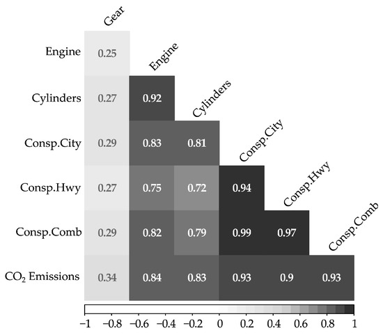
Figure 1.
Correlation matrix of quantitative variables.
As shown in Figure 1, all seven features are positively correlated. The Engine and Cylinders features have a strong positive correlation (0.92), suggesting that larger engine sizes are often associated with more cylinders. The correlation coefficient between Engine and Consp.City (fuel consumption in city) is 0.83, another strong association indicating larger engines consume more fuel. There is a relatively weak correlation between Gear and the other variables. CO2 Emissions have moderate to strong positive correlations with Engine, Cylinders, and Fuel consumptions variables. This means that these attributes are potentially influential factors affecting CO2 emissions in LDVs, but a single feature may not be able to fully explain CO2 emissions. Fuel consumption variables have extraordinarily strong correlations with CO2 emissions, as expected. As revealed by data analysis in later sections, fuel consumption and CO2 emissions can be proxies for each other in prediction models.
The strong relationship between the engine size and number of cylinders is elaborated in Figure 2. As indicated in Figure 2a, as the engine size increases, so does the number of cylinders. This trend reflects that more combustion chambers are required to accommodate larger total engine displacement (volume). This strong correlation suggests a possibility to include either the engine size or number of cylinders in a predictive model for CO2 emissions, rather than both, if we would like to reduce model complexity.
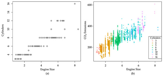
Figure 2.
Relationship between variables. (a) The engine size and number of cylinders. (b) CO2 emissions and the engine size segregated by the number of cylinders.
The exploratory analysis shown in Figure 2a also revealed some minor cases with special vehicle characteristics. One example is an exceptionally large engine size of over seven liters. There exist two such cases that look like outliers. In fact, these vehicles are luxury sports car models: Bugatti Chiron with a 16-cylinder 8-liter engine and Dodge Viper with a 10-cylinder 8.4-liter engine. These outliers representing muscle cars may affect the results of the statistical analysis, and this effect will be examined in later sections.
Figure 2b reveals the relationship between CO2 emissions and engine size, segregated by the number of cylinders. There is a general trend upward in each group of cylinders. This trend suggests that vehicles with larger engine sizes within the same cylinder category tend to emit more CO2. It is known that a greater number of cylinders typically allows for a larger total combustion volume, namely a larger engine size. In this way, we can explore a potential causal relationship between vehicle features and emission values.
Each of the engine sizes and number of cylinders has a consistently strong correlation with CO2 emissions regardless of time (vehicle model year or emission assessment year). Figure 3 illustrates the average CO2 emissions over a span of 10 years, from 2014 to 2023. The emission values are stratified by the engine size and number of cylinders regardless of time changes. While there is a slight upward trend in emissions over time, the increase is not substantial. Thus, we may consider excluding the year variable in features selection since it appears to have a relatively minor impact on the emission pattern.
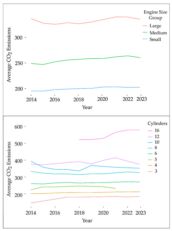
Figure 3.
Average CO2 emissions by engine size (top figure) and number of cylinders (bottom figure) over time.
In the top panel of Figure 3, the engine sizes were categorized into three groups: small (≤2), medium (2–4), and large (4–8.4). The larger the engine size, the higher the CO2 emissions. The emissions of the medium engine group were approximately 50 g/km higher than those of the small group. The large engine group had approximately 70 g/km more emissions than the medium group. The average emissions of the large engine group had slightly more fluctuations over time.
The bottom panel of Figure 3 shows the average CO2 emissions over time based on the number of cylinders. Eight values in cylinder sizes were used in the dataset. Cylinders 5 and 16 appeared only for part of the entire time frame, reflecting rare cases in the market or recent introductions (size 16 began in 2018). The 16-cylinder case had the highest emissions, exceeding 500 g/km, whereas the other cases consistently recorded below 400 g/km. For fewer than eight cylinders, the average CO2 emissions remained relatively stable over time, whereas cylinders exceeding 10 exhibited more fluctuations. The trend fluctuation is not unusual, with only a few data points for the very high number of cylinders. As mentioned previously, a small number of these data points correspond to a few sports car models.
3.4. Modeling Approaches and Evaluation Metrics
In this study, the choice of an appropriate model hinges on a key trade-off between model flexibility and interpretability. Linear models offer a high degree of interpretability, making them easier to comprehend the relationships between variables. However, their simplicity may limit the ability to capture the complex and non-linear patterns inherent in data, potentially compromising predictive power. On the other hand, many non-linear models can capture intricate relationships among data features. However, non-linear models are prone to overfitting and difficult to interpret.
Some methods provide a middle ground, offering greater flexibility than simple linear models but still preserving a degree of interpretability. For instance, generalized additive models (GAMs) can capture complex non-linear relationships in the data using a smoothing function. This makes GAMs a valuable tool for understanding intricate patterns. However, it is worth noting that the complexity of GAMs can increase with the number of features and the choice of smoothing or segmentation strategies. This added complexity can sometimes reduce interpretability.
Recognizing the importance of this trade-off, this study employs diverse models, ranging from linear methods for their interpretability to non-linear methods like GAMs for their enhanced flexibility. By systematically adjusting model complexities and fine-tuning parameter settings, this research aims to reveal valuable insights into striking the optimal balance between predictive accuracy and interpretability for the emission dataset. Through this exploration, we aim to identify the most suitable modeling strategy for effectively addressing the core patterns and relationships within the data.
This study also uses feature selection for refined and efficient predictive models. Feature selection chooses subsets of variables from a larger pool of variables to construct more efficient and meaningful models. In particular, feature selection is used for linear models in this study because it allows for the identification of the most influential variables in predicting CO2 emissions, helps enhance interpretability, and reduces overfitting. In feature selection, two scenarios are considered, depending on the use of fuel consumption features. In the first scenario, the fuel consumption-related features (Consp.City, Consp.Hwy, and Consp.Comb) are included in the prediction model. The second scenario assumes that fuel consumption data are not available, and the fuel consumption-related features are excluded from the variables in the prediction model. Furthermore, interaction terms between features were incorporated into the models; however, their presentation is omitted in this paper due to the page limit.
To evaluate the statistical significance of model parameters, a hypothesis test is also conducted to examine the null hypothesis of:
H0:
There is no relationship between the predictor variable and response (CO2 emissions); model coefficient .
Ha:
There is some relationship between the predictor variable and response (CO2 emissions); model coefficient .
3.4.1. Linear Regression Methods
The linear models in this study are distinguished by the features included in each model. Various subset selection methods are employed to fit the linear models to the emission data. Each linear model selects a different subset of features among 10 vehicle features to construct its predictive model. The linear models are divided into two categories depending on the inclusion of fuel consumption information in the selected feature subset; one uses fuel consumption variables to fit the model, but the other does not. In each category, more linear models are examined by further feature selection.
In this study, feature selection utilizes several methods, including best subset selection, validation set approach, and lasso. The best model among a set of models of different sizes can be determined by choosing the one with the highest adjusted R2 or lowest Bayesian information criterion (BIC) and Akaike information criterion (AIC). These techniques help strike a balance between model complexity and prediction performance. The objective is to avoid overfitting by excluding irrelevant or redundant variables while ensuring that the model captures essential patterns in the data. EDA and correlation analysis also serve as a starting point for feature selection in the linear regression model. They verify that only relevant variables are incorporated in the models.
3.4.2. Non-Linear Methods
In this study, we employ GAMs to capture possible intricate non-linear relationship between predictor and response variables (CO2 emissions). GAMs offer a general framework for extending conventional linear models by accommodating non-linear functions, denoted as fj for variable j. These non-linear functions are systematically computed for each feature, and their contributions are then combined to form the overall model. In this study, these functions are fitted using smoothing splines due to their flexibility. The general form of GAMs is as follows (note that the mathematical symbols are explained in Abbreviations):
The selection of the degrees of freedom (df) in functions of GAMs is a deliberate process aimed at achieving a balance between model flexibility and avoiding overfitting. The degrees of freedom can be chosen through an iterative procedure. The models can be set to a conservative df value and then the df value is adjusted incrementally to observe changes in model fit and predictive accuracy.
In addition, the smoothing parameter λ for smoothing splines is fine-tuned using leave-one-out cross-validation (LOOCV). This approach helps identify the optimal value of λ, which determines the appropriate degrees of freedom. By using LOOCV, the model’s performance is assessed comprehensively. This ensures that the chosen values for λ and df result in a GAM that effectively captures essential patterns in the data, avoiding overfitting.
3.4.3. Evaluation Metrics
The accuracy of the models is evaluated by three metrics. They are the mean squared error (MSE), root mean squared error (RMSE), and coefficient of determination (R2):
A low MSE and RMSE or high R2 values generally indicate better model performance. The RMSE effectively represents the average difference between the predicted and observed CO2 emissions values.
In addition to the three metrics, additional measures are evaluated. To examine the performance consistency of the model selection, the uncertainty of the evaluation metrics is also assessed. The uncertainty of evaluation metrics is evaluated using Monte Carlo cross-validation (MCCV) or repeated random subsampling. MCCV is a straightforward method that randomly divides the data into two parts (learning and test sets) and repeats the procedure N times [38]. In this study, 500 different train-test sets are used (N = 500). In each of the 500 train-test split cases, the data are randomly divided into a 70% training and 30% test set.
The standard deviation (SD) among these different test sets serves as an indicator of the degree of uncertainty in estimating the aforementioned metrics. The SD of the metrics for the 500 cases represents the variability in these metrics for each prediction model. This variability measure can be considered as standard error (SE) [14,39]. These uncertainties can provide a range of values around the average statistics (MSE, RMSE, and R2), and suggest the level of confidence on the estimates or variability among them. Low SD values indicate performance consistency regardless of case changes; high SD values suggest less performance consistency with changes in cases.
4. Results, Analysis, and Discussion
This section presents the results obtained from linear and non-linear prediction models. The empirical results are also analyzed in terms of model performance and characteristics. The practical implications are also discussed.
The computational resources for this study were not demanding. The learning models were implemented on a computation server with an Intel Xeon Silver 4210 CPU at 2.20 GHz and 96.0 GB of RAM, utilizing R Studio. The execution times for the models were not usually long.
4.1. Linear Regression Models
The results of a variety of linear regression models were examined, and the analysis shows that the linear models predict emission values consistently with high accuracy and effectiveness as well as provide excellent interpretability and reliability. The results are summarized in Table 2. These linear regression models, though less flexible than non-linear counterparts, are able to predict emissions with high accuracy. To evaluate the statistical significance of model parameters, a hypothesis test is also conducted to examine the null hypothesis that the coefficient for a particular variable is equal to zero, against the alternative hypothesis that it is not equal to zero. The coefficients of the models have low p-values, indicating statistical significance. Thus, we can reject the null hypothesis. In other words, we assert the presence of a relationship between predictor variable and the response CO2 emissions, denoted by model coefficient . A comprehensive analysis of different linear models was conducted with 500 different train-test splits in MCCV, and the analysis shows the consistency of the linear models in predicting CO2 emissions against the varying train-test sets. The SD values are within 3% of the average values. The linear models also provide high interpretability through linear variable relations such as additivity and proportionality.
Table 2.
Performance comparison of linear models with different subset selection. (Note that the ‘✓’ mark indicates the inclusion of the corresponding predictor variable.).
In general, the models in the first scenario using the fuel consumption data exhibit superior average performance with lower variability, compared with the models in the second scenario not using the fuel consumption data. The study explored the predictive power of linear models with the scenarios involving the presence or absence of fuel consumption data. In scenarios where fuel consumption data are unavailable, the fuel consumption-related features (Consp.City, Consp.Hwy, and Consp.Comb) are excluded, indicated by the shaded columns in Table 2. The predictive performance of linear models is considerably high with the fuel consumption data. For example, with the fuel consumption data, the R2 values are close to one; without the fuel consumption data, the R2 is still high, ranging from 0.7 to 0.8.
The strong influence of the fuel consumption data is more noticeable with feature selection in the model construction. In Table 2, when fuel consumption data are available, there are two models. The base linear regression model includes all 10 features, and the model with subset selection relies solely on three features—combined fuel consumption, and fuel types D and E. The model with subset selection yields minimal difference from the base linear regression model in terms of average MSE, RMSE, and R2. With superior values in MSE (approximately 28) and R2 (approximately 0.99) and only marginal differences from the base model, choosing models with fewer feature sets can enhance interpretability. The low SD of the metrics indicates less variability in the respective measures.
Note that the strong influence of the fuel consumption data may originate from the way the emission data are generated in the provided dataset. The CO2 emission values in the original government data were deduced from the fuel consumption values possibly through simple conversion (calculation) rather than the direct emission measurements on vehicles. This is speculated due to the evident relationship between CO2 emissions and fuel consumption, making it feasible to predict either of these variables with a similar level of accuracy. This means that only one of the variables is sufficient for prediction models and the other variable can be derived by simple conversion. Thus, we can also predict fuel consumption and obtain emissions through conversion.
In the second scenario in which the fuel consumption data are not available, the linear regression models still predict the emissions quite accurately. These linear models mostly utilize the powertrain features (first three variables in Table 2) and exclude certain binary fuel variables. The R2 values are over 0.7, with only general vehicle characteristics such as powertrain specifications.
In addition, even in the scenario of unavailable fuel consumption data, these linear methods predict emissions quite consistently. The SD for each of these metrics is calculated across 500 different train-test splits in MCCV, as shown on the right-hand side of Table 2. In most cases, the SD values fluctuate around 1% for R2, 1.5% for RMSE and 3% for MSE. These low SD values in the performance of each prediction model mean consistency regardless of train-test set changes.
The prediction is also consistent regardless of the linear models with different feature subsets. The results show quite similar performance metrics, indicated by slight differences in terms of average MSE, RMSE, and R2 across models. These linear models exhibit only minimal variations in performance metric averages. RMSE values are around 31 and R2 values around 0.74. In addition, the SD in each metric does not differ significantly between models.
As the performance metrics decline, variability tends to increase. For instance, considering the linear regression model, the RMSE’s SD in the scenario of available fuel consumption data is approximately 0.27, whereas it reaches 0.45 or 0.48 in that of unavailable fuel consumption data. Table 2 shows that in the cases of available fuel consumption data, 68% of the results in each model fall within a range of ±0.001 (one SD away from the mean), while in the other cases the range is wider at ±0.007.
The results of the feature selection indicate that the powertrain characteristics are reliable features for predicting CO2 emissions. Subset selection 1 includes only the powertrain features. It is worth noting that by deselecting the fuel-type variables, subset selection 1 demonstrates only slight differences compared with other linear methods that incorporate a larger number of variables. This suggests that the impact of fuel-type variables is not as strong as expected in terms of prediction model performance. The impact of fuel-type variables needs to be examined with additional data on vehicle characteristics in a separate future study.
Analysis of the feature selection results indicates that, among the powertrain characteristics, Engine Size is the most influential feature. Subset selections 2–4 were conducted to explore the relationship between Engine Size and Cylinders. The selections that include the Engine Size feature tend to yield slightly improved results compared to those that exclude it. For instance, the outcomes indicate that subset selection 4 achieves an R2 value of 0.72 ± 0.007 and an RMSE value of 31.85 ± 0.488 with just two variables (Gear and Engine Size). Subset selection 3, which includes four variables but excludes the Engine Size feature, achieves an R2 value of 0.71 ± 0.008 and RMSE value of 32.86 ± 0.484. A supplementary performance assessment of subset selection 4 is carried out using 80:20 train-test ratio for the splits. The results remain consistent with that of the earlier split ratio, yielding an R2 value of 0.72 ± 0.008 and RMSE of 31.85 ± 0.643.
An analysis of the sensitivity to outliers was conducted to assess the robustness of the selected predictors to subset selection 1. Outliers resembling those depicted in Figure 2 are omitted, and the result was compared with that of the original model. The p-values for all coefficients were less than 10−16, indicating statistical significance. Overall, both models provide statistically significant relationships between the predictors and CO2 emissions, with similar intercepts and coefficients for most predictors. The detailed results are omitted due to space constraints in the paper.
In addition, models incorporating interaction terms among features have been explored. On average, these models show around 1.6% increase in R2 compared to the models without interaction terms. The details are not described in this section due to their non-significance and page limit.
The results analysis demonstrates the effectiveness of feature selection of the models for the dataset. When linear models exhibit comparable performance metrics, opting for models with fewer variables provides enhanced interpretability without too much sacrificing of predictive accuracy. This streamlined approach not only simplifies the model but also facilitates a clearer understanding of the underlying relationships between vehicle attributes and CO2 emissions. By employing subset selection methods, analysts can navigate the challenge of feature-rich datasets, ensuring that the chosen variables contribute significantly to the model’s predictive power and interpretability. The combination of linear regression and subset selection methods offers a powerful toolkit for modeling and understanding relationships within complex datasets.
4.2. Non-Linear Regression Models
In this section, the results of non-linear models will be explored to examine how they enhance prediction. We will focus on the cases in which fuel consumption data are unavailable, thereby narrowing our analysis to seven key features for predicting CO2 emissions. Hence, not using the fuel consumption data is reasonable because an almost perfect linear relationship exists between emissions and fuel consumption, as shown in the preceding sections. Because of the relationship between the emission and fuel consumption data, instead of emissions, fuel consumption can be the response variable.
Among various non-linear methods, GAMs are employed to accommodate non-linear associations between individual vehicle features and the response variable (CO2 emissions). GAMs compute distinct non-linear functions for each feature and aggregate their contributions. Following Equation (1), the GAMs used to predict CO2 emissions are as follows:
Although Engine Size, Gear, and Cylinders are quantitative variables, Fuel Type is qualitative. In Equation (5), the first three functions f1 to f3 are modeled using smoothing splines for the quantitative variables. The fourth function f4 is established by assigning a distinct constant value for each fuel type.
Figure 4 presents the relationship between each feature and the response (CO2 emission), as well as the results of fitting the model by Equation (5) for different GAMs. Each segment in a sub-figure represents the fitted function alongside pointwise standard errors. All models in Figure 4 utilize a step function to model the fuel type.
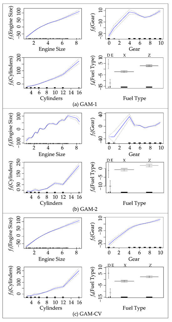
Figure 4.
The relationship between the response (CO2 emissions) and each selected feature in different GAMs.
Each model represents its unique configuration with different df for the Engine, Gear, and Cylinders features. In Figure 4a,b, both GAM-1 and GAM-2 are customized with pre-determined degrees of freedom for these specific features. GAM-2 has a higher df. Unlike these two models, GAM-CV in Figure 4c utilizes a LOOCV method to determine an appropriate df for each function. The specific df settings are listed in Table 3.
Table 3.
Average performance comparison of the GAMs with different degrees of freedom across 500 train-test splits.
Across all models in Figure 4, under the condition that all the other variables are held constant, each function reveals clear trends in CO2 emissions by each variable. The f1 (Engine Size) panel shows a significant increase in emissions with larger engines, attributed to the fact that larger engines typically burn more fuel. In the f2 (Gear) panel, emissions exhibit fluctuations but generally rise with higher gear values, indicating that higher gear number transmissions are associated with cars of more fuel consumption. The f3 (Cylinders) panel illustrates emissions increasing with more cylinders due to the greater capacity for combustion in engines with more cylinders. In the fuel type panel, CO2 emissions are lowest for ethanol (fuel type E) and high for the other types (diesel as fuel types D and gasoline as fuel types X and Z), reflecting differences in the energy density and combustion characteristics of the fuel types as well as different life cycle emissions [40].
Unlike the other models, GAM-2 offers a high degree of freedom with 17 degrees for Gear and Engine Size and 19 for Cylinders, resulting in more intricate and fluctuating functions as depicted in Figure 4b. In the engine function, emissions generally rise with larger engine sizes, peaking at size 7. The decline at Engine Size 8 may not be statistically meaningful; there are only a few such data points. The high df and limited number of data points may make the analysis biased, resulting in an inaccurate trend. In such a small number of cases, some unique vehicle characteristics may affect emission values, including large engines on relatively lightweight vehicles such as sport cars. As explained in Section 2, these are luxury muscle cars that may not seriously concern fuel consumption.
For both GAM-1 and GAM-2, the gear function panel shows a quite similar trend in CO2 emissions. The emissions increase up to gear size 4, followed by a decrease up to size 7, and then an increase. These patterns likely stem from various factors, including transmission efficiency, engine power output, and emission control technologies. The cases in which the number of gears is zero and one correspond to the vehicles with continuously variable transmissions (CVT) or only a few special vehicles with exceedingly small engines. They are abbreviated as AV0 and AV1 in the dataset. Some combinations of a CVT and engine can increase fuel efficiency. It is reasonable that the emissions decrease as the number of gears increases from four to six or eight. The transmissions in vehicles are usually more efficient with more available gear ratios. The higher numbers may also mean more recent and thus more fuel-efficient vehicles.
However, this trend of CO2 emissions with gear variable is worth more detailed attention. The increasing fuel efficiency with higher gear variable values does not seem always to be the case. The emission increase beyond number 7 may reflect several possibilities. In some cases, the transmissions with more available gear ratios may have counter-effects for overall fuel efficiency of a vehicle. A high number in available gear ratios may mean a large thus less fuel-efficient car. Overfitting problems may exist. In fact, in this dataset, this non-linear behavior is a consequence of the combination of a high degree of freedom of the GAMs and limited data points beyond variable value 7. The two data points correspond to fuel-guzzling sports cars as mentioned in Section 3.1. These outliers distorted the non-linear trend in GAM-1 and GAM-2.
Overall, GAM-2 excels in capturing intricate non-linear connections between each feature and emission responses, surpassing the capabilities of GAM-1. This enhanced flexibility may come at the cost of overfitting when applied to novel, unseen data.
To address this concern, GAM-CV is explored. Figure 4c illustrates the results of GAM-CV. This model employs a cross-validation approach to ascertain the optimal degrees of freedom for each function, setting them at 3, 2, and 8 for gear, engine, and cylinder variables, respectively. Although this cross-validation procedure slightly reduces predictive performance, it enhances the model’s generalization ability. Thus, GAM-CV ensures that the model is not overly tailored to the training data, allowing it to perform reliably and make accurate predictions on new, unseen data.
Table 3 presents the average performance metrics of the models depicted in Figure 4 over the 500 samples of train-test splits in MCCV. It shows that in 68% of the outcomes, GAM-2 exhibits slightly better performance, as indicated by its lower RMSE values, approximately 28.8 g/km (±0.435), and higher R2 values, approximately 0.77. On the other hand, GAM-CV shows a minor reduction in predictive performance with R2 values of roughly 0.76 (±0.007) and MSE value of approximately 897 (±25.9). However, it offers the advantage of preventing the model from overfitting to the training data.
4.3. Linear versus Non-Linear Models: Performance Variations and Insights
This section compares the results obtained from linear and non-linear methods for predicting CO2 emissions and evaluates the variations in models’ performance.
Both approaches have distinct characteristics that affect their predictive performance. Linear regression offers interpretability and simplicity, making it suitable for understanding the direct relationships between variables. However, the nonlinear method can capture complex relations within the data, accommodating non-linear patterns.
Figure 5 compares the performances of the various methods used to predict CO2 emissions without the fuel consumption data. The evaluation of these methods is based on the mean value of two performance metrics: RMSE and R2.
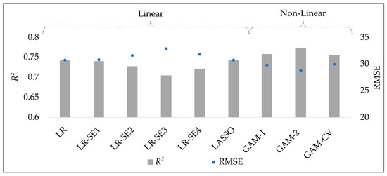
Figure 5.
Average performance comparison of different linear and non-linear methods.
In Figure 5, linear models exhibit slightly inferior performance compared to non-linear methods. The linear models achieve RMSE values of approximately 31 g/km and R2 values around 0.73. On the other hand, non-linear methods display higher R2 values: greater by two to seven percentage points. They also achieve lower RMSE values, averaging 3 g/km less compared with the linear approaches.
Among the non-linear methods, both GAM-1 and GAM-CV demonstrate substantial effectiveness, with only marginal differences in their performance. Both models attain an R2 value of approximately 0.76, with GAM-CV excelling in enhancing the model’s generalization ability through a lower degree of freedom setting. Despite their effectiveness, GAMs may present challenges in terms of interpretability. In contrast, a linear model LR-SE1 (linear regression with subset selection 1) provides greater interpretability and demonstrates a performance that is not significantly different from those of GAMs.
Figure 6 illustrates the consistency of the models’ performance over various (500) train-test splits in MCCV. The spreads of the performance over train-test splits are shown using box plots and histograms. Figure 6 compares three representative models: LR, LR-SE4, and GAM-CV. The base linear regression model LR (utilizing all features) demonstrates a moderate predictive ability with an RMSE of 30.7 ± 0.454 and an R2 of 0.74 ± 0.007. LR-SE4 (linear regression with subset selection 4) comprises only two features (gear and engine) and offers a more straightforward interpretation. In contrast, GAM-CV involves four features with non-linear functions and offers slightly higher performance compared to the other two models. However, this comes at a cost of added complexity in interpretation, making it considerably more complex to interpret.
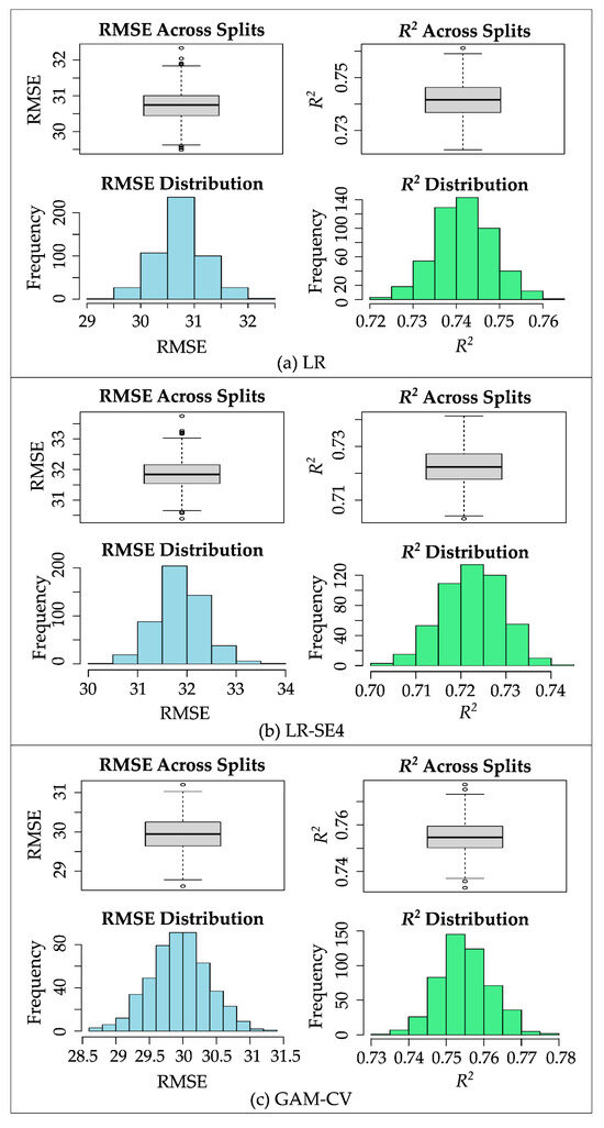
Figure 6.
Performance variation across 500 train-test splits in MCCV between different models.
While from a purely statistical point of view the difference between GAM-CV and LR-SE4 is significant, in a practical sense it remains relatively small. A paired t-test at the 95% confidence level indicates that the difference in RMSE and R2 between GAM-CV and LR-SE4 is statistically significant. This statistical significance is obvious, because one is a linear model and the other a non-linear one. However, in practice, this difference is relatively negligible: approximately 2 g/km and three percentage point differences in RMSE and R2, respectively.
For this dataset, linear models with subset selection yield reasonably superior results with interpretability. We can see that linear models offer a high degree of interpretability, making it easier to comprehend the relationships among variables. However, their simplicity may limit their ability to capture the complex and non-linear patterns inherent in some datasets, potentially compromising predictive power. On the other hand, non-linear methods like GAMs provide a greater level of flexibility than linear models, and still preserve a degree of interpretability. However, the complexity of GAMs can increase with the number of features and the choice of smoothing or segmentation strategies. This added complexity can sometimes reduce the ease of interpretation and raise concerns about overfitting. The decision between linear and non-linear methods necessitates a thoughtful consideration of these tradeoffs, including the risk of overfitting, to align with specific modeling objectives and the characteristics of the dataset.
4.4. Insights for Decision Making and Practice
The results of this study can provide significant implications in practice for predicting CO2 emissions and fuel consumption as well as sustainable planning in design, manufacturing, supply chains, etc. The study’s findings can offer valuable guidance for researchers, policymakers, and automotive manufacturers in their efforts to address sustainability challenges and reduce the carbon footprints of LDVs.
The results suggest that linear models can be used successfully in many practical situations such as forecasting for an industry or the transportation sector. The analysis showed that, despite their simplicity, linear models could predict CO2 emissions (or fuel consumption) with a comparable accuracy to that of nonlinear models. The linear models for emission prediction are also easy to implement in practice. They can be estimated using simple calculations and ordinary software such as spreadsheet software. The effects of the vehicle parameters in the linear models are also easy to interpret owing to their additivity and proportionality. These linear models are intuitive to understand and recognize the effect of each variable for practitioners. Thus, unless extremely high accuracy is necessary, linear models could be utilized easily and widely with confidence for many applications.
Successful prediction using parsimonious feature selection suggests the effectiveness of using only important vehicle variables for emission and energy use prediction in practice. The results showed that models with fewer variables could enhance interpretability without significantly compromising accuracy. For example, a linear model incorporating only Gear and Engine Size features produced satisfactory results while maintaining high interpretability. Applying feature selection intuitively using variable correlation could be an easy but effective approach in practice.
The results imply that the prediction models can be used for forecasting the emissions of future vehicles that do not have fuel consumption information yet. The results showed that the vehicle emissions can be estimated quite accurately using only vehicle specifications but fuel consumption values. The feature selection analysis emphasizes that, within powertrain characteristics, engine size is the most influential factor affecting CO2 emissions. These findings mean that the survey or market trends on vehicle specifications could be used effectively to forecast emission trends in the future. These overall forecasts can be utilized for the analysis of the vehicle market and transportation sector. These forecasts will also be useful for decision-makers in formulating policies and regulations for the future. Meaningful forecasts can help prepare effective strategies for emission reduction, contributing to an environmentally friendly transportation ecosystem.
The analysis of the model performance suggests enormous potential for improved accuracy with additional feature data and modified prediction models. Our research highlights the significance of tailoring predictive models based on the specific attributes in the dataset. Feature selection and regularization techniques play pivotal roles in augmenting the predictive capabilities of the prediction models. For example, the results indicated the importance of powertrain features in the prediction. By carefully selecting relevant features, practitioners can enhance prediction accuracy while maintaining model simplicity and interpretability. This accuracy can be enhanced further by augmenting other vehicle features such as vehicle weight and operational patterns. Moreover, a practitioner may combine such new data with the dataset of this study to improve forecasting.
With the new feature data, decision-makers can adopt one of the prediction models presented in this study. When faced with different data scenarios, decision-makers can choose appropriate modeling techniques to optimize the predictive performance. For example, the GAMs in this study can be used with additional features to improve accuracy. Feature selection techniques can still be used to examine for the best choice among the linear and non-linear prediction models.
The results also suggest that in practice highly non-linear models should be used with caution and the degrees of freedom should increase sparingly. In particular, a model with a high degree of freedom and limited data points can distort the analysis, as demonstrated by the high number of gear ratios in sports cars. More gear steps in transmissions are typically beneficial for reduced CO2 emissions, but this was not the case for sports cars. Therefore, nonlinear models could be prone to being biased. The limited data points should also be examined owing to their unique characteristics.
The findings also demonstrate that the choice between linear and nonlinear models depends on the trade-off between interpretability and complexity as well as the specific prediction task. In practice, linear models are suitable for many applications, unless highly precise predictions require the flexibility of non-linear approaches. Linear models, especially those with subset selection, deliver reasonable results with high interpretability. However, their simplicity may limit their ability to capture intricate non-linear patterns. In contrast, nonlinear models such as GAMs offer greater flexibility but may pose challenges in interpretation owing to their increased complexity.
The prediction methods used in this study can be applied to a variety of areas. For example, forecasting can be used for roughly estimating CO2 emissions during the initial design stages of vehicle development. Optimizing the engine design of a car can contribute to fuel consumption and CO2 emission reduction. The prediction methods can also play a key role in estimating the GHG emissions in the value chain of any organization. Accurate prediction is necessary for emission measurement and reporting direct Scope 1 and indirect Scope 3 (upstream and downstream in a supply chain) emissions. Accurate forecasting can also provide key data for planning effective emission reduction. These efforts can help governments and manufacturers to satisfy the total emission limits set by the increasingly stringent regulations worldwide.
5. Summary and Conclusions
This study conducted comprehensive analysis on the data of the CO2 emissions and fuel consumption from light-duty vehicles (LDVs) and investigated important characteristics of linear and non-linear prediction models. First, this study characterized the LDVs’ emission data and identified the key relations among vehicle features and emissions. Second, the study evaluated the performance of linear and non-linear models in forecasting CO2 emissions from LDVs. Prediction accuracy and consistency were compared. Third, this research analyzed the characteristics of these prediction models. Complexity and interpretability were assessed for the models with feature selection.
The exploratory analysis of the LDV emission data revealed several distinctive characteristics. First, the analysis showed various levels of correlation between the emission value and each vehicle attribute. This suggests that the emission can be forecasted by a proper combination of the vehicle characteristics and appropriate feature selection. The analysis also showed strong correlations among some vehicle attributes. This also implies the possibility of effective feature selection by selecting only some variables. Second, the data analysis isolated a few data points with special vehicle characteristics. The existence of these outliers suggests that highly nonlinear models may suffer from overfitting. These implications from the exploratory data analysis have been used in building prediction models, and the results and model performance have demonstrated the suitability of these approaches.
The analysis showed that linear models predicted fuel consumption or emission values accurately and effectively with advantages in interpretability and reliability. By applying subset selection methods, linear models with fewer variables were able to enhance interpretability with minimal reduction in predictive accuracy. The feature selection analysis revealed the different impact of vehicle features in predicting CO2 emission. Among powertrain features, engine size was proven the most influential in prediction models. On the contrary, the impact of the fuel-type feature was found to be relatively weak. The results also verified that a linear model with only gear and engine size could make satisfactory predictions (R2 above 0.7) with sustained interpretability. The findings highlight the potential for accurate emission estimation using only vehicle specifications. This opens the possibility for forecasting emissions of future vehicles when information on fuel consumption is unavailable.
The analysis of nonlinear models (GAMs) revealed their effectiveness, but also showed the possibility of large performance variations depending on models and parameter settings. The results demonstrated that GAMs were able to accommodate non-linear variable associations and improve accuracy without fuel consumption data. Despite these strengths, straightforward highly nonlinear GAMs exhibited the risk of overfitting with a high degree of freedom and limited data points, as seen in the case of sports cars. A more controlled GAM-CV enhanced generalization ability through the optimal degree of freedom for more reliable predictions on new data. The results from GAMs provide insights that nonlinear models are subtle in CO2 emission prediction and should be utilized with caution and optimization.
This paper makes several contributions in theory and for practice. The results of dataset analysis reveal the key relationships between vehicle features in predicting CO2 emissions and fuel consumption of LDVs. The prediction results demonstrate that both linear and non-linear models are effective in predicting LDV CO2 emissions and they are also reliable. This study shows that models lacking fuel consumption information still achieve consistently high accuracy with low uncertainty. In addition, the results validate that a linear model with appropriate subset selection can perform comparably to non-linear GAMs. These findings can help strike a clear trade-off between model flexibility and interpretability. In addition, the models and results reveal that the powertrain features are crucial in forecasting CO2 emissions. The feature relationships revealed in this research can aid researchers and policymakers in selecting suitable predictive models for improving emission estimation. This facilitates more informed decision-making in sustainable transportation planning and advances efforts to mitigate the environmental impact of vehicular emissions.
The limitations of this study stem from its focus on new LDVs within a specific timeframe of the last 10 years (2014–2023). The dataset mainly covers various LDV types available in North America and does not include electric vehicles. Additionally, the study acknowledges a limitation regarding the testing coverage, as not all vehicle types underwent testing from the dataset. For instance, SUVs and passenger vans with a gross vehicle weight rating of more than 10,000 pounds are not included in the dataset. These large vehicles may have different fuel consumption and emission characteristics, and they deserve further study.
In a future study, the research can be extended to several directions, including further exploration of advanced modeling techniques and the integration of more vehicle characteristics. Data from different operating conditions and locations can also be studied in the future. Unlike the standard fuel consumption testing, actual fuel consumption metering would provide new emission characteristics and associated prediction models. This can offer opportunities to refine and enhance predictive accuracy. This potential could accelerate the efforts to create a more sustainable and environmentally responsible future in transportation. This aligns with global efforts to combat climate change and reduce energy use and carbon emissions.
Author Contributions
Conceptualization, H.T.T.V. and J.K.; methodology, H.T.T.V. and J.K.; software (R version 4.3.1), H.T.T.V. and J.K.; validation, H.T.T.V. and J.K.; investigation, H.T.T.V. and J.K.; data curation, H.T.T.V.; writing—original draft preparation, H.T.T.V.; writing—review and editing, H.T.T.V. and J.K.; visualization, H.T.T.V.; supervision, J.K.; project administration, J.K.; funding acquisition, J.K. All authors have read and agreed to the published version of the manuscript.
Funding
This research was supported by the National Research Foundation of Korea (NRF) grant funded by the Korea government (MSIT) (No. 2021R1A2C1095569), the Ajou University Research Fund, and the Center for ESG at Ajou University.
Data Availability Statement
The public data are accessible via following link: https://open.canada.ca/data/en/dataset/98f1a129-f628-4ce4-b24d-6f16bf24dd64 (accessed on 1 August 2023).
Conflicts of Interest
The authors declare no conflicts of interest.
Abbreviations
| Symbols in the dataset | |||
| Transmission | A | Automatic | |
| M | Manual | ||
| AM | Automated manual | ||
| AS | Automatic with select shift | ||
| AV | Continuously variable | ||
| 3–10 | Number of gears | ||
| Fuel type | N | Natural gas | |
| D | Diesel | ||
| E | Ethanol (E85) | ||
| X | Regular gasoline | ||
| Z | Premium gasoline | ||
| Feature names | |||
| Make | Vehicle manufacturer | ||
| Class | Vehicle classification based on their utility, capacity, and weight | ||
| CO2 emissions | in grams per km driven (g/km) | ||
| Consp.City | Urban fuel consumption (L/100 km) | ||
| Consp.Comb | Combined fuel consumption (55% city, 45% highway) (L/100 km) | ||
| Consp.Hwy | Highway fuel consumption (L/100 km) | ||
| Cylinders | Cylinder count | ||
| Engine | Engine displacement (measured in liters) | ||
| Fuel | Fuel type | ||
| Model | Vehicle model | ||
| Transmission | Transmission configuration and gear boxes | ||
| Acronyms | |||
| AIC | Akaike information criterion | ||
| BIC | Bayesian information criterion | ||
| CVT | Continuously variable transmissions | ||
| EDA | Exploratory data analysis | ||
| EPA | Environmental Protection Agency | ||
| GAMs | Generalized additive models | ||
| GAM-CV | Generalized additive model using cross-validation | ||
| LDVs | Light-duty vehicles | ||
| LOOCV | Leave-one-out cross-validation | ||
| LR | Linear regression | ||
| LR-SE | Linear regression with subset selection | ||
| MCCV | Monte Carlo cross-validation | ||
| MSE | Mean squared error (g²/km² of CO2 emissions) | ||
| NEDC | New European Driving Cycle | ||
| R2 | Coefficient of determination | ||
| RMSE | Root mean squared error (g/km of CO2 emissions) | ||
| SD | Standard deviation | ||
| SE | Standard error | ||
| SUVs | Sport utility vehicles | ||
| VECTO | Vehicle Energy Consumption Calculation Tool | ||
| WLTP | World Harmonized Light Vehicles Test Procedure | ||
| Mathematical Symbols | |||
| n | Number of observations | ||
| ith input value of feature j | |||
| True outcome values for CO2 emission | |||
| Prediction for CO2 emission based on the ith variables value (i = 1, …, n) | |||
| Sample mean (=) | |||
| m | Predictor subset size | ||
| p | Number of features | ||
| Model intercept | |||
| ϵ | Random error term | ||
| fj | Function for each feature j, (j = 1, …, p) | ||
| df | Degrees of freedom | ||
References
- Vu, H.T.T.; Ko, J. Inventory Transshipment Considering Greenhouse Gas Emissions for Sustainable Cross-Filling in Cold Supply Chains. Sustainability 2023, 15, 7211. [Google Scholar] [CrossRef]
- Kyle, P.; Kim, S.H. Long-term implications of alternative light-duty vehicle technologies for global greenhouse gas emissions and primary energy demands. Energy Policy 2011, 39, 3012–3024. [Google Scholar] [CrossRef]
- Zhang, S.; Wu, X.; Zheng, X.; Wen, Y.; Wu, Y. Mitigation potential of black carbon emissions from on-road vehicles in China. Environ. Pollut. 2021, 278, 116746. [Google Scholar] [CrossRef] [PubMed]
- Amasyali, K.; El-Gohary, N.M. A review of data-driven building energy consumption prediction studies. Renew. Sustain. Energy Rev. 2018, 81, 1192–1205. [Google Scholar] [CrossRef]
- Libao, Y.; Tingting, Y.; Jielian, Z.; Guicai, L.; Yanfen, L.; Xiaoqian, M. Prediction of CO2 emissions based on multiple linear regression analysis. Energy Procedia 2017, 105, 4222–4228. [Google Scholar] [CrossRef]
- Song, J.; Cha, J. Development of prediction methodology for CO2 emissions and fuel economy of light duty vehicle. Energy 2022, 244, 123166. [Google Scholar] [CrossRef]
- Saleh, C.; Dzakiyullah, N.R.; Nugroho, J.B. Carbon dioxide emission prediction using support vector machine. IOP Conf. Ser. Mater. Sci. Eng. 2016, 114, 012148. [Google Scholar] [CrossRef]
- Pino-Mejías, R.; Pérez-Fargallo, A.; Rubio-Bellido, C.; Pulido-Arcas, J.A. Comparison of linear regression and artificial neural networks models to predict heating and cooling energy demand, energy consumption and CO2 emissions. Energy 2017, 118, 24–36. [Google Scholar] [CrossRef]
- Dhar, V. Data science and prediction. Commun. ACM 2013, 56, 64–73. [Google Scholar] [CrossRef]
- Olaniyan, O.T.; Adetunji, C.O.; Dare, A.; Adeyomoye, O.; Adeniyi, M.J.; Enoch, A. New trends in deep learning for neuroimaging analysis and disease prediction. In Artificial Intelligence for Neurological Disorders; Academic Press: Cambridge, MA, USA, 2023; pp. 275–287. [Google Scholar]
- Jha, K.K.; Jha, R.; Jha, A.K.; Hassan, M.A.M.; Yadav, S.K.; Mahesh, T. A brief comparison on machine learning algorithms based on various applications: A comprehensive survey. In Proceedings of the 2021 IEEE International Conference on Computation System and Information Technology for Sustainable Solutions (CSITSS), Bangalore, India, 16–18 December 2021; IEEE: Piscataway, NJ, USA, 2021. [Google Scholar]
- Debone, D.; Leite, V.P.; Miraglia, S.G.E.K. Modelling approach for carbon emissions, energy consumption and economic growth: A systematic review. Urban Clim. 2021, 37, 100849. [Google Scholar] [CrossRef]
- Weisberg, S. Applied Linear Regression; John Wiley & Sons: Hoboken, NJ, USA, 2005; Volume 528. [Google Scholar]
- James, G.; Witten, D.; Hastie, T.; Tibshirani, R. An Introduction to Statistical Learning; Springer: New York, NY, USA, 2013; Volume 112. [Google Scholar]
- Örkcü, H.H. Subset selection in multiple linear regression models: A hybrid of genetic and simulated annealing algorithms. Appl. Math. Comput. 2013, 219, 11018–11028. [Google Scholar]
- Villa-Blanco, C.; Bielza, C.; Larrañaga, P. Feature subset selection for data and feature streams: A review. Artif. Intell. Rev. 2023, 56, 1011–1062. [Google Scholar] [CrossRef]
- Alhamzawi, R.; Ali, H.T.M. The Bayesian adaptive lasso regression. Math. Biosci. 2018, 303, 75–82. [Google Scholar] [CrossRef] [PubMed]
- McDonald, G.C. Ridge regression. Wiley Interdiscip. Rev. Comput. Stat. 2009, 1, 93–100. [Google Scholar] [CrossRef]
- Markovics, D.; Mayer, M.J. Comparison of machine learning methods for photovoltaic power forecasting based on numerical weather prediction. Renew. Sustain. Energy Rev. 2022, 161, 112364. [Google Scholar] [CrossRef]
- Li, L.; Wu, J.; Hudda, N.; Sioutas, C.; Fruin, S.A.; Delfino, R.J. Modeling the concentrations of on-road air pollutants in southern California. Environ. Sci. Technol. 2013, 47, 9291–9299. [Google Scholar] [CrossRef] [PubMed]
- Schimek, M.G. Semiparametric penalized generalized additive models for environmental research and epidemiology. Environmetrics Off. J. Int. Environmetrics Soc. 2009, 20, 699–717. [Google Scholar] [CrossRef]
- Djeundje, V.B.; Crook, J. Identifying hidden patterns in credit risk survival data using generalised additive models. Eur. J. Oper. Res. 2019, 277, 366–376. [Google Scholar] [CrossRef]
- Hastie, T.J. Generalized additive models. In Statistical Models in S; Routledge: London, UK, 2017; pp. 249–307. [Google Scholar]
- Fuel Consumption Ratings. Open Government Portal. Available online: https://open.canada.ca/data/en/dataset/98f1a129-f628-4ce4-b24d-6f16bf24dd64 (accessed on 1 August 2023).
- Hien, N.L.H.; Kor, A.-L. Analysis and prediction model of fuel consumption and carbon dioxide emissions of light-duty vehicles. Appl. Sci. 2022, 12, 803. [Google Scholar] [CrossRef]
- Natarajan, Y.; Wadhwa, G.; Preethaa, K.R.S.; Paul, A. Forecasting Carbon Dioxide Emissions of Light-Duty Vehicles with Different Machine Learning Algorithms. Electronics 2023, 12, 2288. [Google Scholar] [CrossRef]
- Bappon, S.D.; Dey, A.; Sabuj, S.M.; Das, A. Toward a Machine Learning Approach to Predict the CO2 Rating of Fuel-Consuming Vehicles in Canada. In Proceedings of the 2022 25th International Conference on Computer and Information Technology (ICCIT), Cox’s Bazar, Bangladesh, 17–19 December 2022; IEEE: Piscataway, NJ, USA, 2022. [Google Scholar]
- Bielaczyc, P.; Woodburn, J.; Szczotka, A. An assessment of regulated emissions and CO2 emissions from a European light-duty CNG-fueled vehicle in the context of Euro 6 emissions regulations. Appl. Energy 2014, 117, 134–141. [Google Scholar] [CrossRef]
- Pacheco, A.F.; Martins, M.E.; Zhao, H. New European Drive Cycle (NEDC) simulation of a passenger car with a HCCI engine: Emissions and fuel consumption results. Fuel 2013, 111, 733–739. [Google Scholar] [CrossRef]
- Commission Regulation (EU) 2017/1151. Official Journal of the European Union. Available online: https://eur-lex.europa.eu/legal-content/EN/TXT/?uri=CELEX%3A02017R1151-20230901 (accessed on 28 January 2024).
- European Commission. Vehicle Energy Consumption Calculation TOol—VECTO. Available online: https://climate.ec.europa.eu/eu-action/transport/road-transport-reducing-co2-emissions-vehicles/vehicle-energy-consumption-calculation-tool-vecto_en (accessed on 28 January 2024).
- The International Council on Clean Transportation. Japan 2030 Fuel Economy Standards. Available online: https://theicct.org/sites/default/files/publications/Japan_2030_standards_update_20190927.pdf (accessed on 28 January 2024).
- U.S. Environmental Protection Agency. Final Technical Support Document Fuel Economy Labeling of Motor Vehicle Revisions to Improve Calculation of Fuel Economy Estimates. Available online: https://nepis.epa.gov/Exe/ZyPDF.cgi/P1004F41.PDF?Dockey=P1004F41.PDF (accessed on 28 January 2024).
- Canada, Natural Resources. Fuel Consumption Testing. Natural Resources Canada/Government of Canada 11 July 2023. Available online: https://natural-resources.canada.ca/energy-efficiency/transportation-alternative-fuels/fuel-consumption-guide/understanding-fuel-consumption-ratings/fuel-consumption-testing/21008 (accessed on 29 January 2024).
- Tietge, U.; Díaz, S.; Mock, P.; German, J.; Bandivadekar, A.; Ligterink, N. From Laboratory to Road. A 2017 Update of Official and Real-World Fuel Consumption and CO2 Values for Passenger Cars in Europe. White Paper. November 2017. Available online: https://theicct.org/sites/default/files/publications/Lab-to-road-2017_ICCT-white%20paper_06112017_vF.pdf (accessed on 29 January 2024).
- Fan, P.; Yin, H.; Lu, H.; Wu, Y.; Zhai, Z.; Yu, L.; Song, G. Which factor contributes more to the fuel consumption gap between in-laboratory vs. real-world driving conditions? An independent component analysis. Energy Policy 2023, 182, 113739. [Google Scholar] [CrossRef]
- Pavlovic, J.; Fontaras, G.; Broekaert, S.; Ciuffo, B.; Ktistakis, M.A.; Grigoratos, T. How accurately can we measure vehicle fuel consumption in real world operation? Transp. Res. Part D Transp. Environ. 2021, 90, 102666. [Google Scholar] [CrossRef]
- Dubitzky, W.; Granzow, M.; Berrar, D.P. (Eds.) Fundamentals of Data Mining in Genomics and Proteomics; Springer Science & Business Media: Berlin/Heidelberg, Germany, 2007. [Google Scholar]
- Hastie, T.; Tibshirani, R.; Friedman, J.H.; Friedman, J.H. The Elements of Statistical Learning: Data Mining, Inference, and Prediction; Springer: New York, NY, USA, 2009; Volume 2. [Google Scholar]
- Pedrozo, V.B.; May, I.; Guan, W.; Zhao, H. High efficiency ethanol-diesel dual-fuel combustion: A comparison against conventional diesel combustion from low to full engine load. Fuel 2018, 230, 440–451. [Google Scholar] [CrossRef]

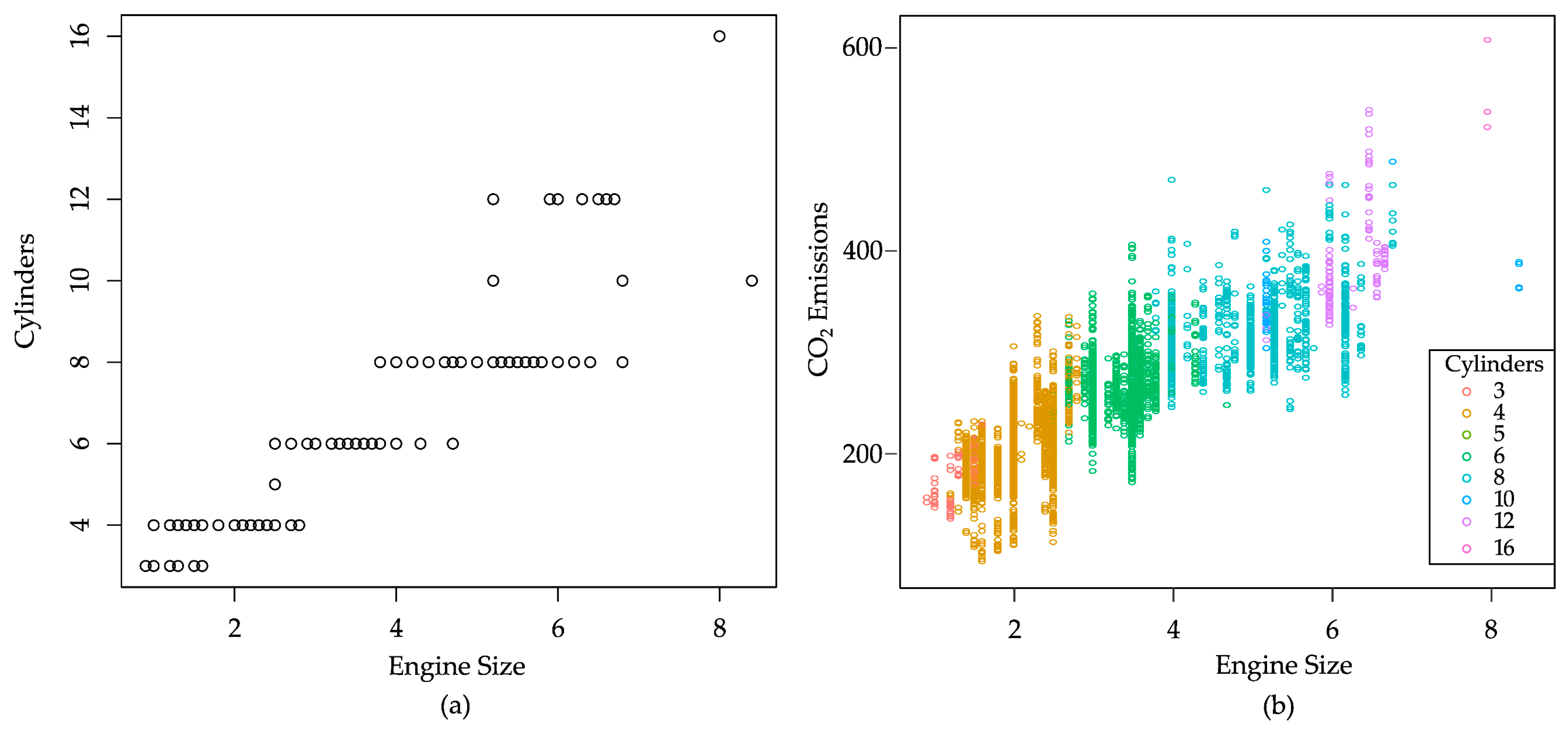
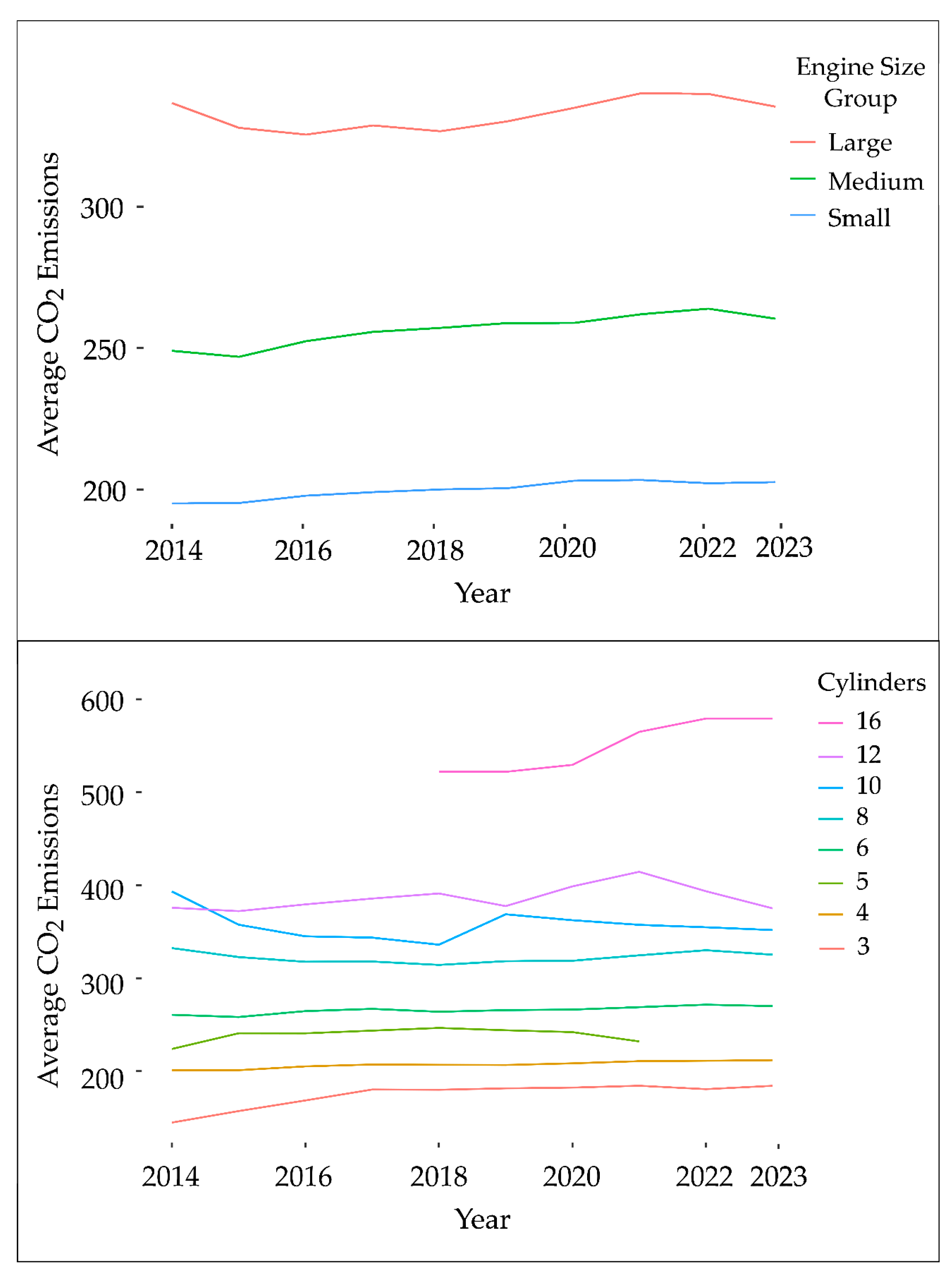
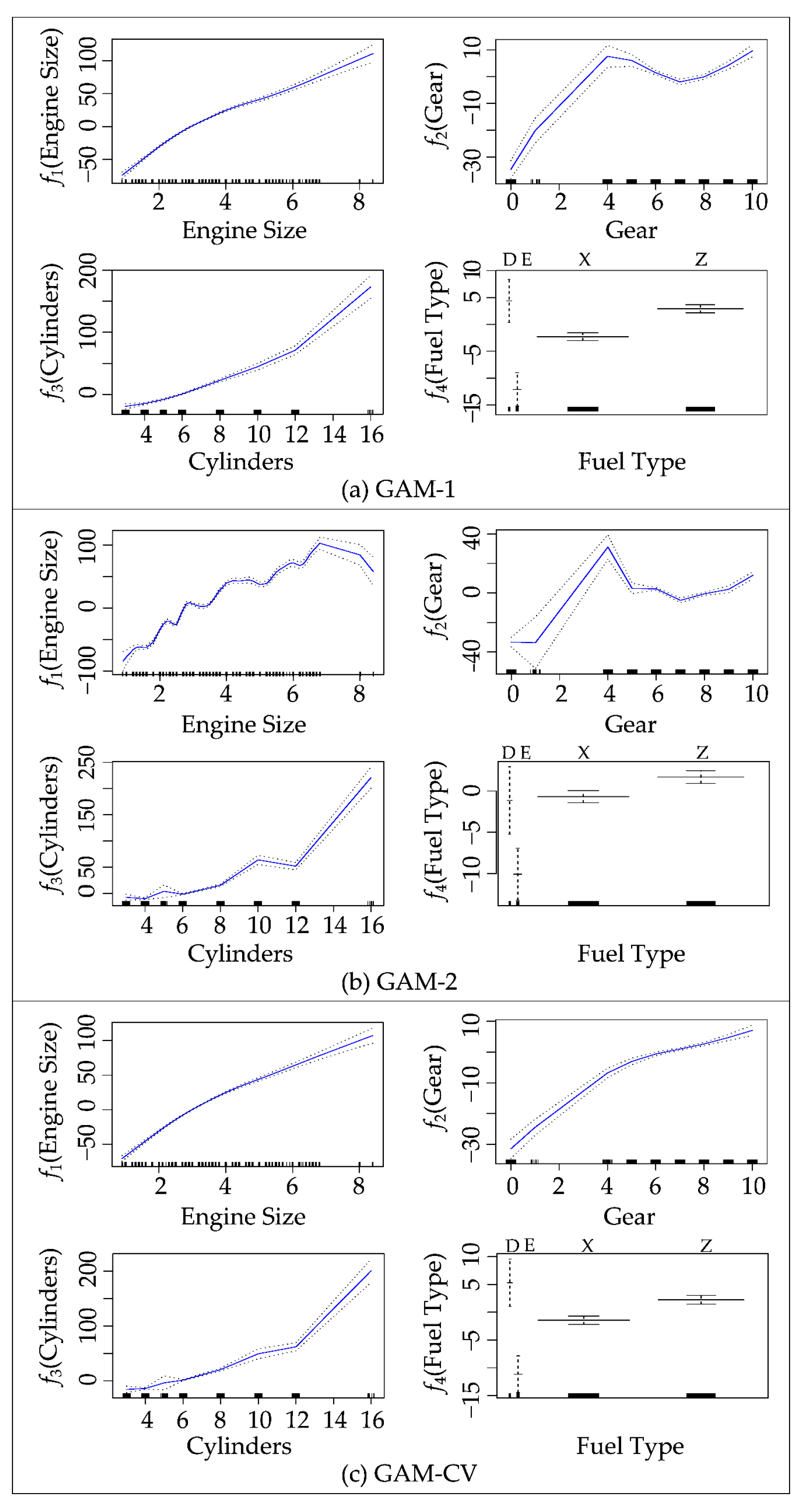
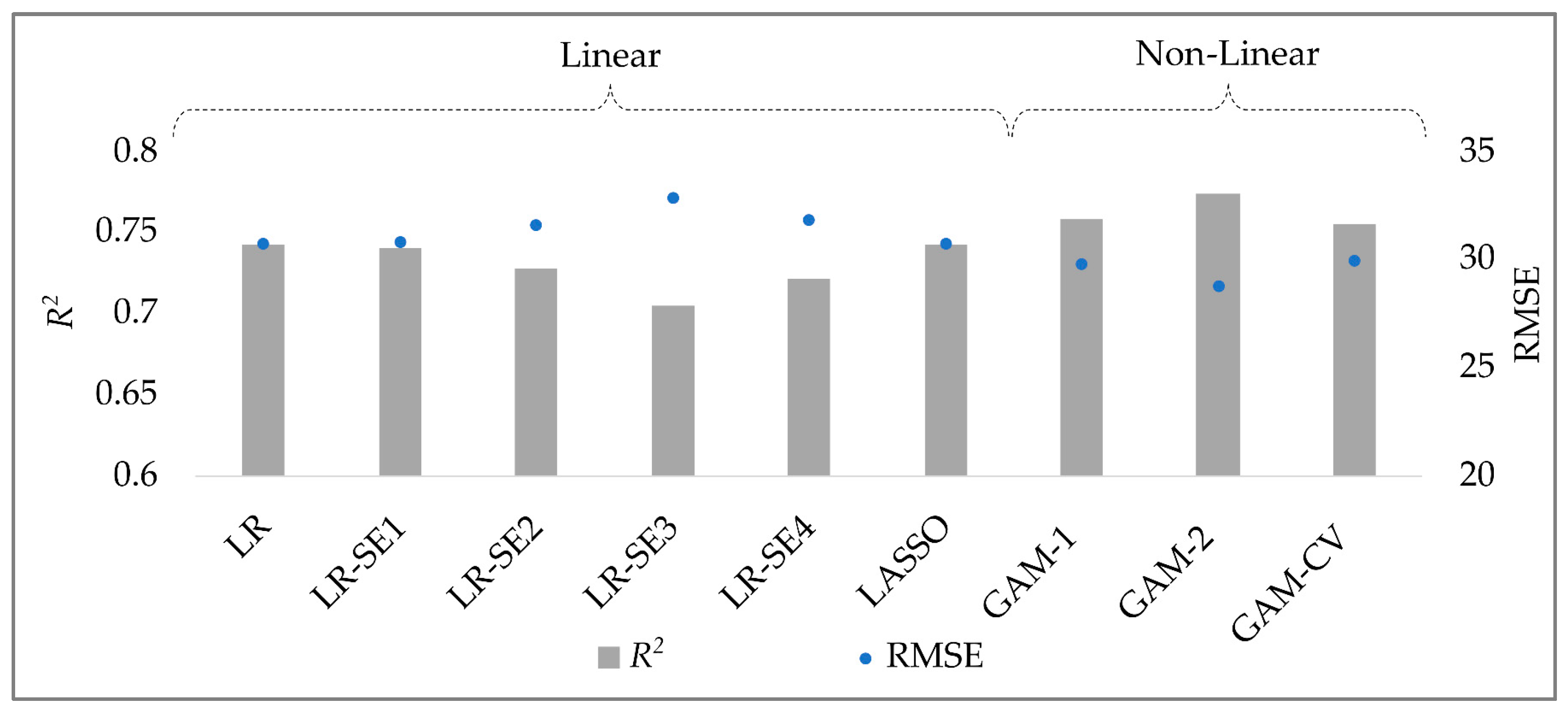
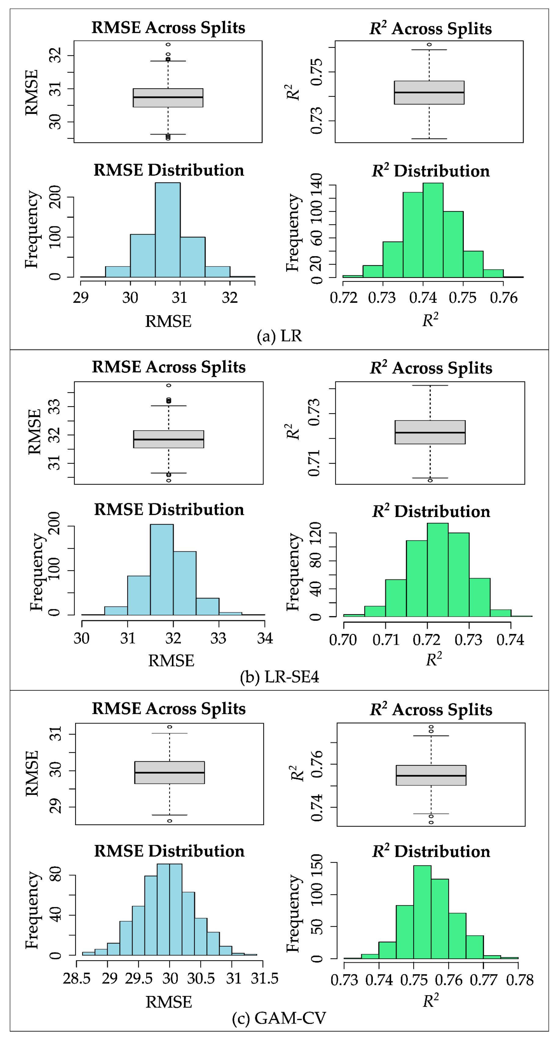
Disclaimer/Publisher’s Note: The statements, opinions and data contained in all publications are solely those of the individual author(s) and contributor(s) and not of MDPI and/or the editor(s). MDPI and/or the editor(s) disclaim responsibility for any injury to people or property resulting from any ideas, methods, instructions or products referred to in the content. |
© 2024 by the authors. Licensee MDPI, Basel, Switzerland. This article is an open access article distributed under the terms and conditions of the Creative Commons Attribution (CC BY) license (https://creativecommons.org/licenses/by/4.0/).