Using Deep Learning to Detect Anomalies in On-Load Tap Changer Based on Vibro-Acoustic Signal Features

Abstract

An On-Load Tap Changer (OLTC) that regulates transformer voltage is one of the most important and strategic components of a transformer. Detecting faults in this component at early stages is, therefore, crucial to prevent transformer outages. In recent years, Hydro Quebec initiated a project to monitor the OLTC’s condition in power transformers using vibro-acoustic signals. A data acquisition system has been installed on real OLTCs, which has been continuously measuring their generated vibration signal envelopes over the past few years. In this work, the multivariate deep autoencoder, a reconstruction-based method for unsupervised anomaly detection, is employed to analyze the vibration signal envelopes generated by the OLTC and detect abnormal behaviors. The model is trained using a dataset obtained from the normal operating conditions of the transformer to learn patterns. Subsequently, kernel density estimation (KDE), a nonparametric method, is used to fit the reconstruction errors (regarding normal data) obtained from the trained model and to calculate the anomaly scores, along with the static threshold. Finally, anomalies are detected using a deep autoencoder, KDE, and a dynamic threshold. It should be noted that the input variables responsible for anomalies are also identified based on the value of the reconstruction error and standard deviation. The proposed method is applied to six different real datasets to detect anomalies using two distinct approaches: individually on each dataset and by comparing all six datasets. The results indicate that the proposed method can detect anomalies at an early stage. Also, three alarms, including ignorable anomalies, long-term changes, and significant alterations, were introduced to quantify the OLTC’s condition.

1. Introduction

Power transformers perform an important role in balancing the voltage levels in the power system. It is therefore very important to check their reliability to prevent the power system from being interrupted [1,2]. Among the power transformer components, the On-Load Tap Changer (OLTC), which is used to regulate the transformer’s output voltage, is identified as one of the most vulnerable parts. Its failure is among the main cause of major power transformers’ catastrophic failures [3,4,5,6]. In this regard, it is necessary to detect OLTC faults in their incipient stages. There are several methods that allow for the detection of OLTC faults. These methods are classified into three categories: (1) offline, (2) on-line, and (3) real-time classes. The offline measurements are performed when the device is de-energized or is out of service. Even though these methods have high accuracy, they need manpower and may be costly due to the required shutdown of the equipment. The online measurements are performed on an energized or in-service device. These methods allow for users to interact with data stored in databases. These data are later accessible from anywhere at any time. The measurements are obtained whenever required. In real-time methods, the measurements also must be continuously acquired from an energized or in-service device [7,8,9]. In addition, real-time systems must respond to events quickly and accurately.

In this work, the vibro-acoustic signals analysis approach, which is an online and real-time method, is used to monitor the OLTC [10]. This technique can detect OLTC faults based on vibro-acoustic signals. These vibroacoustic signals are generated when the OLTC’s moving parts move. Importantly, each OLTC tap position generates a vibro-acoustic signal that can assume similar characteristics to a fingerprint. This means that two vibro-acoustic signals are similar when measured from the same tap position at two different times. Consequently, comparing the latest OLTC vibro-acoustic signals with previous vibration signals helps to detect OLTC faults.

A thorough literature review indicates the development of several approaches to detect an OLTC’s faults based on vibro-acoustic signals. In several works, the OLTC condition is assessed based on the bursts existing in vibration signals. In this regard, features including the number of bursts, the time lag between them, and their amplitude are extracted to analyze the OLTC’s behavior [11,12,13,14]. Specifically Ref. [14] extracted the burst based on the Continuous Wavelet Transform (CWT) technique. The CWT’s vertical ridge plot serves as a straightforward, clear, and visually intuitive method for illustrating fuzzy time domain vibration signals. In addition, the physical sources of the bursts were identified via controlled experiments. In [15,16], the status of each OLTC tap position is analyzed to compare its waveform with a reference; Spearman’s Rank Correlation Coefficient was applied to select the reference waveform. In [17], the condition of the tap changer is evaluated in three steps. In the first step, each vibro-acoustic signal is divided into two parts: preparation, which involves the motor running and driving the mechanical structure, and in-position, which encompasses the operation of the tap-changer. After that, the wavelet packet transform is used to decompose each part into 16 sub-components. Finally, the tap changer is evaluated based on a computation of the energy entropy of each sub-component. In [18], effective band multi-resolution feature parameters are achieved using the wavelet packet coefficients. Then, the Genetic optimization Support Vector Machines (GA-SVM) method is used to classify the mechanical vibration information and identify the mechanical state of the OLTC. Therefore, this methodology succeeds in detecting OLTC faults, and can serve as a reference for the operation and maintenance of OLTCs.

In an effort to develop a real-time monitoring of power transformers’ OLTC, a vibro-acoustic monitoring module was developed and installed on nine single-phase auto transformers in service on Hydro-Québec’s electric network [19]. This system continuously measures vibration signals from the OLTCs and records the signal envelopes. Since the operating temperature affects the vibration signals, this module also measures them. This research aims to develop a global and automatic methodology allowing for a comparison of OLTCs’ vibro-acoustic signals to detect anomalies or malfunctions.

In some previous contributions from the authors [20,21], the temperature effects on vibration signals were addressed. The techniques of averaging and time realignment were applied to discriminate the natural variations in the acoustic signatures of a tap-changer in good condition. It was also shown that changes in vibration signals caused by OLTC faults can be subdivided into two parts, including long-term changes and sudden variation [22]. In the long-term changes, the measured signals related to many previous operations (for example, 600 previous operations) were used for the comparison. In the sudden variation, the measured signals related to a few previous operations (for example, 50 previous operations) were used for the comparison.

In this contribution, the features were extracted from vibration signal envelopes and analyzed afterwards to evaluate the OLTC’s condition. Since the vibration signal envelopes were recorded over several years, each extracted feature from the envelopes (with respect time) falls in the category of time series data. Therefore, methods based on anomaly detection in the time series domain were applied to detect anomalies in the features extracted from vibration signal envelopes.

Recall that, in time series analysis, there are approaches to detect data which do not follow the expected pattern [23]. Two common technical methods that are used to detect anomalies are based on prediction error and reconstruction error [24,25]. In the prediction-error-based algorithms, a model is trained using normal data. After that, the trained model predicts the next instances. The anomalies are extracted based on the prediction error [26]. In the reconstruction-error-based algorithms, normal data are used to train the model. After that, the reconstruction error level of the normal data is determined. Afterwards, anomalies can be detected based on reconstruction error [24]. An autoencoder, a type of neural network, is one of the algorithm-based reconstruction errors used to map the input data. This method tries to reach an output that is very close to the input. Therefore, the output dimension is similar to the input one [24]. Different types of deep autoencoder, such as the LSTM autoencoder, convolutional autoencoder, variational autoencoder, and LSTM variational autoencoder, can be found in the literature [27]. Compared to statistical models, an important reason for the use of the deep learning method in this contribution is the effectiveness and simplicity of deep-learning-based methods. Statistical methods lose effectiveness as the dimensionality of the data increases due to the increase in computational complexity.

In this contribution, a two-step methodology approach is used to detect anomalies in three sister transformer units: (1) online and offline, and (2) three parts including preprocessing, anomaly detection, and the identification of variables responsible for anomalies. In the offline part, the normal dataset is used to build an anomaly detection model and a static threshold is set while, in the online part, recent measurements are analyzed, and the anomalies are detected. The preprocessing part, which is used in both the online and offline parts, is applied to the input dataset to reduce data complexity. Additionally, in this part, the dataset is prepared to undergo both long-term changes and sudden variation. In the anomaly detection part, a model based on an autoencoder (AE) and kernel density estimation (KDE) are used to detect anomalies in continuously measured vibration signal envelopes. In this regard, in the offline section, the AE is trained with a normal dataset and then the reconstruction error is calculated. Later, KDE is fitted to reconstruction errors to compute anomaly scores and a static threshold. In the online section, the recent measurements are evaluated for normality or abnormality. The identification of variables responsible for anomalies is used exclusively in the online section to determine the inputs that are the origin of the anomalies.

It should be noted that a few works have evaluated an OLTC’s condition based on machine learning techniques and vibration signals [28,29]. To the best of the author’s knowledge, deep learning, which has been used to achieve state-of-the-art performance in a wide range of problems, mimicking the learning process of the human brain, is being used for the first time in OLTC monitoring based on vibro-acoustic signal analyses. Even though deep learning is computationally expensive, and requires a large amount of data and computational resources to train, it is best-suited for use in this this study due to its ability to handle large and complex data.

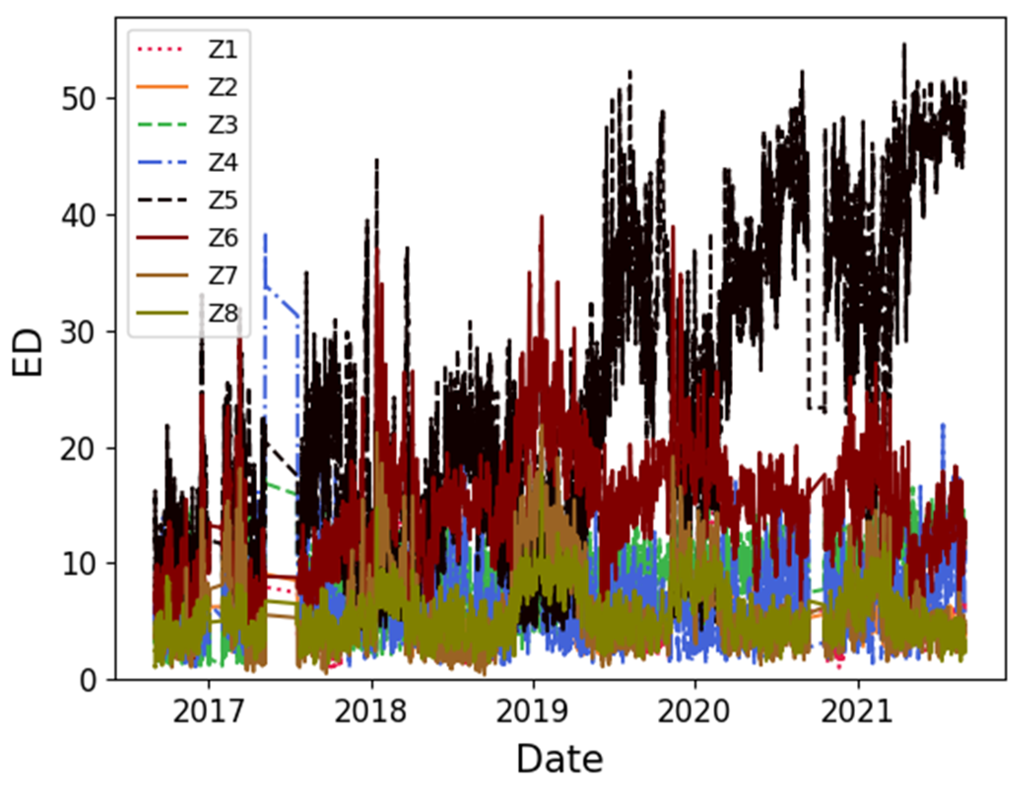
2. Data Collection, Pre-Processing, and Feature Extraction

An OLTC monitoring system designed at the Hydro Québec’s research institute (IREQ) has been installed on nine single-phase autotransformers (rated at 370 MVA, 735/√3/230/√3 kV) in service on Hydro-Québec’s electric network. Vibration signal envelopes are continuously measured and recorded via an accelerometer installed near the diverter switch. Additionally, in this monitoring system, the motor current and temperature are measured and recorded using current clamp and temperature sensors. A detailed description of this monitoring system can be found in [19].

It should be noted that the measured vibration signals are complex and contain a lot of redundant information. In this regard, the Hilbert transformer and Low Pass Filter are applied to extract the signal envelope. After that, the first-order time-realignment technique and moving average are used to discriminate the effect of temperature and to reduce the natural variations in the acoustic signatures of a tap-changer, respectively. These preprocessing techniques were reported by the authors in [20,21].

The research approach is as follows. Three OLTCs associated with three sister transformer units, which are of the ABB UC brand and model, referred to as T3A, T3B, and T3C throughout this paper, are considered as case study units. Vibro-acoustic signal envelopes, with a focus on the segments of the signals, which represent the switching of the OLTC contacts (transformer taps), are derived from the three corresponding OLTCs. By classifying the switching contacts or transformer taps as odd and even, the datasets are divided accordingly, resulting in six subsets: T3A-odd, T3A-even, T3B-odd, T3B-even, T3C-odd, and T3C-even (illustrated in Figure 1) [19]. In Figure 1, the moving average of 10 consecutively measured vibration signal envelopes is depicted in grey, while the reference data for each dataset are represented in black. The utilization of a realignment algorithm to compensate for the temperature effects on these datasets is notable.

To monitor the OLTC’s condition, useful features should be extracted from the measured vibration signal envelopes. In this regard, the main zones are extracted automatically (see blue zones in Figure 1) based on the location of the main peaks. To detect the main peak location, at first, the location of the main peak in the reference is detected. After that, the main peaks in each vibration signal envelope are detected based on the reference main peak’s location. Later, Euclidean distance (ED) is computed between each zone in each envelope, realigned with time. The ED of the main zones in the T3A-odd dataset is shown in Figure 2. The details of the extraction of main zones are explained in the author’s recent contribution [19].

3. The Underlying Concept

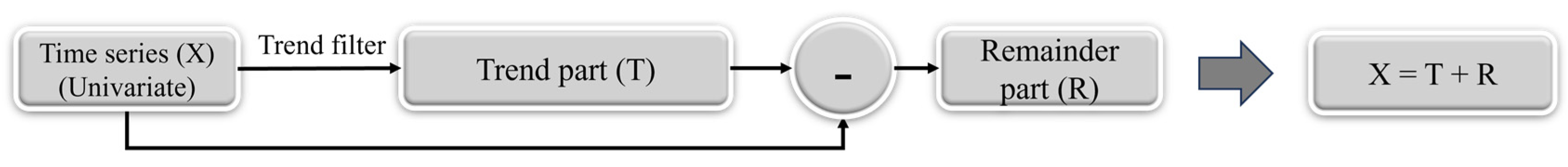
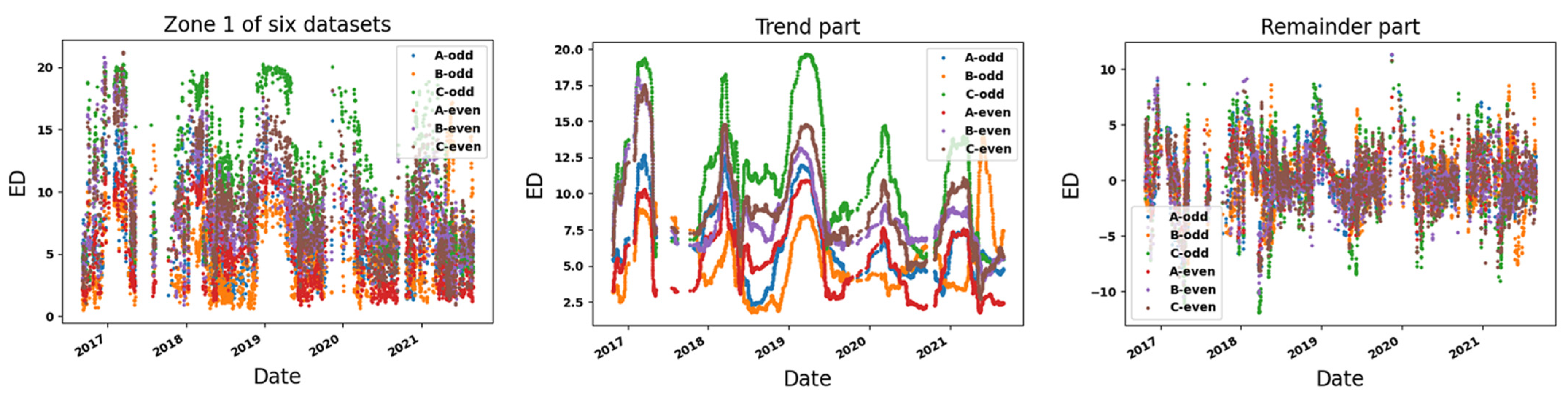
3.1. Time Series Decomposition

A time series can be split into different components. Generally, there are two types of decomposition, including additive and multiplicative. Based on these categories, a time series can be decomposed into three components: Trend (the overall trend in the time series), Seasonal (repeating patterns), and Residual (primarily considered to be noise). The decomposition function, based on addition and multiplication, is shown in Equations (1) and (2), respectively [30]. It is important to note that there is a delay in the real-time trend decomposition process, as this involves the utilization of past data at each time step (using non-symmetric filters) to calculate the trend [31].

$$X\left(t\right)=\mathrm{T}\mathrm{r}\mathrm{e}\mathrm{n}\mathrm{d}\left(t\right)+\mathrm{S}\mathrm{e}\mathrm{a}\mathrm{s}\mathrm{o}\mathrm{n}\mathrm{a}\mathrm{l}\left(t\right)+\mathrm{R}\mathrm{e}\mathrm{s}\mathrm{i}\mathrm{d}\mathrm{u}\mathrm{a}\mathrm{l}\left(t\right)$$

(1)

$$X\left(t\right)=\mathrm{T}\mathrm{r}\mathrm{e}\mathrm{n}\mathrm{d}\left(t\right)\times \mathrm{S}\mathrm{e}\mathrm{a}\mathrm{s}\mathrm{o}\mathrm{n}\mathrm{a}\mathrm{l}\left(t\right)\times \mathrm{R}\mathrm{e}\mathrm{s}\mathrm{i}\mathrm{d}\mathrm{u}\mathrm{a}\mathrm{l}\left(t\right)$$

(2)

3.2. Deep Autoencoder-Based Anomaly Detection

Another time series anomaly detection technique is based on reconstruction error. In this technique (Figure 3), a model is used to copy the input to the output. The model can therefore learn the pattern between the data. In the training step, the model improves itself to minimize the reconstruction error. After the training step, it is expected that the trained model will generate an output that is close to the input (lower reconstruction error) with the normal data and generate an output that is far from the input (higher reconstruction error) with the abnormal data. Consequently, anomalies can be detected using the reconstruction error. A popular technique that is used to reconstruct the input is through the use of autoencoders [27].

Anomaly detection based on an autoencoder is one of the best machine learning methods to detect anomalies in a time series [32]. As shown in Figure 4, an autoencoder consists of an encoder and a decoder [33]. An encoder is used to reduce and compress the input dimension ($X$) to a latent space ($Z$), whereas a decoder is applied to decompress the encoded representation ($Z$) into the output layer ($\widehat{X}$). Therefore, the input and output have the same dimension [34]. In deep learning, autoencoders use several hidden layers to reduce the dimension of the data. In hidden layers, the number of units is reduced hierarchically and, in this process, it is expected that hidden units will select features that well represent the data [35].

In time series anomaly detection, an autoencoder is trained with a normal training dataset. After that, the trained autoencoder predicts the training set. Later, the difference between the input and output is computed and a reconstruction error vector is obtained. This vector can be used to calculate the threshold. In this work, the metric of mean squared error (MSE) is used to compute the reconstruction error.

Various types of autoencoders exist, such as convolutional autoencoders, RNN autoencoders, LSTM autoencoders, and variation autoencoders [24,34,35]. For this study, a convolutional autoencoder was utilized to monitor the OLTC’s condition. The reason for selecting this type of architecture is that it is not fully connected, allowing it to delve deeper and undergo faster training. This type of autoencoder is based on a convolutional neural network. In a convolutional neural network architecture, convolution layers with kernels serve as adaptable filters that slide across the time steps and variables, capturing temporal patterns and relevant features. Pooling layers are generally used for the temporal down-sampling to further extract the information. In an autoencoder, the convolutional layer, and sometimes the pooling layer, are used in the encoder. In the decoder, convolution transpose layers (also known as deconvolutional layers) and up sampling layers are employed to reconstruct the encoded input [24,36].

3.3. One-Class Classification

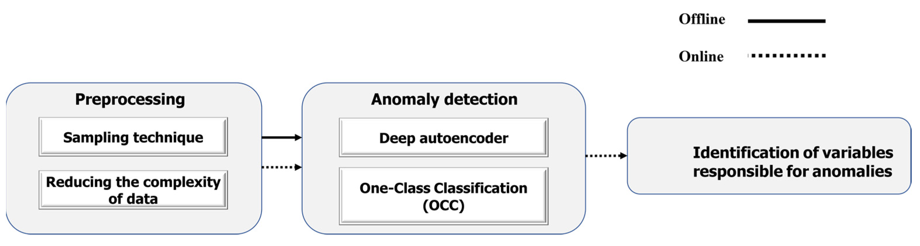
One-class classification (OCC), which is a particular case of multi-class classification, is used in the anomaly detection concept. According to OCC, there is only one class used to construct a classifier [37,38]. Figure 5 shows the concept of OCC. As shown in this figure, there is one class, and the data that are placed inside the class are considered normal. In this type of classification, there are two types of objects, which are referred to as target and outlier objects. The objects inside the class are considered the target objects, while all other ones are assumed to be the outlier objects. Therefore, the data inside the class are considered normal and each new piece of data should be analyzed to detect whether it resembles the class or not [39]. KDE is a nonparametric method and can directly estimate density from the data. This technique can be used as a one-class classifier by applying a density threshold. In this regard, the data that are of low density are considered abnormal.

KDE is used to estimate a probability density function from a sample of points without any assumption about the underlying distribution. There are two factors, including kernel function and bandwidth, which play an important role in KDE. There are different types of kernel functions, such as exponential, Epanechnikov, and Gaussian. The Gaussian kernel is most popular in applications and was also used in this work [38]. Bandwidth is used to determine the smoothness of the resulting density function. Selecting a very small bandwidth value generates a rough density function. However, selecting a very large value smooths out any true features of the underlying distribution [40].

4. Methodology

The proposed methodology is illustrated in Figure 6. As shown in this figure, the methodology consists of three parts, including preprocessing, anomaly detection, and the identification of variables responsible for anomalies. In the following, each part of the methodology is explained in detail.

4.1. Preprocessing

4.1.1. Sampling Method

The sampling technique is applied, with the goal of comparing the six datasets. Instead of comparing the whole datasets, a subset from each dataset is isolated and used. In this regard, the data values that were measured at the same time (year, month, hour, minute) are separated from each dataset.

4.1.2. Reducing the Complexity of Data

The theory of decomposition is used to reduce the complexity of the data. As shown in Figure 7, a trend filter is applied to a time series and the trend in the data is separated. After that, the trend is subtracted from the whole time series to obtain the rest of the data (called the Remainder). As such, each part is individually evaluated to detect anomalies.

Furthermore, a simple moving average is employed to capture the trend component [31]. This technique utilizes a window size to characterize the trend component. It is worth noting that the selection of the window size is crucial. When a small window size, such as 50, is selected, the local trends and sudden variations can be captured. However, when a large window size, such as 500, is selected, the global trends and long-term changes can be captured. Subsequently, each univariate time series is decomposed into two components, the Trend and Remainder, and each component is evaluated individually to identify anomalies. This step is performed twice, using the different window sizes of 50 and 500, in the individual analysis of each dataset, while only window size 50 is used in the comparative analysis. As mentioned, there is a delay in the Trend part because the simple moving average is applied non-symmetrically.

4.2. Anomaly Detection

The procedure used to detect anomalies is presented in Figure 8. As shown in Figure 8, anomaly detection is achieved in two ways: offline and online. In the offline technique, after the preprocessing, an autoencoder model is trained with normal data and the reconstruction errors are computed. After that, the anomaly scores of the normal data and the static threshold are computed based on KDE. In the online technique, the trained model is stored in the detection part. A new observation after preprocessing is entered into the online sector and its reconstruction output is established. After that, the reconstruction error is computed, and then its anomaly score is calculated based on the fitted KDE. Finally, if its anomaly score is lower than a dynamic threshold, the new observation is considered abnormal. In the following, the three steps of anomaly detection, including preprocessing, the offline sector, and the online sector, are explained in detail.

4.2.1. Preprocessing

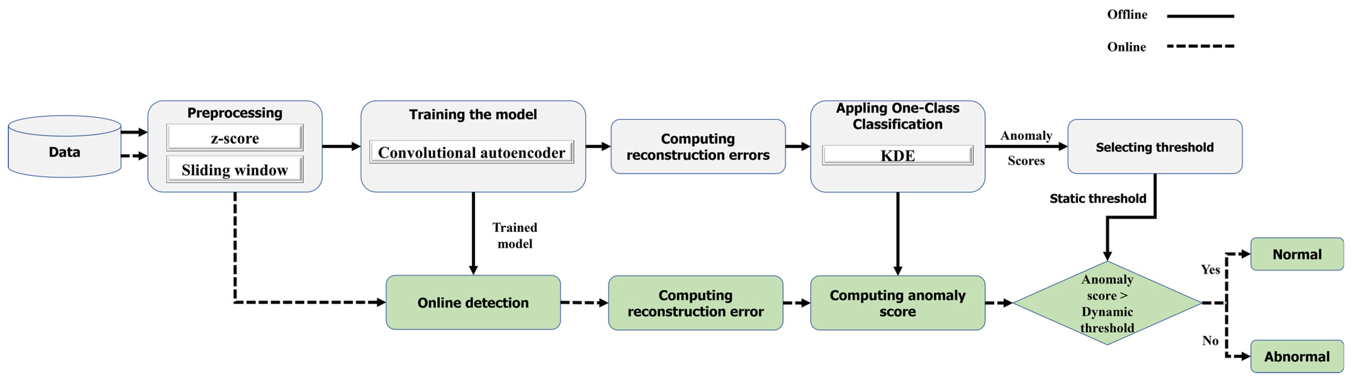
• Standardization: z-score function, presented in Equation (3), is used to standardize the time series data [41].

  $$z=\frac{X-\mu }{\sigma }$$

  (3)

where $\mu$ and $\sigma$ represent the average and standard deviation of the data.

• Sliding window: A time series can be subdivided into several parts of the same size using the sliding window technique. In this technique, there are two indicators, including window size (W) and step size (s), which indicate the length of the window and the amount of stride in subsequent windows, respectively. In this work, a sliding window with s = 1, which causes the creation of overlapping windows, is applied to achieve a short time series (parts).

4.2.2. Offline Sector

The offline sector includes two parts. In the first part, the model is trained with normal data and, later, the reconstruction error of the normal data is computed. In the second part, KDE is trained with the reconstruction errors and, after that, the log-likelihood of the reconstruction errors in the normal data is computed. It should be noted that a static threshold is also defined in this part.

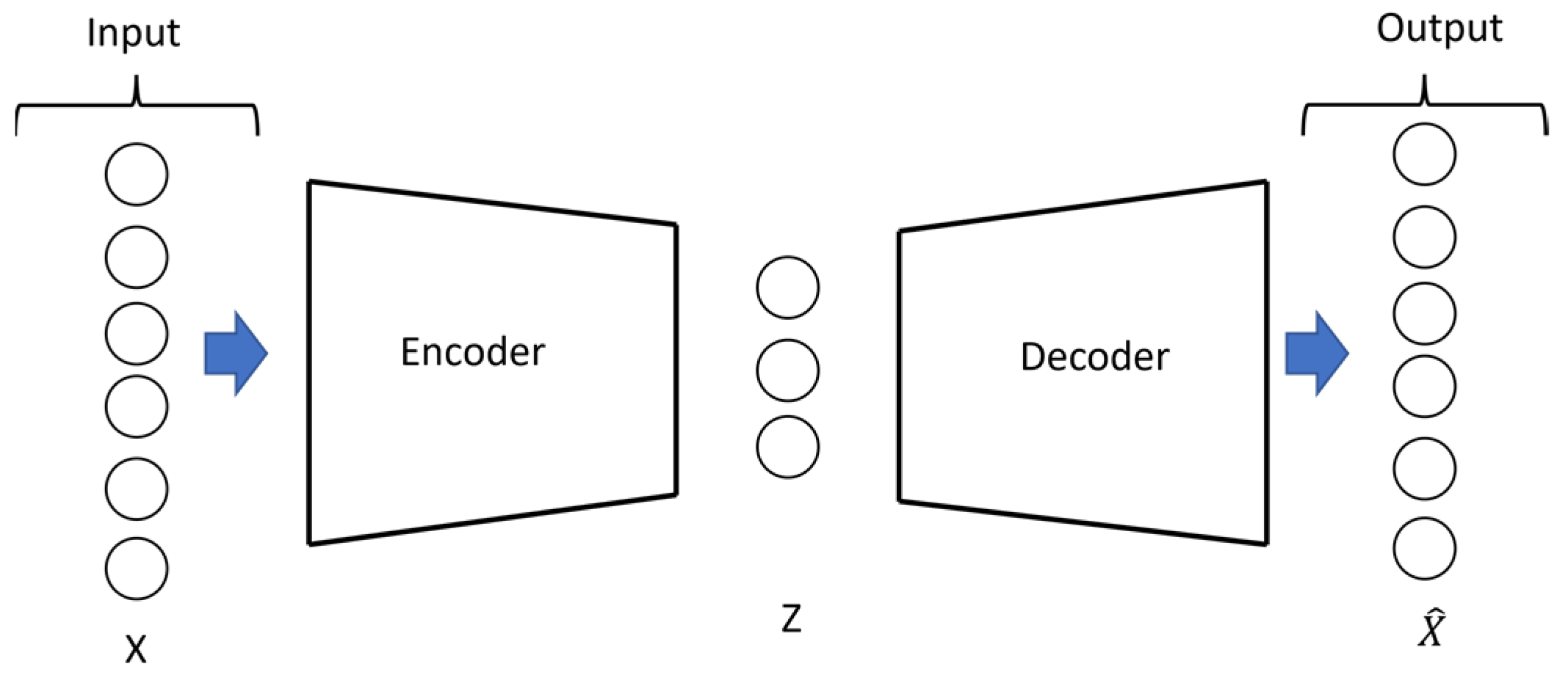
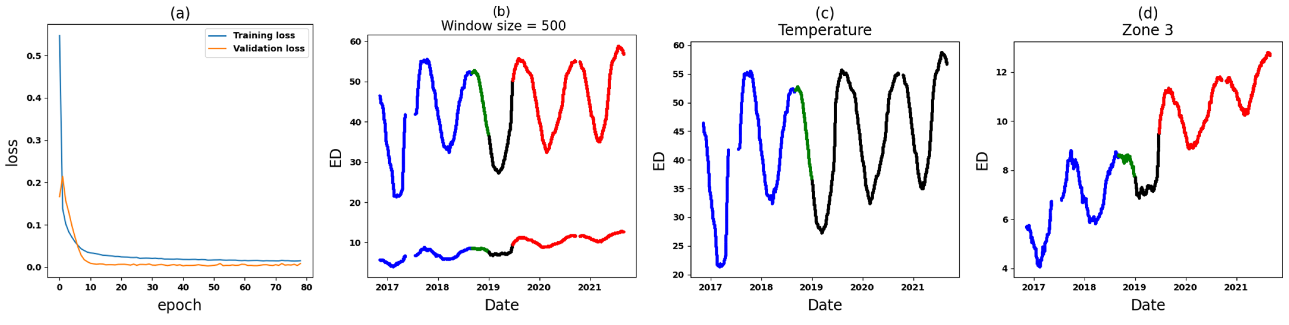
• Training the model: A convolutional autoencoder is used as a model to detect anomalies. In this model, the encoder and decoder use two layers. It is important to note that the model is trained using a set that contains normal data. Additionally, a validation set containing normal data is utilized to prevent overfitting and to determine when to halt the training process.
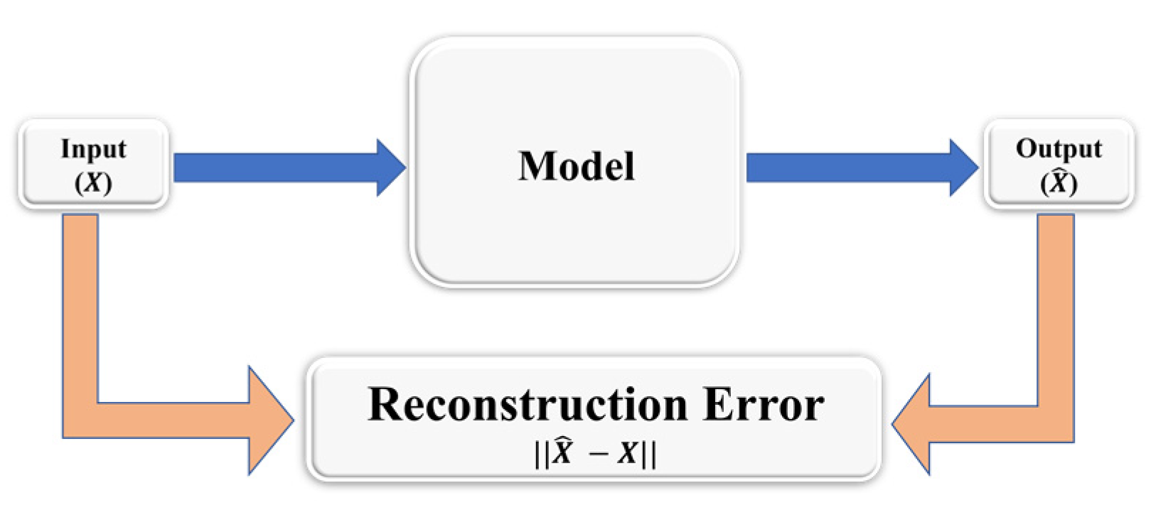
• Reconstruction errors are computed between the original (X) and reconstructed ($\widehat{X}$) data. MSE is then used to compute the reconstruction error.
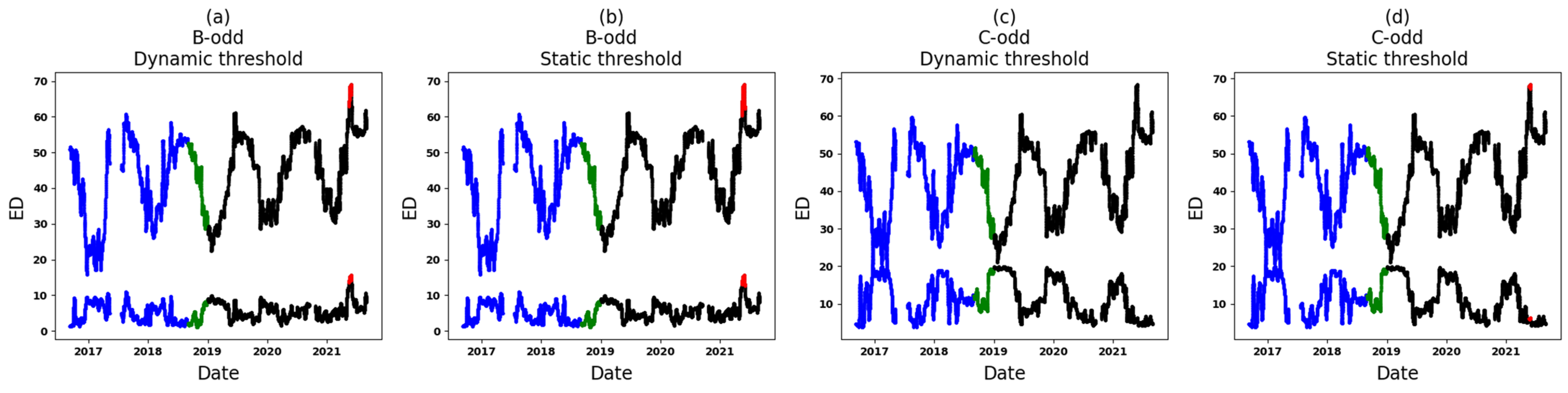
• The Application of One-Class Classification (extracting anomaly scores based on KDE and selecting a static threshold): During this stage, the KDE method is utilized and tailored to the reconstruction errors of the training set. Following this, the log-likelihood of every instance in both the training and validation sets is calculated. This reconstruction log-likelihood is used as the anomaly score in the anomaly detection model. As such, a high score indicates that the input $X$ is suitably reconstructed. The threshold is determined by considering the minimum anomaly score found within both the training and validation sets. It should be noted that the threshold is rounded down to the nearest whole number. This means that values such as 2.1 and 2.7 would be rounded down to 2.

4.2.3. Online Sector

The recent measurement (new observation) obtained after the preprocessing steps is entered into the online sector. In the first step, the reconstruction value of the recent measurement is achieved using the trained model. After that, the reconstruction error is computed and, later, its anomaly score is calculated using fitted KDE. Finally, if the anomaly score of the new observation is less than a dynamic threshold, this observation is labeled abnormal; otherwise, it is marked as normal. It should be noted that the smaller anomaly score means that it does not follow the normal pattern.

The dynamic threshold can be calculated based on k anomaly scores before recent measurements. According to this strategy, k anomaly scores before recent measurements are selected and KDE is fitted with these values. Then, the log-likelihood of each value is computed based on the fitted KDE. Finally, a dynamic threshold is obtained by summing the minimum value between the log-likelihood values (of k anomaly scores before recent measurements) and the static threshold.

4.3. Identification of Variables at the Origin of Anomalies

Because the anomaly detection system relies on multiple variables, when an anomaly occurs, it is essential to identify the variables at the origin. To explain how an anomaly is detected, the reconstruction error calculation process should be clarified.

$\mathrm{M}\mathrm{S}\mathrm{E}$ is used to calculate reconstruction errors. For example, if the input has two dimensions ($X$ and $Y$) and a sliding window as a third dimension, the actual value and its reconstruction value for recent measurements are shown in Equations (4) and (5), respectively. $MSE$ is individually computed for each input variable, and is shown in Equation (6). After that, the standard deviation of the $MSE$ vector is computed and the variable that has a higher $MSE$ value than the standard deviation is considered as the root of the anomaly. With this strategy, it is possible to have more than one variable as the root of anomalies.

$$\left[\left[X_t{Y}_t\right]\left[X_{t-1}{Y}_{t-1}\right]\left[X_{t-2}{Y}_{t-2}\right]\right]$$

(4)

$$\left[\left[{\widehat{X}}_t{\widehat{Y}}_t\right]\left[{\widehat{X}}_{t-1}{\widehat{Y}}_{t-1}\right]\left[{\widehat{X}}_{t-2}{\widehat{Y}}_{t-2}\right]\right]$$

(5)

$$\left[{MSE}_X{MSE}_Y\right]$$

(6)

5. Results

The proposed algorithms were implemented in Python 3.9.5, and PyCharm 2021.2.3, which provides an Integrated Development Environment (IDE) for Python. The Keras library was utilized, employing layers of Conv1D. Conv1DTranspose and Dropout operations were used to create a convolutional autoencoder. The convolutional autoencoder architecture comprises both encoding and decoding components. The encoder consists of two consecutive Conv1D layers with n (the number of filters) and n/2 filters, respectively. These layers are used to reduce the dimensionality and extract essential features from the input data. The decoder starts with a Conv1DTranspose layer with n/2 filters, followed by another Conv1DTranspose layer with n filters. These decoder layers are responsible for reconstructing the input data from the latent space representation. The dropout layers with a rate of 0.2 are inserted after the first encoding and decoding layers to prevent overfitting. In addition, loss functions and mean squared error (MSE) are used. It is important to note that another Conv1DTranspose layer (the final layer) is used to return the output to the original input dimensionality. In addition, several hyperparameters are optimized, including activation, the number of filters (n), the optimizer, and the batch size. For the activation parameter, two options, tanh and relu, are considered. The n parameter can be either 16 or 32. In terms of optimizers, two options are tested: Adam, with a learning rate of 0.001, and Adamax, with the same learning rate. Finally, the batch size parameter is explored with values of 128 and 256.

The six datasets were analyzed using two distinct strategies: one involves a comparative analysis of six databases, while the other entails an individual analysis of each dataset. Additionally, each dataset is individually analyzed based on two steps: long-term changes and sudden variations. Consequently, Zones 1, 3, and 5 from the six datasets were extracted and compared individually. The data for these zones are presented in Figure 9 from left to right, respectively. Furthermore, each of these zones was analyzed individually in each dataset, and it should be noted that temperature was also included as an input in the individual analysis of each dataset. To avoid repetition, the results of T3A-odd and T3B-odd were discussed separately during individual analyses. Zones 1, 3, and 5, with temperature in T3A-odd and T3B-odd, are shown in Figure 10 and Figure 11.

The OLTC anomalies are detected using two strategies: an individual analysis of each dataset and a comparative analysis. Furthermore, in the preprocessing stage, to achieve the Trend and Remainder parts, window sizes of 50 and 500 are employed in the individual analysis of each dataset, while a window size of 50 is considered in the comparative analysis. Figure 12 illustrates an example of the decomposition step for Zone 1 of the six datasets (comparative analysis). After that, each of these parts (the trend and remainder) is subdivided into two groups. The first group contains normal data. This group of data is subdivided into training and validation sets. The second group includes normal and sometimes abnormal data, and this group is called the test set. The convolutional autoencoder is trained using the training set (normal data). The validation set is used to avoid model overfitting. Finally, the test set is used to evaluate the model. In the following, the results related to OLTC anomalies are shown. It should be noted that, within the entire dataset, the data from 1 September 2016, to 1 September 2018, (two years) are considered the training set. The data spanning from 1 September 2018, until 1 January 2019, (four months) are also considered part of the validation set. The remaining data, from 1 January 2019, to 1 September 2021, are referred to as the test set.

5.1. Comparative Analysis

The results of anomalies in Zones 1, 3, and 5, illustrated in Figure 9, are compared in Figure 13, Figure 14 and Figure 15, respectively. Consequently, subfigure (a) presents the training loss and validation loss of the model versus the number of epochs. In the other subfigures, the training, validation, and test sets are represented by blue, green, and black colors, respectively. Additionally, the detected anomalies in the test set are displayed in red. It should be noted that subgraph (b) shows all input variables and the detected anomalies using a dynamic threshold, while subgraphs (c), (d), (e), (f), (g), and (h) display the root of the anomalies shown in subgraph (b) in red. As indicated in these subgraphs, it is possible that the root of anomalies includes more than one input variable.

5.2. Individual Analysis of Each Dataset

As previously mentioned, the individual analysis of each dataset involves two distinct steps: identifying anomalies related to long-term changes and identifying anomalies related to sudden variations. Consequently, window sizes of 500 are used during the preprocessing step (decomposition) to capture long-term changes, while window sizes of 50 are employed to detect sudden variations. In this section, an examination of Zones 1, 3, and 5 is conducted within both the T3A-odd and T3B-odd datasets to identify anomalies associated with either long-term changes or sudden variations. Anomalies linked to sudden variations are notably detected in Zones 1 and 3 of dataset T3B-odd, showcased in Figure 16 and Figure 17, and in Zones 3 and 5 of dataset T3A-odd, showcased in Figure 18 and Figure 19, respectively. Moreover, anomalies attributed to long-term changes are identified in Zones 3 and 5 of dataset T3A-odd, presented in Figure 20 and Figure 21, along with Zone 3 of dataset T3B-odd, presented in Figure 22, respectively.

In these figures, subgraph (a) displays the model’s training and validation losses concerning the number of epochs. Subgraphs (b), (c), and (d) represent the training, validation, and test sets in blue, green, and black colors, respectively. Furthermore, anomalies detected in the test set are highlighted in red. Subgraph (b) exhibits all input variables along with the detected anomalies using a dynamic threshold, while subgraphs (c) and (d) display the variable responsible for the anomalies depicted in subgraph (b) using the color red.

It should be noted that the remaining parts were also analyzed, and a few anomalies were detected in the comparative analysis, while no anomalies were found in the individual analyses. Therefore, no significant anomalies were detected in the remaining parts.

6. Discussion

In this contribution, a convolutional autoencoder and KDE are used to detect anomalies in the extracted features from vibro-acoustic signal envelopes. In addition, in a preprocessing step, the sampling method and trend filter are used to reduce the complexity of the input data. Moreover, standard deviation is utilized to identify the variables that are the origin of anomalies. To evaluate the proposed methodology, Zones 1, 3, and 5 were selected. Recall that Zones 1, 3, and 5 are not random selections. In fact, they were chosen deliberately to assess the proposed methodology. Notably, Zone 3 consistently exhibits a smooth, consistent change, indicative of long-term changes across all datasets. Furthermore, a distinctive pattern is observed in Zone 5 of T3A-odd compared to Zone 5 in other datasets [19]. Based on the findings of anomalies in Section 5, the following observations are made for each Zone, individually.

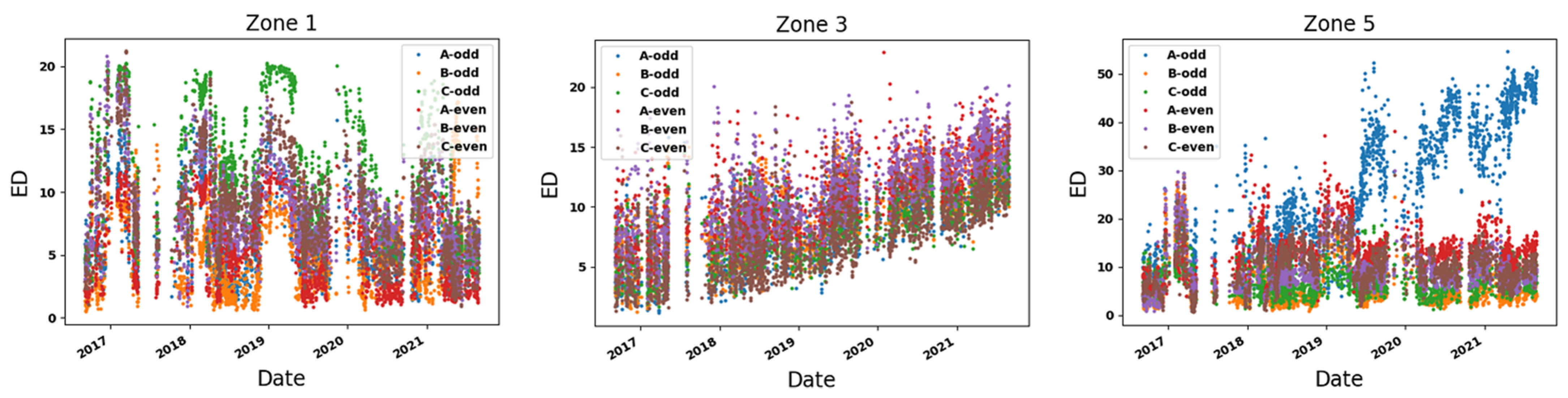
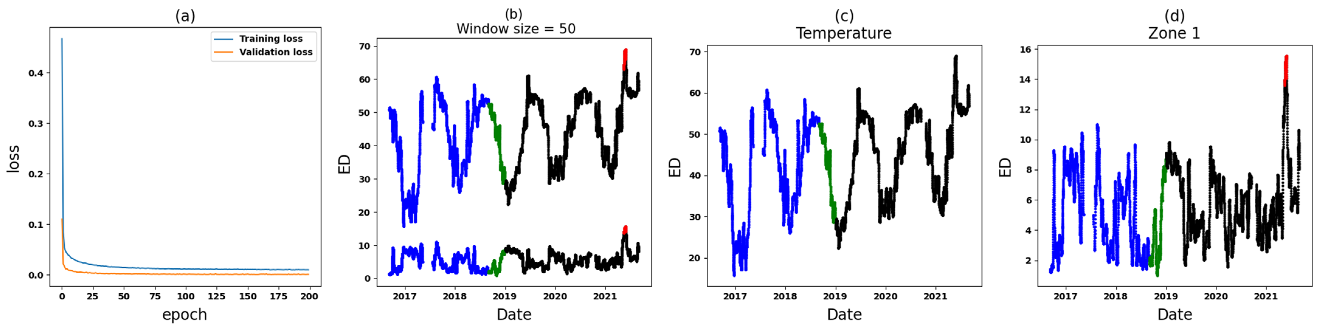
• Zone 1: In the comparative analysis, anomalies are identified in a specific segment of the test set (see Figure 13). Following this, Zone 1 of T3A-odd and Zone 1 of T3B-odd are individually scrutinized. Based on the outcomes of the individual analyses, anomalies attributed to sudden variations are found specifically in T3B-odd (see Figure 16). These anomalies continue for around 14 days, after which there are no further anomalies. Consequently, it can be inferred that there might not be a significant cause for concern or an important alarm.
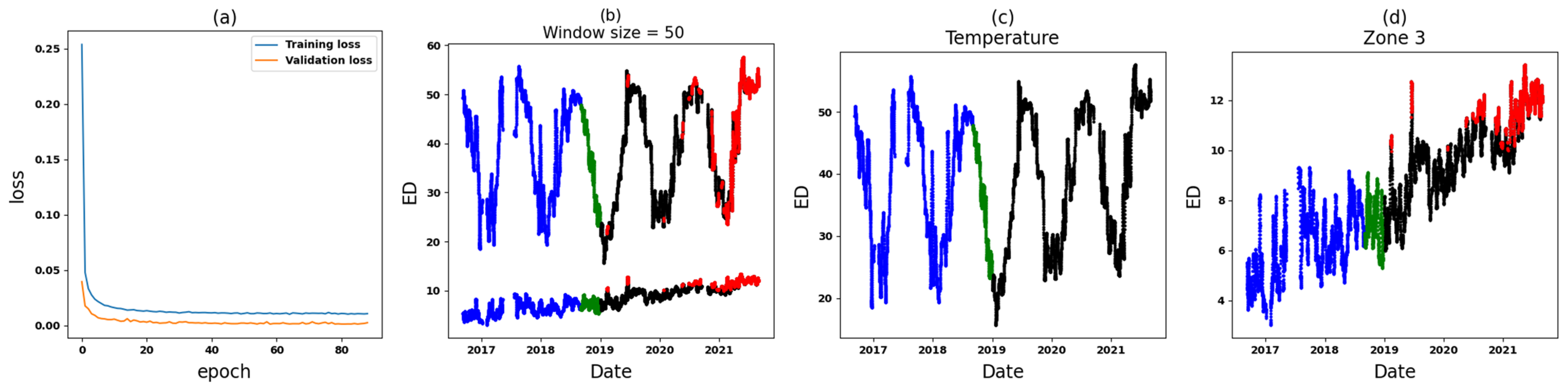
• Zone 3: In the comparative analysis, anomalies are observed spanning from 9 June 2019, until the end of September 2021 (see Figure 14). Notably, a crucial observation within this timeframe is that all input variables (Zone 3 in six datasets) are implicated as the cause of these anomalies, causing significant concern. To further understand the circumstances within this zone, Figure 17 and Figure 18 depict the results for Zone 3 of the T3B-odd and T3A-odd datasets, respectively, based on sudden variation. Additionally, Figure 20 and Figure 22 illustrate the results for Zone 3 of the T3A-odd and T3B-odd datasets, respectively, based on long-term changes. Upon examination of these figures, while some anomalies are identified based on sudden variations, it is evident that long-term changes are prevalent in this area. Consequently, the presence of persistent long-term changes raises an important alarm within this particular zone.
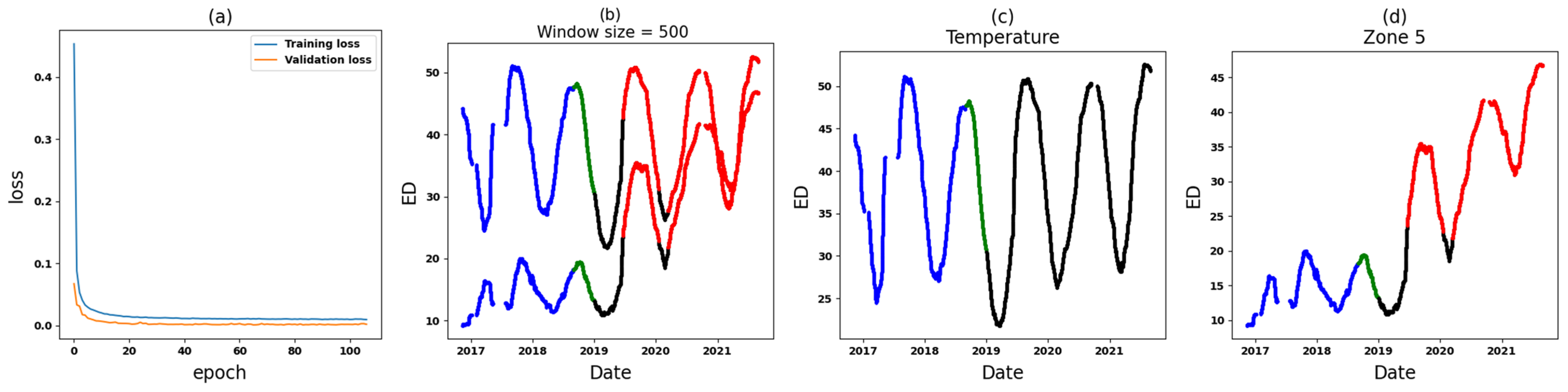
• Zone 5: In the comparative analysis, anomalies were consistently observed since 9 June 2019. Primarily, these anomalies are attributed to T3A-odd (refer to Figure 15). Upon conducting individual analyses of Zone 5 within both T3A-odd and T3B-odd datasets, continuous anomalies are detected solely in Zone 5 of dataset T3A-odd, indicating occurrences associated with both sudden variations and long-term changes. Notably, no anomalies were found in Zone 5 of the T3B-odd dataset. Consequently, these findings strongly suggest that significant alterations occurred specifically within Zone 5 of the T3A-odd dataset (see Figure 19 and Figure 21).

Based on the above-mentioned points, anomalies can be categorized into three types of alarms: ignorable anomalies, long-term changes, and significant alterations. An analysis of anomalies in Zone 1 reveals the presence of anomalies that can be disregarded. These anomalies likely stem from natural variations such as temperature fluctuations because they occur within a short period; no further anomalies are observed afterward. In Zone 3, the anomalies suggest the existence of long-term changes. Although these changes might not immediately cause faults, they have the potential to create faults in the future. Meanwhile, Zone 5 indicates significant alterations within Zone 5 of T3A-odd, implying the potential occurrence of faults in the near future.

It would be beneficial to note that our application of deep learning for anomaly detection initially encountered challenges due to the complexity of the input variables. However, through rigorous preprocessing steps, including the sampling method and the application of a trend filter, significant improvements were achieved. These preprocessing techniques proved invaluable in managing the complexity of the input data and enhancing the performance of the deep learning model.

Furthermore, the performance of the proposed method was evaluated based on two strategies: an individual analysis of each dataset and a comparative analysis. Although the number of input variables differs between the two strategies, the proposed method is able to detect anomalies as well as identify the variables at the origin of these anomalies. Therefore, the methodology is globally applicable and can be used for any OLTC that has the same monitoring system as that mentioned in this paper.

It should be noted that this work utilizes a dynamic threshold instead of a static one. To compare the anomaly results obtained from dynamic and static thresholds, Zone 1 of T3B-odd and T3C-odd were selected. It is worth mentioning that a window size of 50 was used to establish the trend part. The anomalies based on the dynamic and static thresholds for Zone 1 (trend part) of T3B-odd and T3C-odd are depicted in Figure 23, Subgraphs (a), (b), (c), and (d), respectively, in red. As illustrated in these figures, the dynamic threshold was used to disregard anomalies that do not represent a significant cause for concern. Consequently, there are no anomalies in Zone 1 of T3C-odd based on the dynamic threshold (see Subfigure (c)), whereas anomalies exist based on the static threshold in this zone (see Subfigure (d)). Furthermore, it is worth noting that there are more anomalies in Zone 1 of T3B-odd based on the static threshold than the dynamic threshold (see Subfigures (a) and (b)). In future works, the impact of temperature on the vibration signal envelope will be investigated. The aim is to discriminate the effect of temperature (natural variation) on vibration signals.

7. Conclusions

In this research work, the vibro-acoustic signal analysis technique was employed to monitor the power transformer OLTC’s health condition. In this context, the vibration signal envelopes generated by the OLTC of three transformers over the past few years were measured. It is important to note that these envelopes were aligned, and the main zones were extracted from them. Subsequently, the ED metric was used to compute the similarity between the monitored envelopes and the reference; this metric was computed on the corresponding zone. In this regard, the extracted feature (ED computation) from the envelopes (with respect to time) was considered in the category of time series data. Based on these features, a new methodology comprising three parts, i.e., preprocessing, anomaly detection, and the identification of variables responsible for anomalies, was developed to detect the behavior of a power transformer OLTC. According to this methodology, each univariate feature was divided into two sectors, the trend and remainder sections, based on a moving average strategy. The decomposition facilitates the capturing of long-term changes and sudden variations. Subsequently, anomalies were detected in each sector based on a multivariate convolutional autoencoder and KDE. Initially, a convolutional autoencoder was applied to obtain reconstruction errors, and KDE was utilized to fit the reconstruction errors to compute the anomaly score, static threshold, and dynamic threshold. Then, a statistical parameter, standard deviation, was used to identify the variables responsible for the anomalies. This proposed methodology was evaluated using six different real datasets via two strategies: comparing OLTC sisters and performing an individual analysis for each dataset. The obtained anomaly results allow for the creation of three distinct alarms to display the OLTC’s behavior. These alarms encompass ignorable anomalies, indicating natural variations like temperature that should be disregarded, while alarms indicating long-term changes and significant alterations might represent faults in the far and near future, respectively. Ultimately, the results indicate that the developed algorithms successfully detect anomalies and identify the input variables responsible for anomalies.

References

1. Rao, U.M.; Fofana, I.; Bétié, A.; Senoussaoui, M.; Brahami, M.; Briosso, E. Condition monitoring of in-service oil-filled transformers: Case studies and experience. IEEE Electr. Insul. Mag. 2019, 35, 33–42. [Google Scholar] [CrossRef]
2. Wang, M.; Vandermaar, A.J.; Srivastava, K.D. Review of condition assessment of power transformers in service. IEEE Electr. Insul. Mag. 2002, 18, 12–25. [Google Scholar] [CrossRef]
3. Ismail, F.B.; Mazwan, M.; Al-Faiz, H.; Marsadek, M.; Hasini, H.; Al-Bazi, A.; Yang Ghazali, Y.Z. An Offline and Online Approach to the OLTC Condition Monitoring: A Review. Energies 2022, 15, 6435. [Google Scholar] [CrossRef]
4. Li, H.; Dou, L.; Li, S.; Kang, Y.; Yang, X.; Dong, H. Abnormal State Detection of OLTC Based on Improved Fuzzy C-means Clustering. Chin. J. Electr. Eng. 2023, 9, 129–141. [Google Scholar] [CrossRef]
5. Duan, J.; Zhao, Q.; Zhu, L.; Zhang, J.; Hong, J. Time-dependent system reliability analysis for mechanical on-load tap-changer with multiple failure modes. Appl. Math. Model. 2024, 125, 164–186. [Google Scholar] [CrossRef]
6. Yan, Y.; Qian, Y.; Ma, H.; Hu, C. Research on imbalanced data fault diagnosis of on-load tap changers based on IGWO-WELM. Math. Biosci. Eng. 2023, 20, 4877–4895. [Google Scholar] [CrossRef] [PubMed]
7. Feizifar, B.; Müller, Z.; Fandi, G.; Usta, O. A Collective Condition Monitoring Algorithm for On-Load Tap-Changers. In Proceedings of the International Conference on Environment and Electrical Engineering and Industrial and Commercial Power Systems Europe, Genova, Italy, 11–14 June 2019; pp. 1–6. [Google Scholar]
8. Liu, Z.; Xia, X.; Ji, S.; Shi, Y.; Zhang, F.; Fu, Y.; Jiang, Z. Fault diagnosis of OLTC based on time-frequency image analysis of vibration signal. In Proceedings of the Condition Monitoring and Diagnosis, Perth, WA, Australia, 23–26 September 2018; pp. 1–6. [Google Scholar]
9. Zhang, C.; Ren, W.; Chen, Y.; Yang, X.; Jiang, D. Experimental investigation on electrical and mechanical vibration responses of diverter switches within OLTCs. Electr. Eng. 2023, 106, 407–417. [Google Scholar] [CrossRef]
10. Seo, J.; Ma, H.; Saha, T.K. On Savitzky–Golay filtering for online condition monitoring of transformer on-load tap changer. IEEE Trans. Power Deliv. 2017, 33, 1689–1698. [Google Scholar] [CrossRef]
11. Rivas, E.; Burgos, J.C.; Garcia-Prada, J.C. Condition assessment of power OLTC by vibration analysis using wavelet transform. IEEE Trans. Power Deliv. 2009, 24, 687–694. [Google Scholar] [CrossRef]
12. Kang, P.; Birtwhistle, D. Characterisation of vibration sigsnals using continuous wavelet transform for condition assessment of on-load tap-changers. Mech. Syst. Signal Process. 2003, 17, 561–577. [Google Scholar] [CrossRef]
13. Rivas, E.; Burgos, J.C.; García-Prada, J.C. Vibration analysis using envelope wavelet for detecting faults in the OLTC tap selector. IEEE Trans. Power Deliv. 2010, 25, 1629–1636. [Google Scholar] [CrossRef]
14. Kang, P.; Birtwhistle, D. Condition assessment of power transformer on-load tap-changers using wavelet analysis. IEEE Trans. Power Deliv. 2001, 16, 394–400. [Google Scholar] [CrossRef]
15. Seo, J.; Ma, H.; Saha, T.K. Vibration measurement and signal processing for condition assessment of OLTC of transformer. In Proceedings of the IEEE PES Asia-Pacific Power and Energy Engineering Conference, Brisbane, QLD, Australia, 15–18 November 2015; pp. 1–5. [Google Scholar]
16. Seo, J.; Ma, H.; Saha, T.K. Analysis of vibration signal for power transformer on-load tap changer (OLTC) condition monitoring. In Proceedings of the IEEE Power & Energy Society General Meeting (PESGM), Portland, OR, USA, 5–10 August 2018; pp. 1–5. [Google Scholar]
17. Huang, W.; Peng, C.; Jin, L.; Liu, J.; Cai, Y. Fault Diagnosis of On-load Tap-changer Based on Vibration Signal. OP Conf. Ser. Mater. Sci. Eng. 2019, 605, 012005. [Google Scholar] [CrossRef]
18. Duan, X.; Zhao, T.; Li, T.; Liu, J.; Zou, L.; Zhang, L. Method for diagnosis of on--load tap changer based on wavelet theory and support vector machine. J. Eng. 2017, 2017, 2193–2197. [Google Scholar] [CrossRef]
19. Dabaghi-Zarandi, F.; Behjat, V.; Gauvin, M.; Picher, P.; Ezzaidi, H.; Fofana, I. Power Transformers OLTC Condition Monitoring Based on Feature Extraction from Vibro-Acoustic Signals: Main Peaks and Euclidean Distance. Sensors 2023, 23, 7020. [Google Scholar] [CrossRef]
20. Gauvin, M.; Picher, P.; Riendeau, S.; Léonard, F.; Rajotte, C. Field Experience with Tapchanger and Bushing Monitoring; CIGRE SC A: Kyoto, Japan, 2011. [Google Scholar]
21. Picher, P.; Riendeau, S.; Gauvin, M.; Léonard, F.; Dupont, L.; Goulet, J.; Rajotte, C. New Technologies for Monitoring Transformer Tap-Changers and Bushings and Their Integration into a Modern IT Infrastructure; CIGRE: Paris, France, 2012. [Google Scholar]
22. Abeywickrama, N.; Kouzmine, O.; Kornhuber, S.; Picher, P. Application of novel algorithms for continuous bushing and OLTC monitoring for increasing newtwork reliability. In Proceedings of the International Council on Large Electric systems (CIGRE), Paris, France, 24–29 August 2014; pp. 24–29. [Google Scholar]
23. Li, Y.-L.; Jiang, J.-R. Anomaly detection for non-stationary and non-periodic univariate time series. In Proceedings of the IEEE Eurasia Conference on IOT, Communication and Engineering, Yunlin, Taiwan, 23–25 October 2020; pp. 177–179. [Google Scholar]
24. Cheng, L.; Dong, G.; Ren, L.; Yang, R.; Liu, B.; Rong, Y.; Li, D. Anomaly detection and analysis based on deep autoencoder for the storage tank liquid level of oil depot. J. Phys. Conf. Ser. 2022, 2224, 012013. [Google Scholar] [CrossRef]
25. Li, G.; Jung, J.J. Deep learning for anomaly detection in multivariate time series: Approaches, applications, and challenges. Inf. Fusion 2023, 91, 93–102. [Google Scholar] [CrossRef]
26. Li, T.; Comer, M.L.; Delp, E.J.; Desai, S.R.; Mathieson, J.L.; Foster, R.H.; Chan, M.W. Anomaly scoring for prediction-based anomaly detection in time series. In Proceedings of the IEEE Aerospace Conference, Big Sky, MT, USA, 7–14 March 2020; pp. 1–7. [Google Scholar]
27. Chen, N.; Tu, H.; Duan, X.; Hu, L.; Guo, C. Semisupervised anomaly detection of multivariate time series based on a variational autoencoder. Appl. Intell. 2023, 53, 6074–6098. [Google Scholar] [CrossRef]
28. Li, S.; Dou, L.; Li, H.; Li, Z.; Kang, Y. An Electromechanical Jointed Approach for Contact Pair Fault Diagnosis of Oil-Immersed On-Load Tap Changer. Electronics 2023, 12, 3573. [Google Scholar] [CrossRef]
29. Cichoń, A.; Włodarz, M. OLTC Fault detection Based on Acoustic Emission and Supported by Machine Learning. Energies 2023, 17, 220. [Google Scholar] [CrossRef]
30. Dokumentov, A.; Hyndman, R.J. STR: A seasonal-trend decomposition procedure based on regression. Monash Econom. Bus. Stat. Work. Pap. 2015, 13, 2015-13. [Google Scholar]
31. Mishra, A.; Sriharsha, R.; Zhong, S. OnlineSTL: Scaling time series decomposition by 100x. arXiv 2021, arXiv:2107.09110. [Google Scholar] [CrossRef]
32. Provotar, O.I.; Linder, Y.M.; Veres, M.M. Unsupervised anomaly detection in time series using lstm-based autoencoders. In Proceedings of the IEEE International Conference on Advanced Trends in Information Theory, Kyiv, Ukraine, 18–20 December 2019; pp. 513–517. [Google Scholar]
33. Kim, S.; Jo, W.; Shon, T. APAD: Autoencoder-based payload anomaly detection for industrial IoE. Appl. Soft Comput. 2020, 88, 106017. [Google Scholar] [CrossRef]
34. Nguyen, H.D.; Tran, K.P.; Thomassey, S.; Hamad, M. Forecasting and Anomaly Detection approaches using LSTM and LSTM Autoencoder techniques with the applications in supply chain management. Int. J. Inf. Manag. 2021, 57, 102282. [Google Scholar] [CrossRef]
35. An, J.; Cho, S. Variational autoencoder based anomaly detection using reconstruction probability. Spec. Lect. IE 2015, 2, 1–18. [Google Scholar]
36. Gamboa, J.C.B. Deep learning for time-series analysis. arXiv 2017, arXiv:1701.01887. [Google Scholar]
37. Perera, P.; Oza, P.; Patel, V.M. One-class classification: A survey. arXiv 2021, arXiv:2101.03064. [Google Scholar]
38. Cao, V.L.; Nicolau, M.; McDermott, J. One-class classification for anomaly detection with kernel density estimation and genetic programming. In Proceedings of the Genetic Programming, Porto, Portugal, 30 March–1 April 2016; pp. 3–18. [Google Scholar]
39. Zhu, F.; Ye, N.; Yu, W.; Xu, S.; Li, G. Boundary detection and sample reduction for one-class support vector machines. Neurocomputing 2014, 123, 166–173. [Google Scholar] [CrossRef]
40. Lang, C.I.; Sun, F.-K.; Lawler, B.; Dillon, J.; Al Dujaili, A.; Ruth, J.; Cardillo, P.; Alfred, P.; Bowers, A.; Mckiernan, A. One Class Process Anomaly Detection Using Kernel Density Estimation Methods. IEEE Trans. Semicond. Manuf. 2022, 35, 457–469. [Google Scholar] [CrossRef]
41. Chen, H.; Liu, H.; Chu, X.; Liu, Q.; Xue, D. Anomaly detection and critical SCADA parameters identification for wind turbines based on LSTM-AE neural network. Renew. Energy 2021, 172, 829–840. [Google Scholar] [CrossRef]
Figure 1. All envelopes in the T3A-odd, T3B-odd, T3C-odd, T3A-even, T3B-even, and T3C-even datasets are shown in grey. In addition, the references are displayed with solid black lines. The main zones in each dataset are highlighted in blue, and a number is assigned to each zone in each dataset.
Energies 17 01665 g001
Figure 2. ED computed between each main zone located in each envelope, and the reference with respect to time regarding the T3A-odd dataset.
Energies 17 01665 g002
Figure 3. Topology of anomaly detection based on reconstruction errors.
Energies 17 01665 g003
Figure 4. Autoencoder framework.
Energies 17 01665 g004
Figure 5. The concept of OCC.
Energies 17 01665 g005
Figure 6. The proposed methodology.
Energies 17 01665 g006
Figure 7. Approach used to reduce the complexity of data by applying a trend filter.
Energies 17 01665 g007
Figure 8. The steps of anomaly detection.
Energies 17 01665 g008
Figure 9. Zones 1, 3, and 5 from the six datasets are shown from left to right.
Energies 17 01665 g009
Figure 10. Zones 1, 3, and 5 with temperature in T3A-odd.
Energies 17 01665 g010
Figure 11. Zones 1, 3, and 5 with temperature in T3B-odd.
Energies 17 01665 g011
Figure 12. Dividing Zone 1 into trend and remainder parts for each dataset (comparative analysis).
Energies 17 01665 g012
Figure 13. The results of anomalies in Zone 1 of the six datasets (comparative analysis). In subgraph (bh), the training, validation, and test sets are represented by blue, green, and black colors, respectively. Additionally, the detected anomalies in the test set are displayed in red. (a) presents the training loss and validation loss of the model versus the number of epochs; (b) shows all input variables and the detected anomalies using a dynamic threshold. (ch) display the root of anomalies shown in subgraph (b) in red.
Energies 17 01665 g013
Figure 14. The results of anomalies in Zone 3 of the six datasets (comparative analysis). In subgraph (bh), the training, validation, and test sets are represented by blue, green, and black colors, respectively. Additionally, the detected anomalies in the test set are displayed in red. (a) presents the training loss and validation loss of the model versus the number of epochs; (b) shows all input variables and the detected anomalies using a dynamic threshold. (ch) display the root of anomalies shown in subgraph (b) in red.
Energies 17 01665 g014
Figure 15. The results of anomalies in Zone 5 of the six datasets (comparative analysis). In subgraph (bh), the training, validation, and test sets are represented by blue, green, and black colors, respectively. Additionally, the detected anomalies in the test set are displayed in red. (a) presents the training loss and validation loss of the model versus the number of epochs; (b) shows all input variables and the detected anomalies using a dynamic threshold. (ch) display the root of anomalies shown in subgraph (b) in red.
Energies 17 01665 g015
Figure 16. Detecting anomalies in Zone 1 of dataset T3B-odd based on sudden variation. (a) displays the model’s training loss and validation loss concerning the number of epochs. Subgraphs (bd) represent the training, validation, and test sets in blue, green, and black colors, respectively. Furthermore, anomalies detected in the test set are highlighted in red. Subgraph (b) exhibits all input variables along with the detected anomalies using a dynamic threshold, while subgraphs (c,d) display the root of the anomalies depicted in subgraph (b) using the color red.
Energies 17 01665 g016
Figure 17. Detecting anomalies in Zone 3 of dataset T3B-odd based on sudden variation. (a) displays the model’s training loss and validation loss concerning the number of epochs. Subgraphs (bd) represent the training, validation, and test sets in blue, green, and black colors, respectively. Furthermore, anomalies detected in the test set are highlighted in red. Subgraph (b) exhibits all input variables along with the detected anomalies using a dynamic threshold, while subgraphs (c,d) display the root of the anomalies depicted in subgraph (b) using the color red.
Energies 17 01665 g017
Figure 18. Detecting anomalies in Zone 3 of dataset T3A-odd based on sudden variation. (a) displays the model’s training loss and validation loss concerning the number of epochs. Subgraphs (bd) represent the training, validation, and test sets in blue, green, and black colors, respectively. Furthermore, anomalies detected in the test set are highlighted in red. Subgraph (b) exhibits all input variables along with the detected anomalies using a dynamic threshold, while subgraphs (c,d) display the root of the anomalies depicted in subgraph (b) using the color red.
Energies 17 01665 g018
Figure 19. Detecting anomalies in Zone 5 of dataset T3A-odd based on sudden variation. (a) displays the model’s training loss and validation loss concerning the number of epochs. Subgraphs (bd) represent the training, validation, and test sets in blue, green, and black colors, respectively. Furthermore, anomalies detected in the test set are highlighted in red. Subgraph (b) exhibits all input variables along with the detected anomalies using a dynamic threshold, while subgraphs (c,d) display the root of the anomalies depicted in subgraph (b) using the color red.
Energies 17 01665 g019
Figure 20. Detecting anomalies in Zone 3 of dataset T3A-odd based on long-term changes. (a) displays the model’s training loss and validation loss concerning the number of epochs. Subgraphs (bd) represent the training, validation, and test sets in blue, green, and black colors, respectively. Furthermore, anomalies detected in the test set are highlighted in red. Subgraph (b) exhibits all input variables along with the detected anomalies using a dynamic threshold, while subgraphs (c,d) display the root of the anomalies depicted in subgraph (b) using the color red.
Energies 17 01665 g020
Figure 21. Detecting anomalies in Zone 5 of dataset T3A-odd based on long-term changes. (a) displays the model’s training loss and validation loss concerning the number of epochs. Subgraphs (bd) represent the training, validation, and test sets in blue, green, and black colors, respectively. Furthermore, anomalies detected in the test set are highlighted in red. Subgraph (b) exhibits all input variables along with the detected anomalies using a dynamic threshold, while subgraphs (c,d) display the root of the anomalies depicted in subgraph (b) using the color red.
Energies 17 01665 g021
Figure 22. Detecting anomalies in Zone 3 of dataset T3B-odd based on long-term changes. (a) displays the model’s training loss and validation loss concerning the number of epochs. Subgraphs (bd) represent the training, validation, and test sets in blue, green, and black colors, respectively. Furthermore, anomalies detected in the test set are highlighted in red. Subgraph (b) exhibits all input variables along with the detected anomalies using a dynamic threshold, while subgraphs (c,d) display the root of the anomalies depicted in subgraph (b) using the color red.
Energies 17 01665 g022
Figure 23. Comparison of anomaly results using dynamic and static thresholds in Zone 1 (trend part) of T3B-odd and T3C-odd. Subgraphs (a,b) display anomalies in Zone 1 of T3B-odd based on dynamic and static thresholds, respectively. Subgraphs (c,d) illustrate anomalies in Zone 1 of T3C-odd based on dynamic and static thresholds, respectively. The training, validation, and test sets are represented in blue, green, and black colors across these subgraphs, respectively. Additionally, the detected anomalies in the test set are displayed in red.
Energies 17 01665 g023
Disclaimer/Publisher’s Note: The statements, opinions and data contained in all publications are solely those of the individual author(s) and contributor(s) and not of MDPI and/or the editor(s). MDPI and/or the editor(s) disclaim responsibility for any injury to people or property resulting from any ideas, methods, instructions or products referred to in the content.