On the Effect of Nonlinear Damping Sources in Output-Only Identification Methods Applied to Floating Wind Turbines

Abstract

Output-only methods for modal identification are only strictly valid if a set of requirements are fulfilled regarding both structural and environmental conditions. A particularly challenging effect in wind turbine dynamics is the significant presence of nonlinear damping sources coming from aerodynamic forces and, in offshore applications, hydrodynamic forces on the substructure. In this work, the impact of these terms is firstly discussed in analytical terms, and then the corresponding effect on the performance of the covariance-driven stochastic subspace identification is evaluated on a single-degree-of-freedom model. The analysis is then extended to a full hydro-aeroelastic simulation of a 5 MW floating wind turbine using the open source software OpenFAST, mimicking the structural response in free decay tests and in parked conditions with turbulent wind fields. The results show that output-only identification methods are applicable in these challenging scenarios, but the results obtained must be carefully interpreted, since their dependence on the environmental conditions and motion amplitude imply that they are not directly translated into the structure properties, although still closely related to them.

1. Introduction

Methods for operational modal analysis for continuous structural health monitoring are already quite mature, with a considerable range of methods suitable to automated implementations (see, for instance, [1]), but their application relies on some baseline assumptions regarding either the structure under analysis or the external loads’ properties. While an extensive discussion of the conditions of validity and the main challenges of output-only identification can be found in [2,3], the most relevant ones are typically associated with the system’s linearity and stationarity (especially relevant for the identification of modes with low natural frequencies that require longer observation periods) and a white-noise type of excitation (an assumption usually relaxed for a broadband excitation in the relevant frequency range). Although rigorously meeting all the validity criteria for the application of output-only modal identification methodologies is hardly ever achieved in real structures, there is a long successful history of structural health monitoring through operational modal analysis based on output-only methods in conventional civil engineering structures and, more recently, also in onshore and offshore wind turbines.

A particularly challenging effect on offshore wind turbine dynamics comes from the nonlinear damping sources associated with the aerodynamic and hydrodynamic forces acting on the structure. Even within this challenging framework and complex dynamics, in recent years, structural health monitoring of wind turbines has been successfully extended to bottom-fixed offshore solutions, where its application has been proven effective against experimental data [4,5,6,7] and to floating solutions, both based on numerical simulation data [8,9] and experimental data from a full-scale structure [10].

In this work, the impact of these nonlinear effects is firstly discussed in analytical terms, and the corresponding effect on the performance of the covariance-driven stochastic subspace identification (SSI-COV) [11], a parametric method in the time domain that tries to identify a discrete state-space model from the recorded response [12], is evaluated. It should be noted that the purpose of this work is not to characterise these sources per se, but rather to illustrate the impact that these may have in output-only identification methods (see, for instance, [13,14] for a discussion regarding the application of nonlinear modal analysis to the complex nonlinear dynamics of an offshore structure and their identification, and [15] for an extensive review of nonlinear damping identification). The document is organised as follows: firstly, a brief description of the damping model used to represent the phenomenon on floating wind turbines is given, and preliminary considerations based on simple energy laws are presented. Secondly, a simple numerical solution to the differential equations of this model is then used as a benchmark to the estimates from the free decays response and the SSI-COV results, in a setup under stochastic excitation. Finally, full hydro-aeroelastic of the NREL 5 MW reference floating wind turbine simulations under particular conditions are considered, and the damping level for surge and pitch motions evaluated in free-decay simulations and under stochastic excitation.

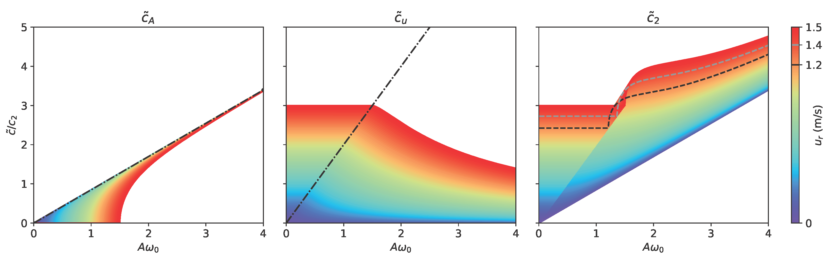
2. Theoretical Background

As discussed in [16], a general expression for the velocity-dependent fluid-induced damping force may be taken proportional to $\propto \left|{\dot{x}}^{n-1}\left(t\right)\right|\dot{x}\left(t\right)$, where $\dot{x}\left(t\right)$ is the structure velocity, and n is a non-negative integer. Some particular cases of this general expression are found for $n=0$, related to dry friction [17], while $n=2$ recovers the usual aerodynamic or hydrodynamic quadratic drag force [18]. The linear, or viscous, damping model is equivalent to setting $n=1$. Although the quadratic model is discussed in the context of very large structural deflections by [16], while the general case is extensively detailed by [19], in this work a simpler approach is followed based on energy considerations. This is particularly useful to make the connection between environmental conditions and structural motions in the context of floating wind turbines by assuming that the damping force is given by:

$$F_d\left(t\right)=c_1\dot{x}\left(t\right)+\frac{c_2}{u_0}|\dot{x}\left(t\right)-u_r|\left(\dot{x}\left(t\right)-u_r\right)$$

(1)

where $\dot{x}=\frac{\mathrm{d}x}{\mathrm{d}t}$ is the structure velocity, $u_r$ is the external flow velocity, and $c_i$ are the damping coefficients associated with the linear and nonlinear damping sources. Additionally, a characteristic velocity, $u_0$, has been introduced such that the dimensions of $c_1$ and $c_2$ are consistent. In what follows, this is assumed to be unity. The free equation of motion (without any external load) for a single degree of freedom with mass m may be written as:

$$\ddot{x}\left(t\right)=-{\omega }_0^{2}x\left(t\right)-\frac{F_d\left(t\right)}{m}$$

(2)

where ${\omega }_0=\sqrt{\frac{k}{m}}$ is the system’s undamped natural frequency, and $F_d\left(t\right)$ is the damping force, which may be a generic function of time, but here, it is assumed to be given by Equation (1).

For the linear damping model ($c_2=0$), the differential equation above has the well-known solution:

$$x\left(t\right)=A{e}^{-{\xi }_1{\omega }_{0}t}\cos \left({\omega }_0\sqrt{1-{\xi }_1^2}t+\varphi \right)=A{e}^{-{\xi }_1{\omega }_{0}t}\cos (w_{d}t+\varphi )$$

(3)

where ${\omega }_d={\omega }_0\sqrt{1-{\xi }_1^2}$ is the system damped frequency, $\varphi$ is the phase angle associated with the initial conditions, and ${\xi }_1$ is the damping ratio, defined as the ratio between the damping coefficient and its critical value as:

$${\xi }_1=\frac{c_1}{c_{cr}}=\frac{c_1}{2m{\omega }_0}$$

(4)

Although this is no longer true if $c_2\ne 0$, for low damping forces, one may still make some general considerations based on energy dissipated by the system over a full period, which may be written as:

$$W={\int }_T{F}_d\left(t\right)dx$$

(5)

Assuming the damping takes the form presented in Equation (1), for the linear damping contribution, one finds:

$$W_1=c_1{\int }_T\dot{x}\left(t\right)dx=c_1{\int }_T{\dot{x}}^{2}dt\approx c_1{A}^2{\omega }_0^2{\int }_T{\sin }^2\left({\omega }_{0}t\right)dt=c_1\left(A^2{\omega }_0\pi \right)$$

(6)

where it is assumed that to the first order, the motion may still be approximated over a full cycle as $x\left(t\right)=-A\cos \left({\omega }_{0}t\right)$, such that $\dot{x}=A{\omega }_0\sin \left({\omega }_{0}t\right)$. Under the same assumption, the nonlinear contribution, for the limiting case where $u_r=0$, may be obtained as:

$$\begin{array}{cc}\hfill W_2& =c_2{\int }_T\left|\dot{x}\right|\dot{x}dx=2c_2{\int }_{T/2}{\dot{x}}^{3}dt\approx 2c_2{A}^3{\omega }_0^3{\int }_{T/2}{\sin }^3\left({\omega }_{0}t\right)dt=\hfill \\ \hfill & =c_2\frac{8A^3{\omega }_0^2}{3}\hfill \end{array}$$

(7)

A straightforward comparison with the linear damping result unveils that the linear coefficient that best approximates the quadratic response in terms of energy dissipation, ${\tilde{c}}_2$, when expressed as a fraction of the damping coefficient $c_2$, is:

$$\frac{{\tilde{c}}_2}{c_2}=\frac{8}{3\pi }A{\omega }_0$$

(8)

From the expression above, it can be seen that for a purely quadratic damping force (meaning $u_r=0$), a linear dependency of the effective damping ratio on the motion amplitude is expected. Additionally, this dependency on the amplitude also implies that the identified value in an hypothetical experiment is not a direct measurement of the damping coefficient, its variation overtime being more relevant for this purpose.

Finally, the general nonlinear case with a nonvanishing external velocity ($u_r$) is more easily analysed if rewritten as:

$$\begin{array}{cc}\hfill \frac{W_2}{c_2}& ={\int }_T|\dot{x}-u_r|\left(\dot{x}-u_r\right)dx=\hfill \\ \hfill & =-{\int }_0^{T_1}{\left(\dot{x}-u_r\right)}^2\dot{x}dt+{\int }_{T_1}^{T_2}{\left(\dot{x}-u_r\right)}^2\dot{x}dt-{\int }_{T_2}^T{\left(\dot{x}-u_r\right)}^2\dot{x}dt=\hfill \\ \hfill & ={\int }_{T_1}^{T_2}{\left(\dot{x}-u_r\right)}^2\dot{x}dt-{\int }_{T_2}^{T+T_1}{\left(\dot{x}-u_r\right)}^2\dot{x}dt\hfill \end{array}$$

(9)

where $T_1$ and $T_2$ correspond to the lower and upper time limits of the region where the structural velocity is higher than the environmental one, meaning $\dot{x}=A{\omega }_0\sin \left({\omega }_{0}t\right)\ge u_r$ for $t\in [T_1,T_2]$. Solving the integrals leads to:

$$\begin{array}{cc}\hfill \frac{W_2}{c_2}& =-\frac{2A^3{\omega }_0^2}{3}\left[{\cos }^3\left(2\pi \frac{T_1}{T}\right)-{\cos }^3\left(2\pi \frac{T_2}{T}\right)-3\cos \left(2\pi \frac{T_1}{T}\right)+3\cos \left(2\pi \frac{T_2}{T}\right)\right]+\hfill \\ \hfill & +u_r{A}^2{\omega }_0\left[4\pi \left(\frac{1}{2}+\frac{T_1}{T}-\frac{T_2}{T}\right)-\sin \left(4\pi \frac{T_1}{T}\right)+\sin \left(4\pi \frac{T_2}{T}\right)\right]+\hfill \\ \hfill & -2u_r^{2}A\left[\cos \left(2\pi \frac{T_2}{T}\right)-\cos \left(2\pi \frac{T_1}{T}\right)\right]\hfill \end{array}$$

(10)

At this point, it is convenient to write the equivalent linear damping coefficient as:

$${\tilde{c}}_2={\tilde{c}}_A+{\tilde{c}}_u$$

(11)

where ${\tilde{c}}_A$ and ${\tilde{c}}_u$ include the terms proportional to the motion amplitude and to the environmental velocity, respectively, according to Equation (11) and that may be alternatively defined as:

$$\begin{array}{c}\hfill \frac{{\tilde{c}}_A}{c_2}=-\frac{2A{\omega }_0}{3\pi }\left[{\cos }^3\left({\omega }_0{T}_1\right)-{\cos }^3\left({\omega }_0{T}_2\right)-3\cos \left({\omega }_0{T}_1\right)+3\cos \left({\omega }_0{T}_2\right)\right]\end{array}$$

(12)

$$\begin{array}{cc}\hfill \frac{{\tilde{c}}_u}{c_2}& =\frac{u_r}{\pi }\left[2\left(\pi +{\omega }_0\left(T_1-T_2\right)\right)-\sin \left(2{\omega }_0{T}_1\right)+\sin \left(2{\omega }_0{T}_2\right)\right]\hfill \end{array}$$

$$\begin{array}{c}-\frac{2u_r^2}{A{\omega }_0\pi }\left[\cos \left({\omega }_0{T}_2\right)-\cos \left({\omega }_0{T}_1\right)\right]\hfill \end{array}$$

(13)

Additionally, two different situations should be analysed separately. Firstly, when $u_r>A{\omega }_0$, implying that $T_1=T_2=0$ and that the first integral in Equation (9) vanishes, the corresponding effective damping coefficients are:

$$\begin{array}{cc}\hfill & \frac{{\tilde{c}}_A}{c_2}=0\hfill \end{array}$$

(14)

$$\begin{array}{cc}\hfill & \frac{{\tilde{c}}_u}{c_2}=\frac{2\pi u_r{A}^2{\omega }_0}{A^2{\omega }_0\pi }=2u_r\hfill \end{array}$$

(15)

For $A{\omega }_0>u_r>0$, however, things are drastically different. In this case, $T_2={\displaystyle \frac{T}{2}}-T_1$, a condition that also implies $\cos \left({\omega }_0{T}_1\right)=-\cos \left({\omega }_0{T}_2\right)$ and $\sin \left({\omega }_0{T}_1\right)=\sin \left({\omega }_0{T}_2\right)$, and the same coefficients are now given by:

$$\begin{array}{cc}\hfill & \frac{{\tilde{c}}_A}{c_2}=\frac{4A^3{\omega }_0^2}{3A^2{\omega }_0\pi }\cos \left({\omega }_0{T}_1\right)\left[3-{\cos }^2\left({\omega }_0{T}_1\right)\right]=\frac{4A{\omega }_0}{3\pi }\left[\sqrt{1-\frac{u_r^2}{A^2{\omega }_0^2}}\left(2+\frac{u_r^2}{A^2{\omega }_0^2}\right)\right]\hfill \end{array}$$

(16)

$$\begin{array}{cc}\hfill & \frac{{\tilde{c}}_u}{c_2}=\frac{4u_r}{\pi }\left[{\omega }_0{T}_1+\frac{u_r}{A{\omega }_0}\cos \left({\omega }_0{T}_1\right)\right]=\frac{4u_r}{\pi }\left[{\sin }^{-1}\left(\frac{u_r}{A{\omega }_0}\right)+\frac{u_r}{A{\omega }_0}\sqrt{1-\frac{u_r^2}{A^2{\omega }_0^2}}\right]\hfill \end{array}$$

(17)

For completeness, it may be checked that for $u_r=0$, or, alternatively, for $A{\omega }_0\gg u_r$, one recovers:

$$\begin{array}{cc}\hfill & \frac{{\tilde{c}}_A}{c_2}=\frac{8}{3\pi }A{\omega }_0\hfill \end{array}$$

(18)

$$\begin{array}{cc}\hfill & \frac{{\tilde{c}}_u}{c_2}=0\hfill \end{array}$$

(19)

It may be noted that this is the same result as in [16], up to a different original definition of the damping coefficient.

The different contributions for the effective damping ratio of these systems, named after the conventions used in Equation (15), are presented in Figure 1 for different values of structural and environmental velocities, where a clear transition at $u_r=A{\omega }_0$ can be identified. It should be noted that the precise location of this transition depends on both the environmental conditions, here parameterised by $u_r$, and on the motion amplitude, such that in a general case, the structure may evolve from one regime to another. As may be seen, the amplitude-dependent contribution, given by ${\tilde{c}}_A$ on the left panel, is null for small amplitudes and rapidly converges to a velocity-independent value of $\frac{8}{3\pi }$ for characteristic structural velocities higher than the environmental one. On the other hand, the velocity-dependent contribution, given by ${\tilde{c}}_u$ in the centre panel, exhibits a constant value, but not null for low motion amplitudes, and decays above the critical velocity. An important aspect to retain is that, for a given environmental fluid velocity, $u_r$, the nonlinear damping contribution increases with the increasing motion amplitude. It is also true that for most of the amplitude range, the damping ratio increases with increasing fluid velocities. However, it is also possible to find conditions where the opposite happens, due to the sudden increase in the amplitude-dependent contribution. This effect is clear when the two dashed lines included in Figure 1 are compared. Finally, it can also be seen that for sufficiently small motion amplitude, or perhaps more importantly, for floating offshore wind platforms and for sufficiently small natural frequencies, the existence of sea current drastically changes the results. In fact, in the scenario of still water, a linear dependence on the motion amplitude is expected, while in the presence of currents, a constant damping force dictated by the current speed will appear.

3. Methods for Modal Identification

The identification of nonlinear systems is a large topic on its own, with several applications (see, for instance, [20]), but most modal identification methods are mostly based on the assumption that the structure behaviour is linear, or that at least the nonlinear response is subdominant and maybe safely neglected. Following the discussion in Section 2, this works tries to understand how these nonlinear terms impact the damping ratio estimates, when a linear method is used for the identification. For this purpose, a brief overview of the conventional logarithmic decay method is presented, as well as the traditional implementation of the SSI-COV.

3.1. Logarithmic Decay Method

For systems with linear damping, one may immediately see that the response is given by a periodic function modulated by a negative exponential, implying that ${\xi }_1$ can be directly evaluated from the response amplitude:

$$\ln \left(A{e}^{-{\xi }_1{\omega }_{0}t}\right)=\ln \left(A\right)-{\xi }_1{\omega }_{0}t$$

(20)

meaning that the envelope amplitude’s natural logarithm, here obtained through the peak value in every oscillation, is a linear function of time with slope $-{\xi }_1{\omega }_0$. As in [21,22], this idea can be generalised to define an equivalent damping at a given point as the time derivative of the slope that can be written, in general, as:

$$\xi ={\xi }_0+{\xi }_A$$

(21)

where ${\xi }_0$ and ${\xi }_A$ are the amplitude-independent and -dependent contributions. In the model under analysis, this relation may still be well approximated for most of the conditions as:

$$\xi ={\xi }_0+m_{\xi }·A$$

(22)

where A is the motion amplitude, and $m_{\xi }$ is a constant that depends on the damping regime: for a linear damping model or when $u_r<A{\omega }_0$, it is expected to vanish ($m_{\xi }\sim 0$), while for a nonlinear model and $u_r>A{\omega }_0$, it is expected to be given by $m_{\xi }\approx \frac{8{\omega }_0}{3\pi }{\xi }_2$, where ${\xi }_2$ should be interpreted as the dimensionless analogue of the nonlinear contribution:

$${\xi }_2=\frac{c_2}{2m{\omega }_0}$$

(23)

3.2. Stochastic Subspace Identification

If the method above is suitable to analyse the free-decay response of a given structure, it fails to properly characterise the response under a stochastic action and/or when more than one mode contributes to the response. If the latter can be mitigated by a suitable application of data-filtering methodologies, the former requires more robust and sophisticated approaches. In this work, the SSI-COV method (covariance-driven stochastic subspace identification), applied for the first time in [11] in the context of structural identification, was used. This methodology is based on the identification of a state-space model [23] of the recorded response (${\mathit{y}}_k$) as:

$$\begin{array}{cc}\hfill & {\mathit{x}}_{k+1}=\mathit{A}·{\mathit{x}}_k+{\mathit{w}}_k\hfill \end{array}$$

(24)

$$\begin{array}{cc}\hfill & {\mathit{y}}_k=\mathit{C}·{\mathit{x}}_k+{\mathit{v}}_k\hfill \end{array}$$

(25)

where ${\mathit{x}}_k$ is the state vector, and ${\mathit{w}}_k$ and ${\mathit{v}}_k$ the process and measurement noise, respectively, and where the state matrix $\mathit{A}$ contains all the relevant dynamic information of the system. The critical step for the method is the identification, under a white-noise external action, of the state matrix from the output correlation matrix, using equations [23]:

$${\mathit{R}}_y\left(j\right)=E\left[{\mathit{y}}_{k+j}·{\mathit{y}}_k^T\right]=\mathit{C}·{\mathit{A}}^{j-1}·\mathit{G}=\mathit{C}·{\mathit{A}}^{j-1}·E\left[{\mathit{x}}_{k+1}·{\mathit{y}}_k^T\right]$$

(26)

which allows us to distribute the correlation matrices in a Toeplitz matrix such that:

$$\begin{array}{cc}\hfill {\mathit{T}}_{\left(1\right|j_i)}& =\left[\begin{array}{cccc}{\mathit{R}}_{ji}^{ref}& {\mathit{R}}_{ji-1}^{ref}& \cdots & {\mathit{R}}_1^{ref}\\ {\mathit{R}}_{ji+1}^{ref}& {\mathit{R}}_{ji}^{ref}& \cdots & {\mathit{R}}_2^{ref}\\ ⋮& ⋮& \ddots & ⋮\\ {\mathit{R}}_{2·ji-1}^{ref}& {\mathit{R}}_{2·ji-2}^{ref}& \cdots & {\mathit{R}}_{ji}^{ref}\end{array}\right]=\left[\begin{array}{c}\mathit{C}\\ \mathit{C}·\mathit{A}\\ ⋮\\ \mathit{C}·{\mathit{A}}^{j_i-1}\end{array}\right]·\left[\begin{array}{cccc}{\mathit{A}}^{j_i-1}·\mathit{G}& \cdots & \mathit{A}·\mathit{G}& \mathit{G}\end{array}\right]\hfill \\ \hfill & =\left[\begin{array}{cc}{\mathit{U}}_1& {\mathit{U}}_2\end{array}\right]·\left[\begin{array}{cc}{\mathit{S}}_1& \mathbf{0}\\ \mathbf{0}& \mathbf{0}\end{array}\right]·\left[\begin{array}{c}{\mathit{V}}_1^T\\ {\mathit{V}}_2^T\end{array}\right]\hfill \end{array}$$

(27)

where the last equality follows from the singular value decomposition of the Toeplitz matrix, and the non-zero values of this decomposition are marked with the index 1. The Toeplitz matrix can still be written from the observability ($\mathit{O}$) and controllability ($\mathbf{\Gamma }$) matrices as:

$$\left\{\begin{array}{c}{\mathit{O}}_{j_i}={\mathit{U}}_1·{\mathit{S}}_1^{\frac{1}{2}}\hfill \\ {\mathbf{\Gamma }}_{j_i}={\mathit{S}}_1^{\frac{1}{2}}·{\mathit{V}}_1^T\hfill \end{array}\right.⟶{\mathit{T}}_{\left(1\right|j_i)}={\mathit{O}}_{j_i}·{\mathbf{\Gamma }}_{j_i}$$

(28)

Comparing Equations (27) and (28), it can be easily shown that the output matrix $\mathit{C}$ can be computed from the first n lines of the observability matrix, n being the number of DOFs of the system. Having defined the output matrix, the corresponding state matrix results from an optimisation problem since († stands for the Moore–Penrose pseudoinverse matrix):

$$\left[\begin{array}{c}\mathit{C}\\ \mathit{C}·\mathit{A}\\ ⋮\\ \mathit{C}·{\mathit{A}}^{j_i-2}\end{array}\right]·\mathit{A}=\left[\begin{array}{c}\mathit{C}·\mathit{A}\\ \mathit{C}·{\mathit{A}}^2\\ ⋮\\ \mathit{C}·{\mathit{A}}^{j_i-1}\end{array}\right]⟶\mathit{A}={\left[\begin{array}{c}\mathit{C}\\ \mathit{C}·\mathit{A}\\ ⋮\\ \mathit{C}·{\mathit{A}}^{j_i-2}\end{array}\right]}^{†}·\left[\begin{array}{c}\mathit{C}·\mathit{A}\\ \mathit{C}·{\mathit{A}}^2\\ ⋮\\ \mathit{C}·{\mathit{A}}^{j_i-1}\end{array}\right]$$

(29)

Having identified the state matrix, the mode shapes’ components, natural frequencies and modal damping ratios follow directly from its eigendecomposition [24]:

$$\mathit{A}=\mathbf{\Psi }·{\mathbf{\Lambda }}_D·{\mathbf{\Psi }}^{-1}$$

(30)

where $\mathbf{\Psi }$ contains the mode shapes’ components in its columns, and ${\mathbf{\Lambda }}_D$ is diagonal with the discrete-time eigenvalues (${\mu }_k$), related to the natural frequencies (${\omega }_k$) and modal damping coefficients (${\xi }_k$) by [24]:

$$\left\{\begin{array}{c}{\lambda }_k=\frac{\ln {\mu }_k}{\Delta t}\hfill \\ {\lambda }_k,{\lambda }_k^{*}=-{\xi }_k·{\omega }_k\pm i·\sqrt{1-{\xi }_l^2}·{\omega }_k\hfill \end{array}\right.⟶\left\{\begin{array}{c}{\omega }_k=\left|{\lambda }_k\right|\hfill \\ {\xi }_k=-\frac{\Re \mathrm{e}\left({\lambda }_k\right)}{|{\lambda }_k|}\hfill \end{array}\right.$$

(31)

When real observation data are used, the number of non-zero singular values of the Toeplitz matrix, or model order, is not clearly defined, as a significant number of poles may be needed to properly model the noise and the load frequency content induced in the response. As this value is a priori unknown, a common procedure in operational modal analysis is to test different model orders, keeping only the modes that are consistently obtained, regardless of the order used. In this work, we also introduce a new criterion for modal differentiation that explores the amplitude of the modes identified in the state matrix decomposition. Although this information is often not considered since the mode shapes are only defined up to a numerical factor, in real applications where the state matrix is obtained from experimental data, the retrieved configurations have imprinted the level of excitation of each mode. It may be argued that this effect also reflects the modal coordinate at a given point, but from an identification point of view, both aspects are completely degenerated and cannot be immediately distinguished.

Finally, it should also be noted that while the SSI-COV method was originally developed as a tool for stochastic identification, it also relies on the fact that the observed free decays are closely related with the correlations of the responses associated with a white-noise excitation. Consequently, measured free decays can also be used as input to the SSI-COV method, taking the place of the correlation functions calculated from the ambient responses [25]. In this case, instead of basing the identification on the correlations between the measured responses, the algorithm is applied to a time-dependent matrix with a single column containing the free decays measured at the instrumented points. If this approach solves the already mentioned limitation of the traditional procedure based on the logarithmic decrement of the response that requires the contribution of a single mode to be isolated, eventually, by the application of band-pass filters, it should be noted that the amplitude-dependence identification of the damping coefficient is, at least, partially lost.

4. Simplified Single Degree of Freedom Model

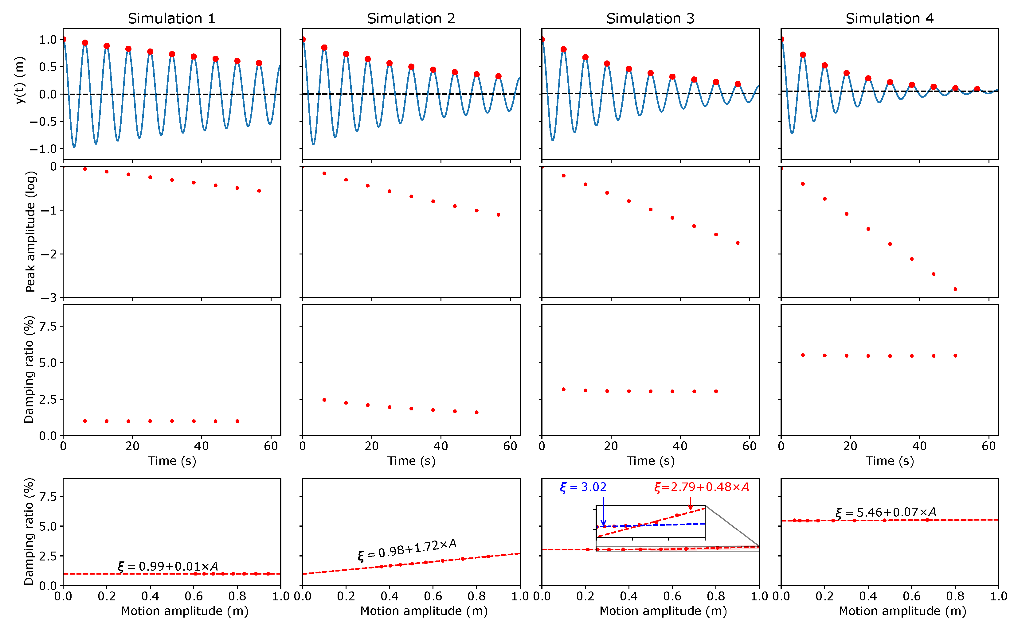
In the previous section some analytical predictions were derived for the effective energy dissipation induced by hydrodynamic and aerodynamic responses, or more generally, by any nonlinear damping source that may be parameterised by Equation (1). To see how they stand against numerically simulated data, the equation of motion was numerically evaluated for different conditions considering the following model parameters:

• Simulation 1: ${\xi }_1=1\%$, ${\xi }_2=0\%$, $u_r=0$ m/s
• Simulation 2: ${\xi }_1=1\%$, ${\xi }_2=2\%$, $u_r=0$ m/s
• Simulation 3: ${\xi }_1=1\%$, ${\xi }_2=2\%$, $u_r=0.5$ m/s
• Simulation 4: ${\xi }_1=1\%$, ${\xi }_2=2\%$, $u_r=1.1$ m/s

The values above were defined in order to cover the different damping regimes discussed in Section 2, here expressed in terms of the damping ratio ${\xi }_1$ and ${\xi }_2$. Without loss of generality, it was assumed in all simulations that ${\omega }_0=1$.

4.1. Free-Decay Analysis

In a first approach, the response was simulated by imposing a unitary initial displacement and null velocity as initial conditions. For each simulation, the free decay was analysed and the damping ratio estimated based on the logarithmic decrement at every two periods. The results are presented in Figure 2, where some relevant aspects that confirm the theoretical predictions can be identified.

Firstly, for the linear damping case, a constant equivalent damping is identified and the original value recovered, which should come as no surprise since this is just a simple linearly damped harmonic oscillator whose behaviour is well understood. In the second case, however, a clear linear trend can be seen, as predicted from the quadratic force. In this case, it can be checked that the interception at the origin is given by the linear damping coefficient once more, while the amplitude-dependent slope is well approximated by $\frac{8}{3\pi }{\xi }_2\approx 1.70\%$. Finally, the two simulations where an external flow velocity was considered also exhibit the expected characteristic features. On one hand, for velocities higher than the structural peak velocity, the results are well approximated by a single, constant, equivalent damping coefficient given by $\tilde{\xi }\approx {\xi }_1+2u_r{\xi }_2=1+2\times 1.1\times 2=5.4\%$. On the other hand, Simulation 3 shows the phase transition happening at $u_r=A{\omega }_0$. In this case, this threshold is achieved midway through the simulation and at posterior times (associated with lower motion amplitudes), the solution is once more well approximated by a constant equivalent damping, here given by $\tilde{\xi }\approx {\xi }_1+2u_r{\xi }_2=1+2\times 0.5\times 2=3\%$.

The free decays for the different simulations were used as input to the SSI-COV algorithm, and the results obtained are presented in Figure 3, where a reference value based on the free decay results just described has also been included for reference as a dashed line, based on the different limits that are adequate for each simulation. Here, and in the following, the SSI-COV results are presented as stabilisation diagrams: the first row includes the different stable poles (a pole is considered stable if the frequency and damping variation between model orders is not higher than 1% and 10%, respectively) identified for different model orders, with the corresponding damping level and the relative contribution for the total response presented on the second and third row, respectively. The poles were separated in different clusters with DBSCAN [26] using as metric the differences in the frequency, damping and modal contribution. It is interesting to note that while the results from Simulation 1 trivially recover the theoretical values, the remaining simulations exhibit different properties. In fact, it can be seen that Simulation 2, where the environmental velocity vanishes, corresponds to the cases where the identification is harder and exhibits significant scatter. On the other hand, as the environmental velocity increases, the natural frequency identification is easily recovered, but different harmonics are also found. These harmonics, due to the nonlinear components of the model, are also partially visible in Simulation 2.

Finally, it can still be seen that the introduced criteria regarding the modal contribution as estimated from the decomposition of the Toeplitz matrix can be used to effectively identify the relevant modes for the identification.

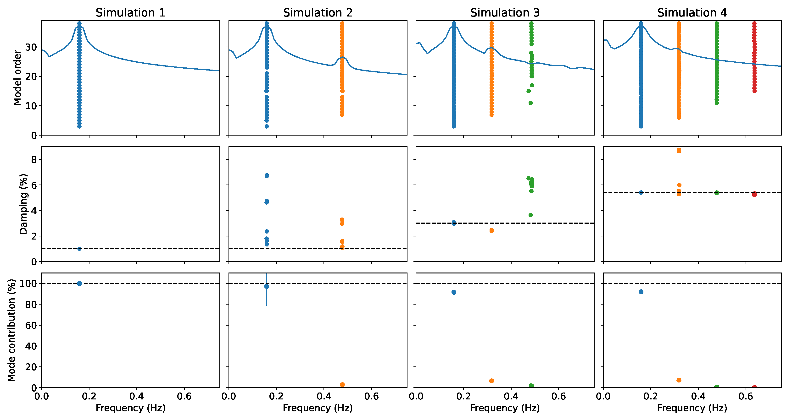
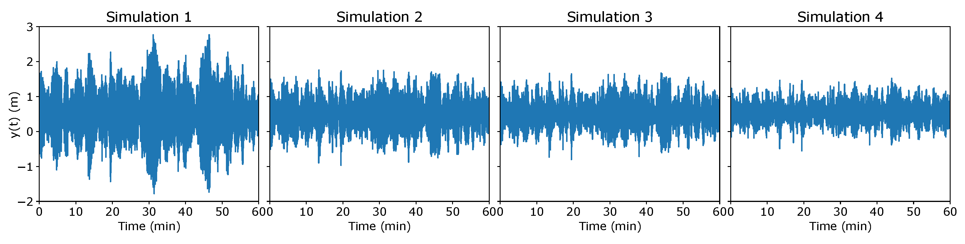
4.2. Stochastic Excitation

If the results until now were already expected based on the theoretical considerations previously presented, they also clearly identify the possible issues for output-only identification methods, where a linear structural behaviour is assumed. In particular, the SSI-COV algorithm strictly depends on this assumption through, at least, two different perspectives. Firstly, the method inputs are the correlation functions that are obtained by averaging over the full time series. If the system undergoes a nonlinear motion, this averaging procedure will inevitably fail. On the other hand, and even considering that the free decay could be well defined, for instance by using free-decay test results such as the ones presented in Figure 2, the method characterises the state matrix of what is assumed to be a linear system, a condition that is once more not verified.

If the issues above could raise the question of whether or not to use the SSI-COV, the fact is that the free decays that have been used as a direct input for the identification method are not compatible with the more commonly available experimental data. To emulate this situation, the single-degree-of-freedom model was excited with a white-noise external action for 4000 s. The generated time series after removing the first 400 s to ensure that the transient events were properly faded away are presented in Figure 4. The results of the SSI-COV method are presented in Figure 5, where 30 s was used for the length of the correlation function estimates. Once more, it can be seen that in all cases, the estimated damping coefficient is in accordance with the values obtained for the free decay, but different for different environmental conditions (note that all simulations were conducted with the same structural properties). Additionally, while Simulations 1, 3 and 4 recover the expected theoretical values, Simulation 2, where the amplitude dependence of the response was more pronounced, exhibits a higher scatter in the damping estimates. In all cases but Simulation 1, it should be noted that the identified value is not a direct estimate of the damping coefficient.

Additionally, the constant and stable values found in all simulations for the damping ratio may come as a hint that the induced motion amplitudes are mostly falling below the threshold previously identified. To test this hypothesis, the response was simulated for different intensities of white-noise loading. The evolution of the identified damping ratio with the characteristic motion amplitude, as defined by its standard deviation, is presented in Figure 6. The motion amplitude was used rather than the white-noise characteristic value, since it is expected to be more closely related to the identified damping ratio. As can be seen, while Simulation 1’s predictions are stable for arbitrary conditions, as expected, Simulation 2 to 4 exhibit a clear dependency on the intensity of the external loading. In fact, it can be seen that there is a given characteristic motion amplitude that separates a region where the identified damping is constant from a region where it increases with the motion amplitude. Additionally, it can be seen that the point at which this transition is found is closely related to the reference environmental speed, $u_r$, of the corresponding simulation: in Simulation 2, $u_r=0$ and the amplitude dependence is found for all simulated conditions, in Simulation 3 and 4, with $u_r\ne 0$, a constant damping coefficient is found for motion amplitudes ∼$u_r$, increasing after that threshold (note that the theoretical prediction is found at $A{\omega }_0$, but here, ${\omega }_0=1$, and A is closely related with the motion’s standard deviation).

5. Numerical Validation with Full Aeroelastic Simulations

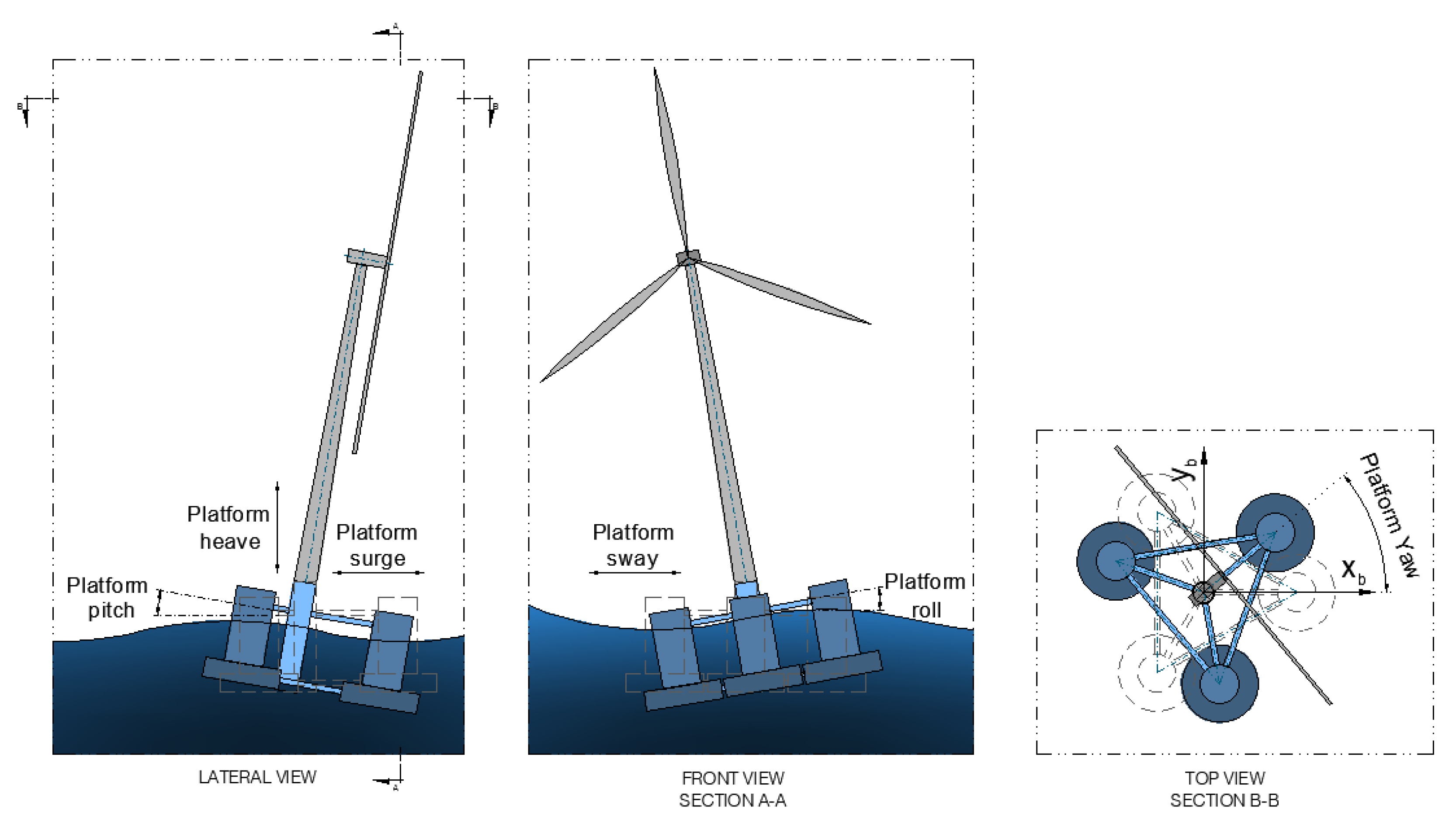
5.1. Numerical Model Description

Having studied the impact of different damping models on the performance of output-only identification methods, in the following section, this is used to gain insight into data that more closely mimic experimental records. For this purpose, the NREL 5 MW wind turbine [27] and the corresponding reference semisubmersible floating platform designed for Phase II of the Offshore Code Comparison 4 (OC4) [28] were used to simulate the dynamic response for different environmental and operation conditions. It should be noted that in this case, two different sources of nonlinear damping were present, the hydrodynamic and aerodynamic counterparts, which differently impacted the surge and pitch motions of the floating platform. In all simulations where a turbulent wind field was considered, the full wind field was generated using NREL’s TurbSim [29] generator with a varying reference mean wind speed and turbulence intensity. The mooring systems were modelled using MoorDyn [30]. While the platform motions are typically described from three translations (surge, sway and heave) and three rotations around the same axis (roll, pitch and yaw), as represented in Figure 7, in this work, for the sake of brevity, the evaluation of the SSI-COV performance was made using as input for the algorithm the platform surge and pitch motions as output by OpenFAST. For reference, these motions were associated with a natural frequency of 0.009 Hz and 0.037 Hz, respectively [28,31].

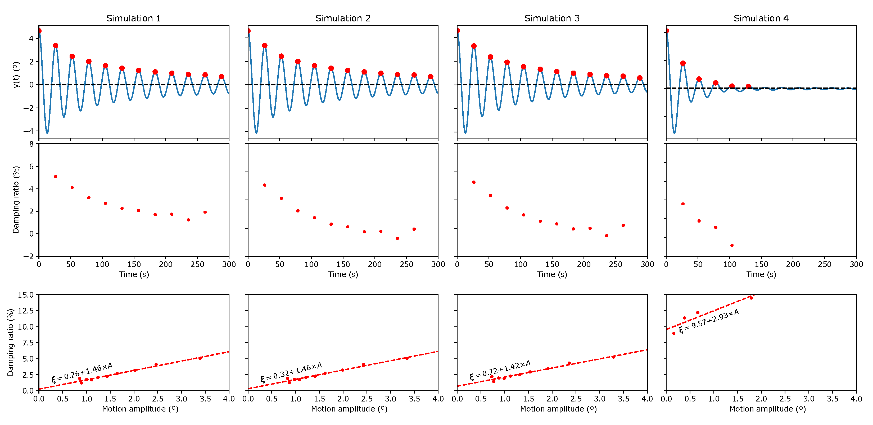
5.2. Free-Decay Analysis

As a first step, the structure was displaced from its equilibrium position and the corresponding free decay evaluated. This work focused on the surge motion, by imposing a 10 m displacement along this direction, and the pitch motion, by imposing a 5° rotation along the relevant axis. For each case, the free decay was computed for the following environmental conditions:

• Simulation 1: reference scenario without currents nor wind;
• Simulation 2: sea current with a velocity of 0.25 m/s, no wind;
• Simulation 3: 3 m/s steady wind field, parked rotor;
• Simulation 4: 22 m/s steady wind field, normal-operation rotor with a constant angular velocity of 12.1 RPM (revolutions per minute).

In all simulations, the pitch value was defined to be 20°. The higher wind speed was chosen from [27] as the normal operation conditions associated with the same pitch angle and the rotor angular velocity was set for the corresponding value of 12.1 RPM. Finally, since in all simulations but Simulation 1, the structure is displaced from its equilibrium position by wind or current loading, a preliminary simulation without the prescribed displacement was conducted, and the new equilibrium position used as initial conditions for the free-decay analysis. This procedure ensured that the free decay was performed with exactly the same initial conditions in all cases. The results based on the logarithmic decrement are presented in Figure 8 and Figure 9 for the surge and pitch motions, respectively. It may be easily seen that the surge motion is mostly impacted by the presence of a nonvanishing current rather than by the external wind field. On the other hand, the pitch motion is strongly impacted by the wind speed, but not by the current. This can be explained from the fact that the structure velocity at the rotor level sourced by the pitch motion is not only associated with higher frequencies (when compared with surge motion) but is also amplified by the tower height. At this point, it should be mentioned that although Simulation 4 was compatible with normal operation conditions, the controllers were not active, implying that both the rotor angular velocity and the blades’ pitch angle were constant throughout the simulation time. In a more realist scenario, the velocity variation sourced by the pitch motion would trigger a response from the control system that would impact the results. Although this is clearly an oversimplification, this analysis should not be understood as representative of actual operating conditions (it is not expected to conduct a free-decay analysis with an operating rotor in the first place) but to illustrate the impact of the different contributions for the overall damping level of the different motions.

Once more, the same results could be estimated using the SSI-COV and the results are presented, for reference, for the surge motion in Figure 10, where the presence of the fundamental frequency harmonics is easily identified. This is important because it unveils that this effect can be used to identify nonlinear contributions that could be otherwise interpreted as independent modes. It may also be seen that the identified damping levels exhibit a significant scatter, except for Simulation 2. This can be understood, since the case with the external sea current is the one where the damping level is dominated by the amplitude-independent terms. In all other cases, there is a pronounced dependence on the motion amplitude, and this is perceived as different damping levels in the stabilisation diagrams. In fact, and referring back to Figure 8, it may be seen that the scatter is compatible with the maximum and minimum damping levels identified in the logarithmic decay analysis.

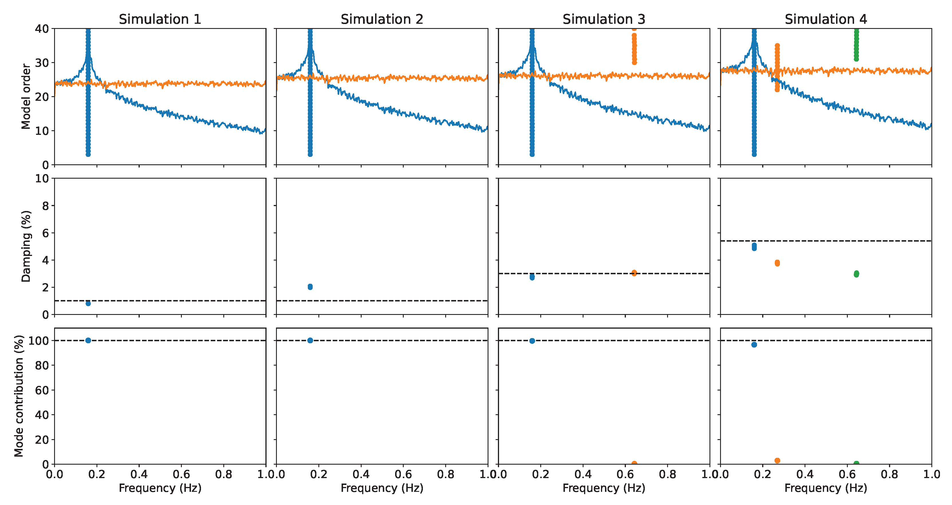
5.3. Stochastic Excitation

Finally, the structural response with a stochastic wind field characterised by a given wind speed and turbulence intensity was simulated. To avoid including transient effects associated with the model convergence in the first time steps, the results were obtained by running 4000 s simulations and discarding the first 400 s, leaving 3600 s (60 min) for the data analysis. For simplicity, no wave loading was considered in the simulations, implying that the stochastic nature of the response was fully characterised by the wind field’s turbulent component. Since the damping level was expected to depend on the motion amplitude (essentially conditioned by the wind turbulence) as well as on the average wind speed, the following 3D wind fields were generated:

• Wind field 1: 2.5 m/s mean wind speed with a 10% turbulence intensity;
• Wind field 2: 2.5 m/s mean wind speed with a 26% turbulence intensity;
• Wind field 3: 6.5 m/s mean wind speed with a 10% turbulence intensity.

Note that the chosen conditions ensured that the standard deviation of the wind time series was the same in wind field 2 and wind field 3. All conditions were combined with different sea current velocities between 0 and 50 cm/s, for a total of 33 independent simulations. The stabilisation diagrams for the minimum and maximum current speeds considered, as well as an intermediate case, are presented in Figure 11 for wind field 1. As can be seen, the damping level associated with the surge motion seems to increase with the speed of the current, while the same does not seem to happen for the pitch motion.

The identified damping ratio evolution with the current and wind speed is presented in Figure 12 for the studied surge and pitch motion. As can be seen, neither the average speed nor the energy associated with the turbulent component of the wind field seems to significantly impact the identified damping for surge motion, which is completely dominated by the sea current intensity. This is an expected result following the free-decay analysis, since the energy dissipation for this particular motion was found to be associated with the hydrodynamic response. On the other hand, the pitch motion was found to be mostly governed by the aerodynamic damping at the rotor level, and this was also confirmed by the simulations. In fact, it can be seen that the current intensity does not impact significantly the damping level identified, which now can be seen to be more correlated to the mean wind speed. It can also be seen that the energy content associated with the turbulent components also contribute to higher damping levels, even considering that the simulations’ conditions were associated with small-amplitude pitch rotations.

6. Conclusions

In this work, the applicability of the output-only method SSI-COV for modal identification in the presence of nonlinear damping sources was discussed, with a particular focus on the relation between the identified damping level and the corresponding linear and nonlinear damping coefficients. In a first approach, based solely on an analytical analysis and energy dissipation considerations, it was shown that the equivalent damping ratio that this type of systems experience depends on the relation between the characteristic motion amplitude and the external (environmental) reference velocity, with a motion’s frequency-dependent critical value separating two distinct regions. This behaviour shows that the relation between identified damping ratio and the structure damping coefficients is not trivial, which is an important conclusion when calibrating numerical models with experimental data.

In a second step, the theoretical predictions were verified by numerically solving the equation of motion of a single-degree-of-freedom system for a single initial perturbation and with a stochastic excitation. If in the first case, the variation in the damping ratio with the motion amplitude becomes evident, the same does not happen when methods for stochastic identification are required. In these cases, it was shown that additional harmonics of the fundamental frequency appear in the stabilisation diagram. These should not be taken as additional structural modes.

Finally, the gained insight was used to better understand the results and damping levels using a full hydro-aeroelastic simulation of a reference floating wind turbine for different sea currents and wind field properties. This analysis showed that the damping level of different platform motions is impacted differently by the different environmental conditions. Here, a remark should be made, since only very particular conditions were tested, where the wind turbine rotor was either parked or spinning with a constant angular velocity. The study of the control system’s impact on the results is left for future work.

References

1. Magalhães, F.; Cunha, A. Explaining operational modal analysis with data from an arch bridge. Mech. Syst. Signal Process. 2011, 25, 1431–1450. [Google Scholar] [CrossRef]
2. Zhang, L.; Brincker, R. An Overview of Operational Modal Analysis: Major Development and Issues. In Proceedings of the International Modal Analysis Conference, Copenhagen, Denmark, 26–27 April 2005. [Google Scholar]
3. Rainieri, C.; Fabbrocino, G. Output-only Modal Identification BT. In Operational Modal Analysis of Civil Engineering Structures: An Introduction and Guide for Applications; Springer: New York, NY, USA, 2014; pp. 103–210. [Google Scholar] [CrossRef]
4. Devriendt, C.; Magalhães, F.; Weijtjens, W.; Sitter, G.D.; Cunha, A.; Guillaume, P. Structural health monitoring of offshore wind turbines using automated operational modal analysis. Struct. Health Monit. 2014, 13, 644–659. [Google Scholar] [CrossRef]
5. Weijtjens, W.; Verbelen, T.; De Sitter, G.; Devriendt, C. Foundation structural health monitoring of an offshore wind turbine—A full-scale case study. Struct. Health Monit. 2015, 15, 389–402. [Google Scholar] [CrossRef]
6. Xu, M.; Au, F.T.K.; Wang, S.; Wang, Z.; Peng, Q.; Tian, H. Dynamic response analysis of a real-world operating offshore wind turbine under earthquake excitations. Ocean Eng. 2022, 266, 112791. [Google Scholar] [CrossRef]
7. Hines, E.M.; Baxter, C.D.P.; Ciochetto, D.; Song, M.; Sparrevik, P.; Meland, H.J.; Strout, J.M.; Bradshaw, A.; Hu, S.L.; Basurto, J.R.; et al. Structural instrumentation and monitoring of the Block Island Offshore Wind Farm. Renew. Energy 2023, 202, 1032–1045. [Google Scholar] [CrossRef]
8. Ruzzo, C.; Failla, G.; Collu, M.; Nava, V.; Fiamma, V.; Arena, F. Operational Modal Analysis of a Spar-Type Floating Platform Using Frequency Domain Decomposition Method. Energies 2016, 9, 870. [Google Scholar] [CrossRef]
9. Ruzzo, C.; Failla, G.; Collu, M.; Nava, V.; Fiamma, V.; Arena, F. Output-only identification of rigid body motions of floating structures: A case study. Procedia Eng. 2017, 199, 930–935. [Google Scholar] [CrossRef]
10. Pimenta, F.; Ribeiro, D.; Román, A.; Magalhães, F. Modal properties of floating wind turbines: Analytical study and operational modal analysis of an utility-scale wind turbine. Eng. Struct. 2024, 301, 117367. [Google Scholar] [CrossRef]
11. Peeters, B.; De Roeck, G. Reference-based stochastic subspace identification for output-only modal analysis. Mech. Syst. Signal Process. 1999, 13, 855–878. [Google Scholar] [CrossRef]
12. Van Overschee, P.; De Moor, B. Subspace Identification for Linear Systems: Theory, Implementation, Applications; Springer: New York, NY, USA, 2012. [Google Scholar]
13. Falzarano, J.M.; Clague, R.E.; Kota, R.S. Application of Nonlinear Normal Mode Analysis to the Nonlinear and Coupled Dynamics of a Floating Offshore Platform with Damping. Nonlinear Dyn. 2001, 25, 255–274. [Google Scholar] [CrossRef]
14. Liagre, P.F.; Niedzwecki, J.M. Estimating nonlinear coupled frequency-dependent parameters in offshore engineering. Appl. Ocean Res. 2003, 25, 1–19. [Google Scholar] [CrossRef]
15. Al-hababi, T.; Cao, M.; Saleh, B.; Alkayem, N.F.; Xu, H. A Critical Review of Nonlinear Damping Identification in Structural Dynamics: Methods, Applications, and Challenges. Sensors 2020, 20, 7303. [Google Scholar] [CrossRef] [PubMed]
16. Colin, M.; Thomas, O.; Grondel, S.; Cattan, E. Very large amplitude vibrations of flexible structures: Experimental identification and validation of a quadratic drag damping model. J. Fluids Struct. 2020, 97, 103056. [Google Scholar] [CrossRef]
17. Géradin, M.; Rixen, D.J. Mechanical Vibrations: Theory and Application to Structural Dynamics; John Wiley & Sons: Hoboken, NJ, USA, 2014. [Google Scholar]
18. Anderson, J.D. Fundamentals of Aerodynamics, 6th ed.; Aeronautical and Aerospace Engineering Series; McGraw-Hill: New York, NY, USA, 2001. [Google Scholar]
19. Elliott, S.J.; Tehrani, M.G.; Langley, R.S. Nonlinear damping and quasi-linear modelling. Philos. Trans. R. Soc. A Math. Phys. Eng. Sci. 2015, 373, 20140402. [Google Scholar] [CrossRef] [PubMed]
20. Kerschen, G.; Worden, K.; Vakakis, A.F.; Golinval, J.C. Past, present and future of nonlinear system identification in structural dynamics. Mech. Syst. Signal Process. 2006, 20, 505–592. [Google Scholar] [CrossRef]
21. Jeary, A.P. Damping in tall buildings—A mechanism and a predictor. Earthq. Eng. Struct. Dyn. 1986, 14, 733–750. [Google Scholar] [CrossRef]
22. Jeary, A.P. The description and measurement of nonlinear damping in structures. J. Wind Eng. Ind. Aerodyn. 1996, 59, 103–114. [Google Scholar] [CrossRef]
23. Overschee, P.V.; Moor, B.D. Subspace Identification for Linear Systems; Kluwer Academic Publishers: Leuven, Belgium, 1996. [Google Scholar]
24. Quallen, S.; Xing, T. CFD simulation of a floating offshore wind turbine system using a variable-speed generator-torque controller. Renew. Energy 2016, 97, 230–242. [Google Scholar] [CrossRef]
25. Magalhães, F. Operational Modal Analysis for Testing and Monitoring of Bridges and Special Structures. Ph.D. Thesis, Faculty of Engineering of the University of Porto, Porto, Portugal, 2010. [Google Scholar]
26. Ester, M.; Kriegel, H.P.; Sander, J.; Xu, X. A density-based algorithm for discovering clusters in large spatial databases with noise. In Proceedings of the Second International Conference on Knowledge Discovery and Data Mining, Portland, OR, USA, 2–4 August 1996; KDD’96. pp. 226–231. [Google Scholar]
27. Jonkman, J.; Butterfield, S.; Musial, W.; Scott, G. Definition of a 5-MW Reference Wind Turbine for Offshore System Development; Technical Report 38060; National Renewable Energy Lab. (NREL): Golden, CO, USA, 2009. [Google Scholar] [CrossRef]
28. Robertson, A.; Jonkman, J.; Masciola, M.; Song, H.; Goupee, A.; Coulling, A.; Luan, C. Definition of the Semisubmersible Floating System for Phase II of OC4; Technical Report 60601; National Renewable Energy Lab. (NREL): Golden, CO, USA, 2014. [Google Scholar] [CrossRef]
29. Jonkman, B.J.; Buhl, M.L., Jr. TurbSim User’s Guide; Technical Report 39797; National Renewable Energy Laboratory: Golden, CO, USA, 2006. [Google Scholar]
30. Hall, M. MoorDyn User’s Guide; Technical Report; Department of Mechanical Engineering, University of Maine: Orono, ME, USA, 2015. [Google Scholar]
31. Pimenta, F.; Ruzzo, C.; Failla, G.; Arena, F.; Alves, M.; Magalhães, F. Dynamic Response Characterization of Floating Structures Based on Numerical Simulations. Energies 2020, 13, 5670. [Google Scholar] [CrossRef]
Figure 1. Evolution of the different contributions, as defined in Equation (9), for the effective damping of the structure expressed with respect to the true damping coefficient, c 2 . In the left panel, the amplitude-dependent term, c ˜ A , with the limit defined by Equation (18) included as dashed-dotted line. In the centre panel, the external velocity-dependent contribution, c ˜ u , with the limit defined by Equation (15) for A ω 0 = u r indicated as dashed-dotted line. In the right panel, the total effective damping, obtained as a superposition of the two contributions from the previous panels. In this case, the dashed lines are included for two particular values of u r = 1.2 m/s and u r = 1.4 m/s.
Energies 17 01671 g001
Figure 2. Identified damping coefficients from a free decay for different combinations of linear and nonlinear damping sources based on the logarithmic decay.
Energies 17 01671 g002
Figure 3. Stabilisation diagrams obtained with SSI-COV using the free decay for different combinations of linear and nonlinear damping sources as direct inputs.
Energies 17 01671 g003
Figure 4. System response when subjected to a stochastic loading for different combinations of linear and nonlinear damping sources.
Energies 17 01671 g004
Figure 5. Stabilisation diagrams obtained with SSI-COV using the correlation functions estimated from the stochastic response of the system for different combinations of linear and nonlinear damping sources.
Energies 17 01671 g005
Figure 6. Evolution of the identified damping ratio for different intensity stochastic loading in the different simulation scenarios.
Energies 17 01671 g006
Figure 7. Rigid body’s degrees of freedom of a floating offshore wind turbine.
Energies 17 01671 g007
Figure 8. Identified damping coefficients from a free decay for different combinations of wind and current conditions for the surge motion.
Energies 17 01671 g008
Figure 9. Identified damping coefficients from a free decay for different combinations of wind and current conditions for the pitch motion.
Energies 17 01671 g009
Figure 10. Stabilisation diagrams obtained with SSI-COV using the surge’s free decay for different combinations of environmental conditions (poles associated with the surge’s fundamental frequency in blue).
Energies 17 01671 g010
Figure 11. Stabilisation diagram for the case without current (on the left), for a 25 cm/s current (middle panel) and a 50 cm/s current (on the right). The relevant poles for the surge and pitch motion are coloured in blue and orange, respectively.
Energies 17 01671 g011
Figure 12. Evolution of the damping ratio as a function of the current speed and the wind field properties for surge and pitch motions. On the left panel are presented the stable poles’ damping and frequency values obtained for the relevant motions and all the setups.
Energies 17 01671 g012
Disclaimer/Publisher’s Note: The statements, opinions and data contained in all publications are solely those of the individual author(s) and contributor(s) and not of MDPI and/or the editor(s). MDPI and/or the editor(s) disclaim responsibility for any injury to people or property resulting from any ideas, methods, instructions or products referred to in the content.