Abstract
Predicting the remaining useful life (RUL) of lithium-ion batteries is crucial for enhancing their reliability and safety. Addressing the issue of inaccurate RUL predictions caused by the nonlinear decay resulting from capacity regeneration, this paper proposes an indirect lithium-ion battery RUL prediction method based on complete ensemble empirical mode decomposition with adaptive noise (CEEMDAN) and convolutional neural network (CNN)–bidirectional gated recurrent unit (BiGRU). The method extracts Health Indicators (HI) from the battery-charging stage and employs CEEMDAN to decompose HI into several components. These components are then input into a component prediction model for forecasting. Finally, the predicted component results are fused and input into a capacity prediction model to achieve indirect RUL prediction. Validation is conducted using the lithium-ion battery dataset provided by NASA. The results indicate that, under prediction starting points (STs) of 80 and 100, the maximum average absolute errors do not exceed 0.0096 and 0.0081, and the maximum root mean square errors do not exceed 0.0196 and 0.0115, demonstrating high precision and reliability.
1. Introduction
Lithium-ion batteries, due to their advantages such as high energy density, high output voltage, and low self-discharge rate, have found widespread applications in electric vehicles, portable devices, energy storage systems, and other fields [1]. However, as the number of battery charge–discharge cycles increases, irreversible aging caused by internal chemical reactions leads to the battery’s inability to supply power normally, and even poses serious safety hazards [2]. The RUL of the battery is a crucial indicator representing the degree of battery aging [3]. It denotes the number of charge–discharge cycles the battery undergoes until its capacity drops to the failure threshold (generally defined as 70% of the rated capacity) [4]. Therefore, predicting battery RUL is of paramount importance for enhancing the reliability and safety of batteries [5].
During the usage of lithium-ion batteries, compounds are generated due to side reactions between the electrode and electrolyte, reducing the available quantity of lithium-ion and causing a gradual decay in battery capacity. However, when the battery is at rest between two discharge cycles, some of these compounds decompose, increasing the available capacity for the next cycle. This phenomenon is referred to as capacity regeneration. The presence of capacity regeneration makes the battery capacity decay curve more complex, thereby affecting the accurate prediction of the RUL of lithium-ion batteries [6].
The mainstream methods for RUL prediction are primarily divided into model-based and data-driven approaches. Model-based methods consider the connection between the internal electrochemical reactions and the degradation mechanisms of battery performance to infer RUL. Liu et al. [7] proposed a lithium-ion battery RUL prediction method based on a particle filter framework using an electrochemical model. This involves applying specialized current excitation to the battery to identify parameters of a simplified electrochemical model. These parameters are then used as state variables in the particle filter algorithm to construct the observation equation. Guha et al. [8] employed electrochemical impedance spectroscopy data and battery capacity data to establish internal resistance growth and capacity degradation models, enabling battery RUL prediction. However, due to the dynamic and nonlinear nature of electrochemical models, establishing accurate battery degradation models is challenging.
Data-driven approaches, constituting a category of methods for RUL prediction, rely on extensive data samples. They draw conclusions by analyzing and learning patterns, trends, and correlations in the data, without the need for an in-depth understanding of physical mechanisms or internal principles. Peng et al. [9] proposed a prediction method that integrates Wavelet Denoising (WD) and Hybrid Gaussian Process Function Regression (HGPFR) models for predicting the RUL of lithium-ion batteries. Yao et al. [10] introduced a particle swarm optimization–extreme learning machine–relevance vector machine (PSO-ELM-RVM) model for RUL prediction, utilizing RVM to establish a mapping relationship with capacity from the data. Yu et al. [11] presented a Bi-directional Long Short-Term Memory (BiLSTM) model for predicting the capacity degradation trend of batteries. The BiLSTM network structure can effectively capture and update key information in capacity degradation data due to its ability to learn long-term dependencies. However, previous studies focused solely on the global degradation trend of lithium-ion batteries, neglecting the local capacity regeneration phenomenon. This phenomenon can locally alter the battery’s capacity decay trend, affecting the accuracy and precision of RUL predictions [12]. Addressing the capacity regeneration issue, Zhang et al. [13] combined Expectation Maximization, Unscented Particle Filter, and Wilcoxon Rank Sum Test. They adaptively estimated model parameters and accurately detected battery capacity regeneration points to enhance the accuracy of RUL predictions. Wang et al. [14] proposed a model-free RUL prediction method based on Discrete Wavelet Transformation (DWT), decomposing the capacity signal into components of different frequencies to eliminate noise. Li et al. [15] introduced a novel hybrid Elman–Long Short-Term Memory (LSTM) method, combining empirical mode decomposition (EMD), LSTM, and Elman neural networks for battery RUL prediction. Chen et al. [16] presented a hybrid algorithm that combines the broad learning system (BLS) with the relevance vector machine (RVM) and uses EMD to extract features from the data. Yang et al. [17] proposed a new model, EEMD-GWO-SVR, combining ensemble empirical mode decomposition (EEMD) and Grey Wolf Optimization–Support Vector Regression (GWO-SVR) for predicting the RUL of lithium-ion batteries. The GWO algorithm optimizes SVR kernel parameters, and EEMD is used to decouple global degradation and local regeneration in the battery capacity time series to improve prediction accuracy. Lyu et al. [18] introduced an interpretable RUL prediction scheme, the VPA model, using the Variational Mode Decomposition (VMD) algorithm to obtain trend and regeneration signals from the capacity degradation sequence. Subsequently, different models are applied to predict RUL, leveraging the strengths of each model for more accurate battery RUL predictions.
The mentioned studies have provided RUL prediction methods considering the phenomenon of capacity regeneration, but they still have certain limitations. Firstly, while these methods consider the impact of capacity regeneration, they primarily focus on data denoising or decomposition without delving into a deep understanding and modeling of the model’s capacity regeneration component. Secondly, the direct use of capacity as raw feature data in these methods may be impractical, as obtaining direct capacity data in real applications is challenging, limiting the practical applicability of capacity-based RUL prediction methods.
Therefore, this paper proposes an indirect lithium-ion battery RUL prediction method based on CEEMDAN and CNN-BiGRU. Firstly, it extracts Health Indicators (HI) as indirect health factors for batteries. Secondly, the CEEMDAN method is employed to perform multiscale decomposition on the indirect HI, obtaining components of different modes. Subsequently, a component prediction model is used to predict these components. Finally, the predicted component results are fused into the capacity prediction model to achieve RUL prediction, mitigating the impact of capacity regeneration phenomena on RUL prediction accuracy.
The main contributions of this paper are as follows: (1) By analyzing the current and voltage change characteristics during the battery-charging phase and utilizing correlation analysis, HI that highly reflect battery capacity decay are extracted, optimizing the input for battery RUL prediction. (2) By using the CEEMDAN method to perform multiscale decomposition on HI, the overall trend portion and the oscillation portion related to capacity regeneration are decomposed into different components, suppressing regeneration phenomena and enhancing prediction accuracy. (3) Proposing a prediction model based on CNN-BiGRU, the model utilizes a CNN and Patch-Aware design to effectively extract both global and local features of time series data. The introduction of the BiGRU network captures long-term dependency relationships in time series data. Additionally, a dual prediction head mechanism is employed, focusing on linear and nonlinear features, further enhancing the predictive capabilities of the model. (4) Experimental validation is conducted using the lithium-ion battery dataset provided by National Aeronautics and Space Administration (NASA) [19], and the results are analyzed.
2. Construction of Indirect Health Indicators
2.1. Lithium-Ion Battery Capacity Degradation Dataset
This study utilizes the lithium-ion battery aging dataset provided by NASA. Specifically, battery degradation data from batteries with the identifiers B0005, B0006, and B0007 are selected. The rated capacity of these batteries is 2 Ah. All three batteries undergo experiments under identical room temperature conditions (24 °C). During the charging phase, they are charged using a constant current (CC) mode with a constant current of 1.5 A until the voltage reaches 4.2 V. Subsequently, the charging continues in constant voltage (CV) mode until the current decreases to 20 mA. In the discharge phase, the batteries undergo discharge testing with a constant current of 2 A until the voltages of B0005, B0006, and B0007 drop to 2.7 V, 2.5 V, and 2.2 V, respectively.
The batteries are considered to have failed when their capacity degrades to 70% of the rated capacity (1.4 Ah). However, due to variations in the cutoff voltage for charge and discharge testing environments, B0007 does not reach the original failure threshold of 70% when it reaches the cutoff voltage. Therefore, a slight adjustment is made to the failure threshold for B0007, setting it to 71% of the rated capacity, which is 1.42 Ah. For B0005 and B0006, the failure threshold remains unchanged and is set to 70% of the battery’s rated capacity, i.e., 1.4 Ah.
The capacity degradation curves for batteries B0005, B0006, and B0007 are illustrated in Figure 1. It can be observed that, with an increasing number of charge–discharge cycles, the overall trend of the battery capacity is decreasing, accompanied by instances of partial capacity regeneration. Five distinct capacity regeneration points are highlighted in the figure.
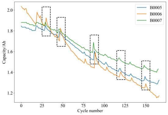
Figure 1.
NASA battery capacity degradation curves, with the rectangular boxes indicating notable points of capacity regeneration.
2.2. Extraction of Indirect Health Indicators
In the continuous charge and discharge cycles of lithium-ion batteries, ongoing electrochemical reactions occur internally, leading to a gradual deterioration in battery performance. Due to the highly complex electrochemical reaction mechanisms within the battery, the direct measurement of parameters such as internal resistance and capacity proves to be quite challenging. In contrast, parameters such as charge–discharge voltage, current, temperature, and time are relatively easy to obtain in practical application scenarios. Therefore, this paper proposes to start with indirect parameters considering real-world application scenarios.
To accurately predict the RUL of the battery, it is essential to select appropriate HI that reflect the aging condition of the battery. The operational state of the battery can be divided into two stages: charging and discharging. Due to significant variations during the discharging stage, extracting stable input features becomes challenging. Therefore, the HI are proposed to be extracted from the charging stage. In this study, the NASA lithium-ion battery cycling dataset is employed, and all cycles follow the same standard constant current-constant voltage charging protocol. Taking the B0005 battery as an example, the voltage and current variation curves under different charge–discharge cycles are illustrated in Figure 2.
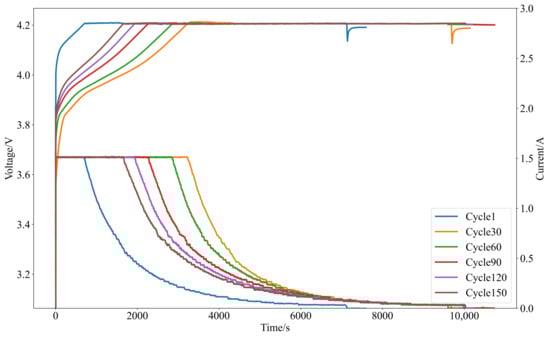
Figure 2.
Illustrates the voltage and current variation curves under different charge–discharge cycles.
Analysis reveals that the constant current charging time continues to increase, and the charging voltage exhibits a declining trend. Correspondingly, the constant voltage charging time shortens, and the charging current shows a decreasing trend. With the increase in the number of battery charge–discharge cycles, the degree of battery aging deepens continuously. It is concluded that the changes in voltage and current demonstrate good consistency with the battery aging process. In this study, three features are extracted as HI during the charging stage. HI1 represents the constant current charging time; HI2 represents the current variation during constant voltage charging for 1000 s; and HI3 represents the voltage variation during the first 500 s of charging.
From Figure 2, it is evident that the extracted HI do not follow a consistent pattern with the aging of the battery, making it difficult to directly assess their correlation with capacity. To further analyze the correlation between the three extracted HI and the original battery capacity from the dataset, this paper employs the Spearman correlation coefficient for a more quantitative analysis of each of the HI. When two variables exhibit a strong linear correlation, their correlation coefficient tends to approach either 1 or −1. A Spearman correlation coefficient of 1 indicates a perfect positive monotonic relationship, where both parameters consistently increase in tandem. Conversely, a correlation coefficient of −1 signifies a fully opposed or perfect consistent negative monotonic relationship between the two parameters, where one parameter consistently increases while the other decreases. On the contrary, if the two variables are independent of each other, the correlation coefficient is 0, indicating no monotonic relationship between the parameters as calculated by the formula:
where n is the length of the sequence, and and represent the mean values of x and y, respectively.
Table 1 presents the Spearman correlation coefficient results for the relationship between each of the HI and the battery capacity across three different batteries. It is evident that the Spearman correlation coefficients between each of the HI and battery capacity are close to 1 or −1, indicating a high correlation between the extracted battery HI and battery capacity.

Table 1.
Spearman correlation coefficients between battery HI and capacity.
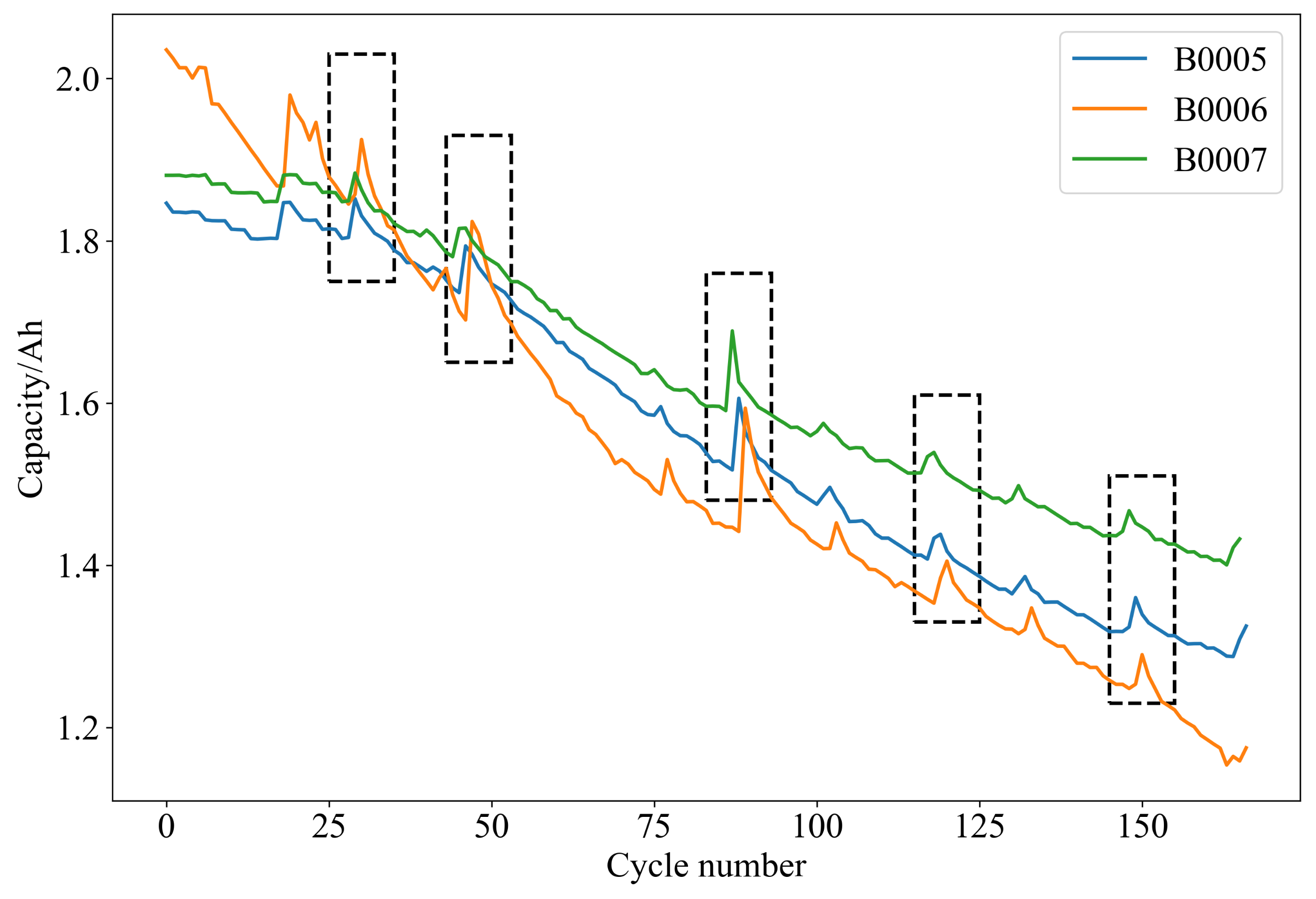
Figure 3 depicts the overall trends of the three extracted HI. It is observed that the overall trend of HI1 closely aligns with the degradation trend of battery capacity. The curve for HI2 exhibits rapid overall fluctuations, with noticeable peaks corresponding to the capacity rejuvenation points in the battery capacity degradation curve. In contrast, the curve for HI3 shows an opposite direction compared to the battery capacity degradation trend, and both exhibit minor fluctuations around the capacity regeneration points.
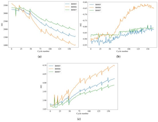
Figure 3.
The overall trend of HI. (a) HI1. (b) HI2. (c) HI3.
3. Methodology
3.1. Framework for RUL Prediction Based on CEEMDAN and CNN-BiGRU
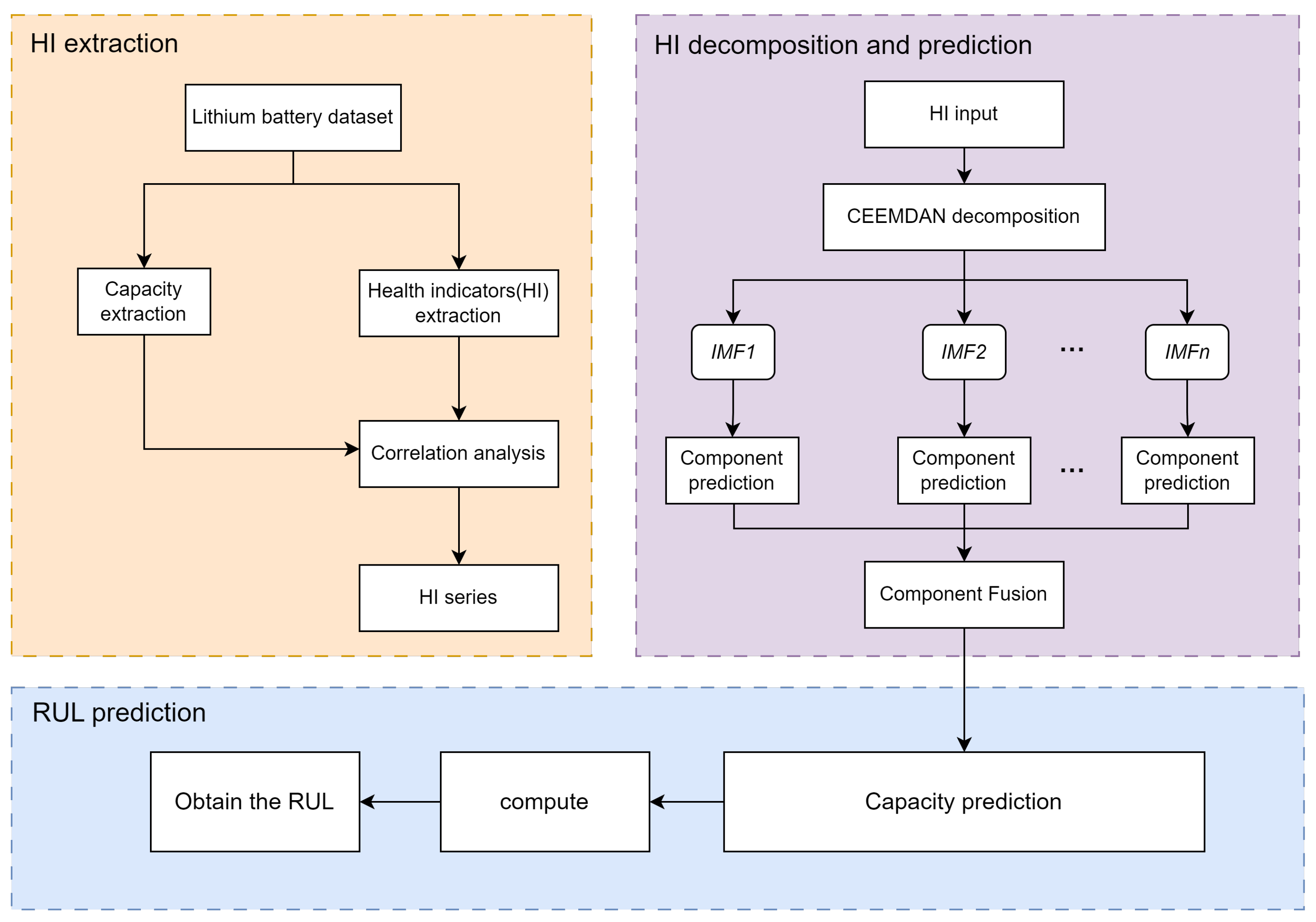
The RUL prediction method for lithium-ion batteries based on CEEMDAN and CNN-BiGRU proposed in this paper mainly consists of four stages. The algorithm framework is illustrated in Figure 4.
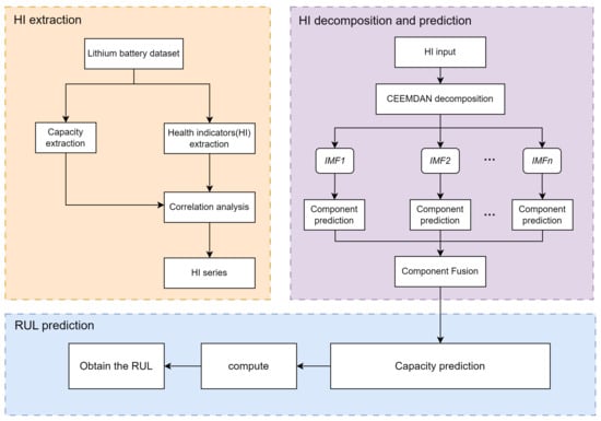
Figure 4.
Algorithm framework diagram.
- By analyzing the variation characteristics of current and voltage during the battery-charging phase and using correlation analysis to extract indirectly HI that highly reflect battery capacity decay, we optimize the input for battery RUL prediction.
- Utilizing the CEEMDAN algorithm to decompose HI, each decomposition results in several modal components and a residual component, reflecting the overall trend. Decomposing HI can decouple the trend component of overall change and the oscillation component of capacity regeneration, effectively suppressing regeneration phenomena in the sequence, and improving prediction accuracy.
- Establishing a CNN-BiGRU component prediction model. The decomposed components are divided into training and testing sets using the prediction starting point (ST). The CNN-BiGRU component prediction model is trained using the training set data, resulting in the component prediction model. Subsequently, the testing set data are input into the model for prediction, yielding the component prediction results.
- Establishing a CNN-BiGRU capacity prediction model. Using the extracted HI as multi-dimensional feature input and the corresponding battery capacity as a single-dimensional feature output, all HI and battery capacity data are divided into training and testing sets based on the ST. The capacity prediction model is trained, and finally, the component prediction results from the previous step are integrated to obtain HI as input. The model output is the predicted lithium-ion battery capacity, and the battery RUL prediction result can be calculated based on the set failure threshold.
3.2. CEEMDAN Decomposition of the HI Sequence
CEEMDAN is an adaptive signal processing method proposed by Torres et al. [20]. It is an improved algorithm based on EMD [21] and EEMD [22]. The EMD algorithm performs well in the decomposition of time series and exhibits strong adaptability to structurally complex data. However, it suffers from mode-mixing issues. The EEMD algorithm introduces white noise into the original sequence to address mode-mixing problems, but removing such white noise can be challenging. CEEMDAN incorporates the IMF components decomposed by the EMD algorithm back into the original sequence instead of directly introducing white noise. Additionally, the CEEMDAN algorithm calculates the average of each decomposition of the IMF components, addressing the issue of white noise being easily propagated and challenging to remove. In this paper, the CEEMDAN algorithm is employed to decompose the HI sequence, decoupling the trend component of overall change from the oscillation component of capacity regeneration. This enhances the subsequent prediction accuracy. The specific steps of the CEEMDAN decomposition are as follows:
In Step 1, adding white noise sequence to the HI sequence Z(t) is represented as follows:
where (t) represents the HI sequence after the i-th addition of white noise, a is the signal-to-noise ratio, and is a white noise sequence following a normal distribution.
In Step 2, the EMD algorithm is employed to decompose the signal Z(t) n times. The mean of the decomposition yields the first mode component, (t) as shown in Equation (3). Subsequently, Z(t) is subtracted by (t) to obtain the first residual signal (t) as expressed in Equation (4):
In Step 3, the first residual signal (t) is augmented with white noise to form a new sequence. This new sequence undergoes n rounds of EMD decomposition. The mean of the decomposition yields the second mode component (t) as shown in Equation (5). Subsequently, (t) is subtracted by (t) to obtain the second residual signal (t) as expressed in Equation (6):
Here, () represents the k-th mode component generated through EMD decomposition.
In Step 4, for each subsequent stage where k = 3,4,…,K, the solution method is analogous to Step 3. This process yields the k + 1-th mode component and the k + 1-th residual signal .
In Step 5, Step 4 is repeated until the obtained residual signal can no longer be further decomposed, leading to the cessation of the decomposition operation. Ultimately, the HI sequence Z(t) is decomposed into K mode components and a residual sequence R(t) as expressed in Equation (7):
3.3. CNN-BiGRU Prediction Model
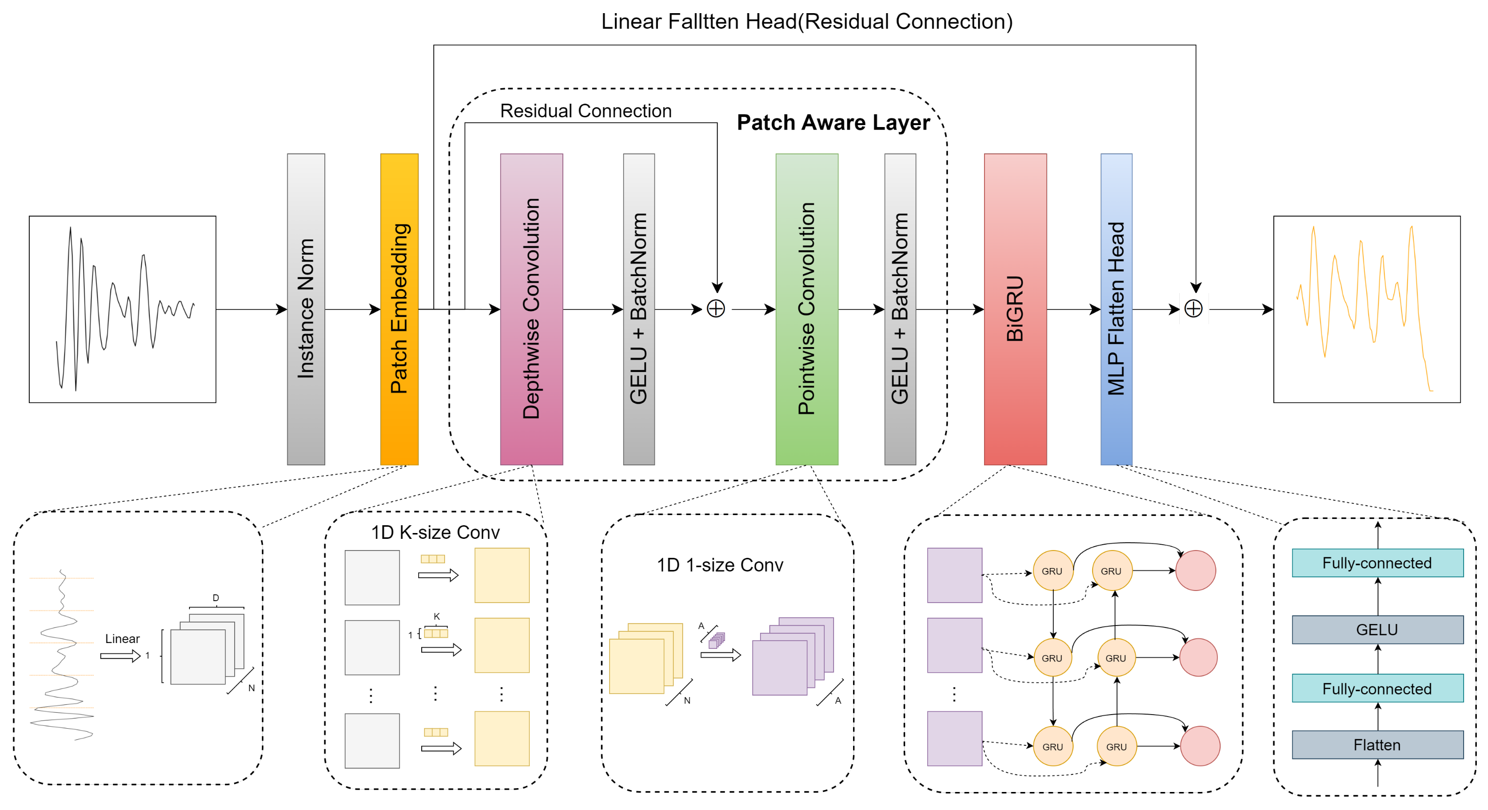
The overall architecture of the CNN-BiGRU prediction model is illustrated in Figure 5. In this paper, a CNN is employed to construct a Patch-Aware Layer for time series modeling. This design effectively utilizes the CNN to extract both global and local features of the time series data. Additionally, a BiGRU network is introduced to capture long-term dependencies within the time series. The paper also incorporates dual prediction heads, comprising a linear flatten head and an MLP flatten head. These prediction heads independently model future sequences by combining nonlinear and linear features. Subsequently, the predictions from the dual heads are merged to generate the final prediction. The following sections will provide detailed explanations of these components.
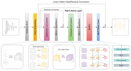
Figure 5.
Architecture diagram of the prediction model based on CNN-BiGRU.
3.3.1. Patch Embedding
Patch-based representations break down sequential time series data into smaller and structured segments, resembling image patches. This representation method extends single-dimensional time series data to two dimensions, aligning them with the characteristics of image data. This alignment enables the utilization of convolutional operations to capture both local and global features within the time series [23]. Patch embedding transforms the original one-dimensional univariate time series into a two-dimensional data structure similar to an image. Specifically, this paper employs the sliding window method to implement Patch embedding. This approach unfolds the input univariate time series through a sliding window of length P = 16 and a step size S = 8 as illustrated in the processing steps outlined in Equation (8):
3.3.2. Patch-Aware Layer
After processing through Patch embedding to obtain a two-dimensional sequence of image blocks, this paper utilizes a CNN to construct a Patch-Aware Layer for feature extraction and the modeling of the patch sequence. This module employs a single-scale depthwise separable convolution as the core component, using two convolutional approaches to extract both local and global information from the sequence. For the local information component, depthwise convolution is applied within each patch, facilitating local modeling in the patch dimension. For the global information component, a cross-patch pointwise convolution is used to model relationships between patches, enabling the model to capture both global and local features within the input sequence.
Depthwise convolution: This paper employs a specialized form of group convolution, where the number of groups is equal to the number of patches, denoted as N. To enlarge the receptive field, we use a larger kernel size, typically equal to the default step size S, i.e., K = 8. In this process, each input patch is convolved independently with a kernel, generating N feature maps, each corresponding to a specific patch. These feature maps are then sequentially concatenated to obtain the final feature mapping. Depthwise convolution effectively utilizes grouped convolution kernels, allowing the model to capture potential periodic patterns within each patch. Equation (9) below illustrates the process of a univariate series through the depthwise convolution kernel in layer l−1 to produce feature maps in layer l:
Pointwise convolution: Using only depthwise convolution may not effectively capture feature correlations between patches, so this paper incorporates pointwise convolution operations to enable information interaction between patches. Equation (11) illustrates the process of a variable sequence through the pointwise convolution kernel, where A represents the number of output channels in the pointwise convolution. After each convolution operation, we apply an activation function and post-activation BatchNorm, with denoting the GELU nonlinear activation function [24]. Additionally, we introduce a residual connection operation to avoid the problem of vanishing gradients and enhance network performance as shown in Equation (10):
3.3.3. BiGRU
Using only the Patch-Aware Layer constructed by CNN for feature extraction may overlook long-term dependencies between patches in the time series. Therefore, we introduce BiGRU. BiGRU is a type of Recurrent Neural Network (RNN) capable of capturing long-distance dependencies in sequences. The “bidirectional” aspect of the BiGRU model implies that, when processing sequence data, the model can consider information from both past and future time steps, enhancing its perception of dynamic changes in the time series. The model effectively handles long-term dependencies in sequences by controlling the flow of information through reset gates and update gates. Structurally, BiGRU can be viewed as a combination of forward and backward-propagating GRU. The hidden layer output (ht) at time t is the linear combination of the forward- and backward-propagating hidden layer outputs ( and ) at that time. Equation (12) describes the process of how the feature sequence undergoes deep modeling through BiGRU:
3.3.4. Dual Forecasting Heads
In this section, this paper employs a dual prediction head mechanism that focuses on both linear and nonlinear features. This approach allows the model to more effectively capture complex fluctuations in the time series. Specifically, the model utilizes a linear layer and a Multi-Layer Perceptron (MLP) layer as prediction heads. The linear layer captures the overall trend through a linear residual connection, while the MLP prediction head with a nonlinear function fits subtle variations in the curve. Finally, the output results from both prediction heads are summed to obtain the final prediction. Compared to the previous single linear head, the dual-head design demonstrates superior performance in prediction [23].
4. Experiments and Analysis of Results
To validate the effectiveness of the proposed prediction method, this paper conducts simulation experiments based on the lithium-ion battery aging dataset provided by NASA. By comparing and analyzing the predictive performance of different models, the paper aims to examine the prediction advantages of the proposed method. Additionally, the experiments test the adaptability and robustness of the prediction method by setting different STs. Comparative analysis of the prediction results from different methods is performed to further validate the predictive performance of the proposed method.
4.1. Performance Evaluation
This paper selects the Mean Absolute Error (MAE) and root mean square error (RMSE) as the accuracy evaluation metrics for the RUL prediction model, represented by Equations (13) and (14), respectively:
Here, represents the predicted capacity value, and represents the actual capacity value.
In the subsequent experiments, ST denotes the prediction starting point, represents the actual value from the prediction starting point to the end-of-life cycle, and represents the predicted value from the prediction starting point to the end-of-life cycle. The absolute error between the predicted RUL value and the actual RUL value is calculated using the equation:
4.2. Predict the HI Components
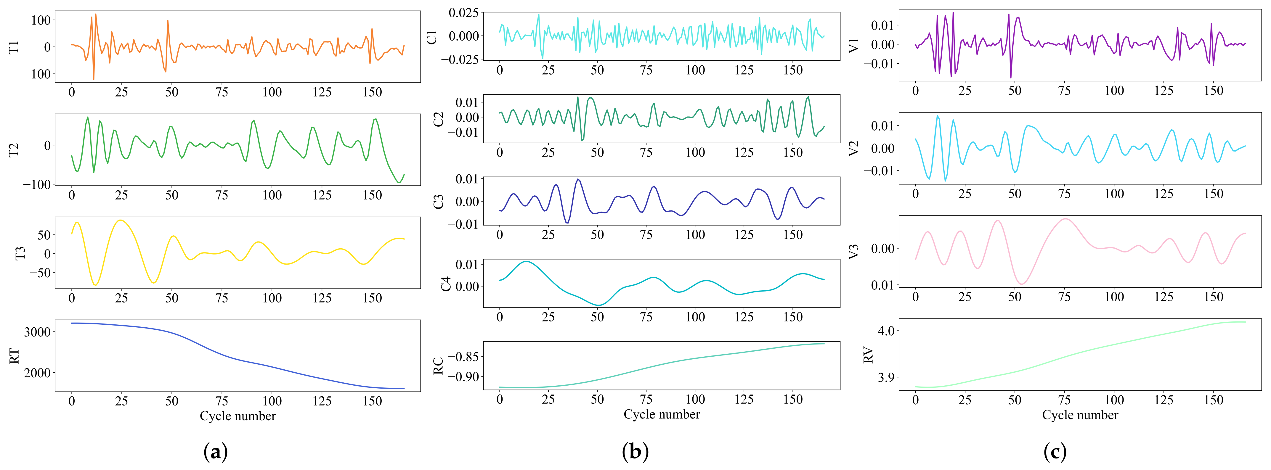
First, decompose the three HI values of each battery using CEEMDAN to obtain 13 components. Subsequently, input these 13 components into the component prediction model for forecasting.Taking battery B0005 as an example, HI1 is decomposed into T1, T2, T3, and RT; HI2 is decomposed into C1, C2, C3, C4, and RC; HI3 is decomposed into V1, V2, V3, and RV. Here, RT, RC, and RV represent residual components, while the others represent fluctuation components. The decomposition results are shown in Figure 6.
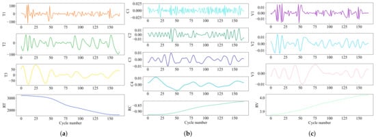
Figure 6.
CEEMDAN decomposition results of B0005 HIs. (a) HI1 decomposition results. (b) HI2 decomposition results. (c) HI3 decomposition results.
From Figure 6, it can be observed that each HI is decomposed into several fluctuation components and one residual component. The complexity of the fluctuation components gradually decreases with the increase in the series, and the residual component exhibits a monotonic decreasing or increasing trend. Analysis indicates that the fluctuation components collectively represent the local regeneration phenomena and fluctuations in the HI sequence, while the residual component captures the overall degradation trend with minor differences.
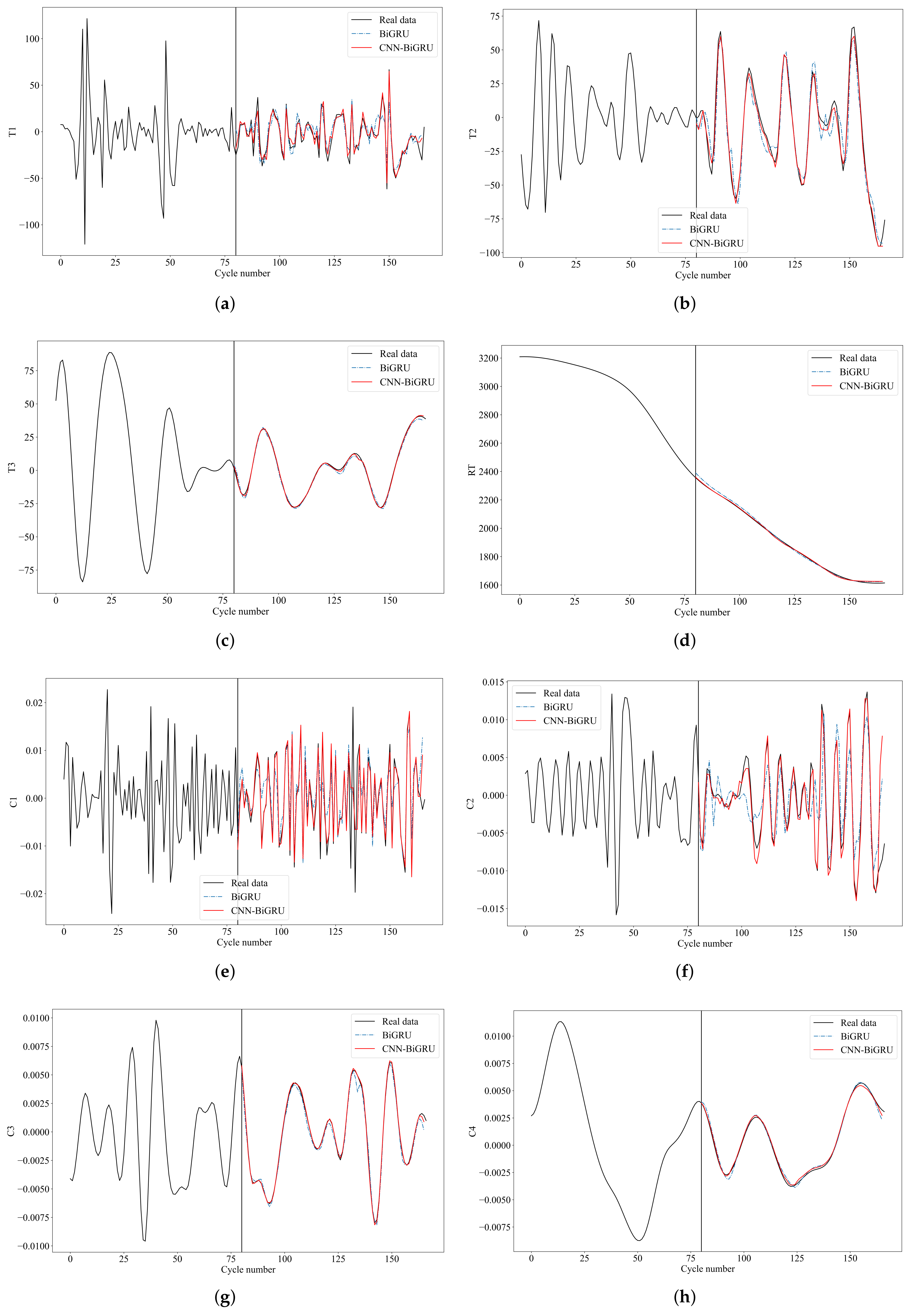
We conduct Spearman correlation coefficient analysis to assess the correlation between components and the original battery capacity. Table 2 reveals that the Spearman correlation coefficients for all residual components are close to 1 or −1, indicating a high correlation between residual components and the original battery capacity. This suggests that residual components can effectively characterize the overall degradation trend of the battery. The correlation between fluctuation components and the original capacity is relatively low. They reflect the local regeneration phenomena and fluctuations in the HI sequence. Accurate prediction of these components can reduce the impact of battery capacity regeneration on the prediction results, thereby enhancing the predictive performance of the capacity prediction model. Taking B0005 as an example, with a ST of 80, each component is input separately into the component prediction model. The component prediction models selected include BiGRU and CNN-BiGRU. The prediction results are shown in Figure 7.
Table 2.
Spearman correlation coefficient between component and capacity.
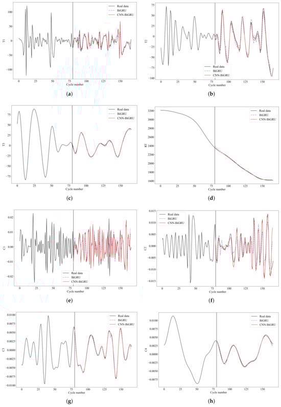
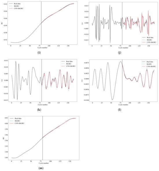
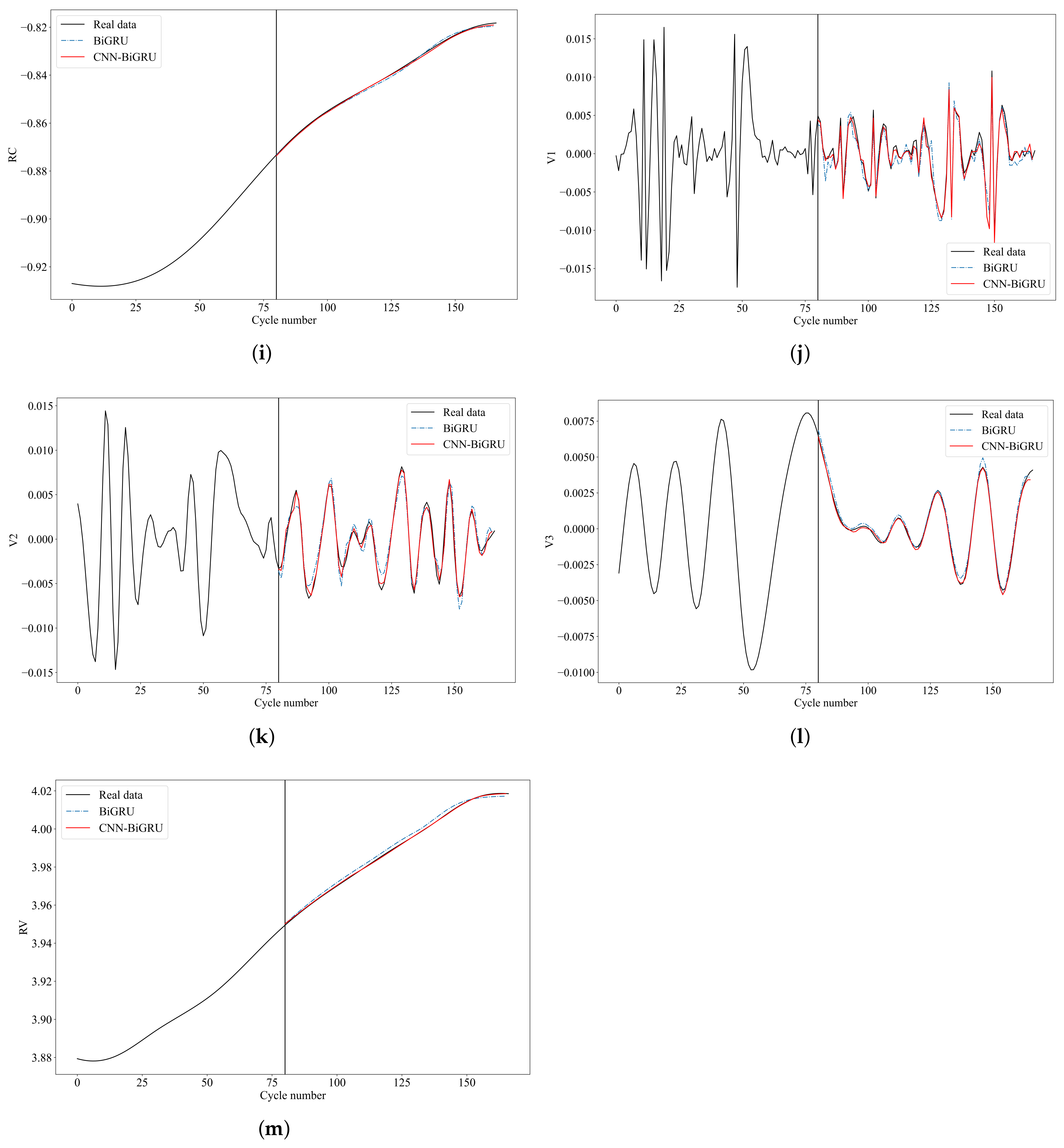
Figure 7.
Component prediction results. (a) T1. (b) T2. (c) T3. (d) RT. (e) C1. (f) C2. (g) C3. (h) C4. (i) RC. (j) V1. (k) V2. (l) V3. (m) RV.
From Figure 7, it can be observed that for components with strong fluctuation, the prediction performance after inputting them into the component prediction model is poor. This is due to inconsistent fluctuations before and after the component, resulting in relatively poor predictive performance, although the overall bias values are small. The trends of RT, RC, and RV components are more pronounced, leading to better prediction results. Moreover, when predicting components with strong fluctuations, CNN-BiGRU demonstrates better predictive performance compared to BiGRU.
4.3. Predict Battery RUL
Using ST, partition all HI and battery capacity data into training and testing sets. Train to obtain the capacity prediction model. Combine the component prediction results to form the original HI as the input and the corresponding battery capacity as output. Calculate the battery RUL prediction results based on the set failure threshold.
To validate the effectiveness of the proposed method, conduct comparative experiments between CEEDMAN-CNN-BiGRU, CEEDMAN-BiGRU, and CNN-BiGRU. Use the degradation dataset of batteries B0005, B0006, and B0007 for testing. Predictions are made with different starting points of 80 and 100. The RUL prediction results are presented in Table 3 and Figure 8.
Table 3.
RUL prediction results for different STs.
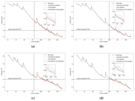
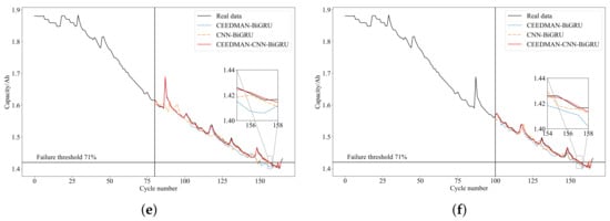
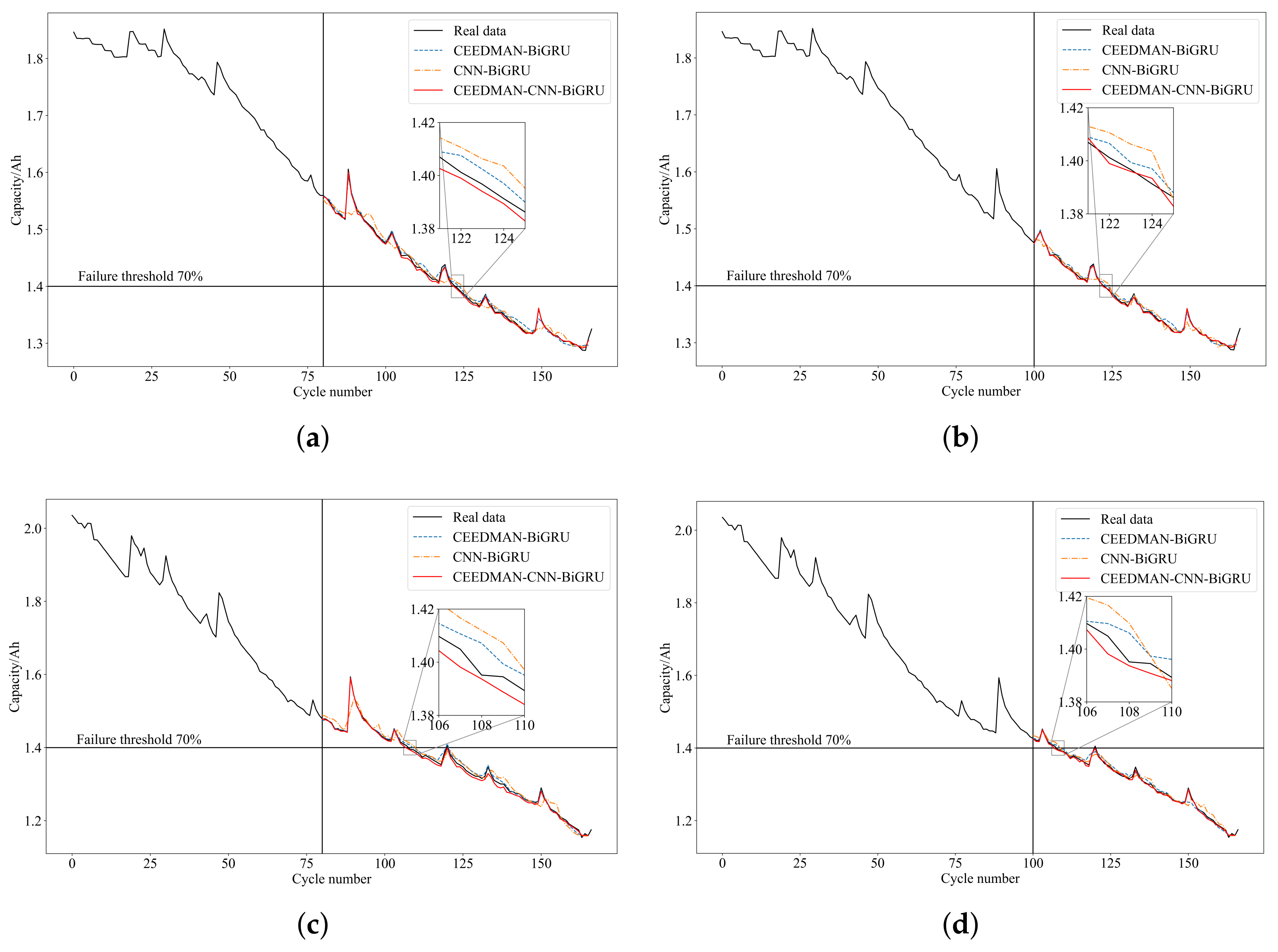
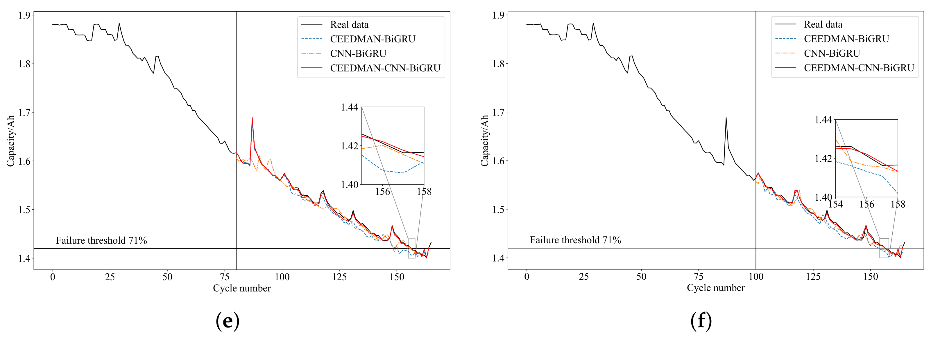
Figure 8.
Comparison of RUL prediction results at different STs. (a) B0005 (ST = 80). (b) B0005 (ST = 100). (c) B0006 (ST = 80). (d) B0006 (ST = 100). (e) B0007 (ST = 80). (f) B0007 (ST = 100).
From Table 3, it can be observed that when the ST is at 80 and 100, the proposed method in this paper provides more accurate RUL predictions compared to other methods. All evaluation metrics are optimal, and the prediction effectiveness varies for different batteries at different STs, with better performance as the ST increases. Figure 8 reveals that the prediction curve of the proposed method in this paper best fits the actual degradation curve, indicating the best prediction performance.
To further validate the effectiveness of this method, the proposed method is compared with recent RUL prediction methods such as SADE-MESN [25], UPF-LSSVM [26], BLS-RVM [16], IPSO-BPNN [27], PSO-RF [28], MHA-BiLSTM [29], TPE-CNN-BiGRU [30], MC-LSTM [31], and CEEMDAN-CNN-BiLSTM [32]. Predictions are made for different STs of 80 and 100, and the MAE and RMSE metrics are used to evaluate the prediction performance of each method. The specific comparison results are presented in Table 4.
Table 4.
Comparison of the RUL prediction results of the proposed method with the existing methods.
We have analyzed the above nine methods in detail. SADE-MESN utilizes a self-adaptive differential evolution algorithm to refine the parameters of a monotonic echo state network, thereby enhancing prediction accuracy. UPF-LSSVM merges data-driven and model-based algorithms, employing an unscented particle filter to track online battery capacity degradation and integrating it with the least squares support vector machine (LSSVM) for forecasting. BLS-RVM combines the broad learning system with the relevance vector machine, utilizing empirical mode decomposition for feature extraction, with the RVM acting as the predictive component. IPSO-BPNN leverages an improved particle swarm optimization algorithm alongside a backpropagation neural network to assess battery health and forecast RUL by optimizing the neural network’s initial weights and thresholds. PSO-RF uses a particle swarm optimization algorithm to determine the optimal parameters for a random forest, thereby enhancing the precision of RUL predictions. MC-LSTM introduces an innovative approach based on LSTM networks capable of handling multiple input channels, such as voltage, current, and temperature profiles, to improve generalization and mitigate the risk of battery failure. CEEMDAN-CNN-BiLSTM integrates CEEMDAN for data decomposition, a 1D CNN for feature extraction, and a BiLSTM network for precise RUL forecasting. TPE-CNN-BiGRU combines convolutional neural networks with bidirectional gated recurrent units and employs the Tree-structured Parzen Estimator (TPE) for adaptive hyperparameter optimization, bolstering the model’s stability and accuracy in RUL prediction. MHA-BiLSTM constructs a hybrid data preprocessing-based deep learning model that incorporates a multiscale hierarchical attention (MHA) mechanism within a BiLSTM network, effectively estimating RUL by considering the correlation and significance of each cycle’s information during the degradation process.
The various methods for predicting the RUL of lithium-ion batteries each have their own limitations. For example, SADE-MESN, UPF-LSSVM, and BLS-RVM primarily rely on smooth curve fitting, which introduces errors in predicting RUL, particularly when dealing with capacity regeneration phenomena. These methods do not accurately capture temporary performance rebounds of the battery and may lack the necessary sensitivity to rapid changes in battery degradation. IPSO-BPNN and PSO-RF, while improved in parameter optimization, may not effectively capture long-term dependencies in time-series data. MC-LSTM and TPE-CNN-BiGRU, which rely on indirect HI, do not account for the effects of capacity regeneration phenomena, potentially leading to suboptimal forecasting accuracy. CEEMDAN-CNN-BiLSTM uses capacity as direct HI but also fails to consider the implications of capacity regeneration. The MHA-BiLSTM multiscale hierarchical attention mechanism is adept at capturing the correlation and significance of each cycle’s information, but it may be computationally demanding and vulnerable to distortions caused by noisy data, thus potentially impacting the precision of its predictive capabilities.
In contrast, our proposed method stands out in predicting the RUL of lithium-ion batteries. Firstly, our method is particularly focused on capacity regeneration phenomena. This is a common phenomenon in the degradation process of lithium-ion batteries that significantly impacts prediction accuracy. By using the CEEMDAN method to decompose indirect HI into multiple scales, we can effectively separate the oscillatory components related to capacity regeneration, thereby reducing prediction errors. Secondly, our composite prediction model, which integrates CNN and BiGRU, not only extracts effective features from time-series data but also captures long-term dependency relationships, which is crucial for accurately predicting the remaining useful life of batteries. Lastly, our dual prediction head mechanism further enhances the model’s ability to handle linear and nonlinear features, making the predictions more precise and reliable.
From Table 4, it can be observed that under the same prediction starting point and dataset, compared with other methods, the proposed CEEDMAN-CNN-BiGRU method has a smaller MAE and RMSE, which means the error in RUL prediction is smaller and the method has higher precision, demonstrating better RUL prediction performance.
5. Conclusions
This paper proposes an indirect lithium-ion battery RUL prediction method based on CEEMDAN and CNN-BiGRU to overcome the limitations of existing methods in considering capacity regeneration phenomena. Firstly, by analyzing the current and voltage change characteristics during the battery-charging phase and combining correlation analysis, indirectly reflected HI that highly represent battery capacity decay are extracted, thereby optimizing the input for battery RUL prediction. Secondly, this paper applies the CEEMDAN method to perform the multiscale decomposition of HI, separating the overall trend and capacity regeneration oscillation into different components, effectively suppressing the impact of capacity regeneration phenomena on prediction accuracy. Subsequently, a composite prediction model integrating CNN and BiGRU is proposed. This model not only extracts global and local features of time series data effectively through Patch-Aware design but also significantly captures long-term dependency relationships in time series data using the BiGRU network. The introduction of a dual prediction head mechanism further enhances the model’s predictive capabilities in linear and nonlinear features. Finally, the method is validated using the lithium-ion battery dataset provided by NASA. Experimental results indicate that the proposed method can effectively capture capacity regeneration phenomena. It demonstrates stable performance when predicting from the starting points of 80 and 100, with a maximum average absolute error not exceeding 0.0096 and 0.0081, and a maximum root mean square error not exceeding 0.0196 and 0.0115. This method can effectively enhance the predictive accuracy of lithium-ion battery RUL, demonstrating its effectiveness and accuracy in predicting lithium-ion battery RUL.
This study not only suppresses capacity regeneration phenomena by optimizing input features but also introduces deep learning models to understand and model the capacity regeneration part, providing an innovative and effective method for lithium-ion battery RUL prediction. This method is of significant importance for improving the health monitoring and maintenance of battery systems, offering strong support for practical applications in battery management systems. Future research directions can focus on further improving the model structure, expanding applicable scenarios, and considering more real-world application factors.
Author Contributions
Methodology, K.L. and Z.M.; Validation, K.L.; Investigation, C.B. and G.L.; Resources, Z.M.; Data curation, K.L. and Z.M.; Writing—original draft, K.L., Z.M. and C.B.; Supervision, Z.M. All authors have read and agreed to the published version of the manuscript.
Funding
This work was supported by the National Natural Science Foundation of China (62166029) and the Inner Mongolia Autonomous Region Higher Education Carbon Peak and Carbon Neutrality Research Project (STZX202307).
Data Availability Statement
NASA Data Sources: https://www.nasa.gov/content/prognostics-center-of-excellence (accessed on 16 July 2022).
Conflicts of Interest
The authors declare no conflicts of interest.
Abbreviations
| Symbol | Definition |
| The value of the Spearman correlation coefficient | |
| The average value of variable x | |
| The average value of variable y | |
| Add white noise for the i-th time | |
| (t) | The HI sequence after the i-th addition of white noise |
| The signal-to-noise ratio | |
| (t) | The k-th modal component obtained by decomposition |
| The k-th mode component generated through EMD decomposition | |
| The k-th residual signal | |
| One-dimensional time series | |
| Two-dimensional time series | |
| The univariate series passing through the depthwise convolution kernel to generate feature maps in the l layer | |
| The univariate series passing through the pointwise convolution kernel to generate feature maps in the l-layer | |
| The hidden layer output at time t | |
| The forward-propagating hidden layer output at time t | |
| The backward-propagating hidden layer output at time t | |
| The weight of the forward-propagating GRU unit’s hidden layer output at time t | |
| The weight of the backward-propagating GRU unit’s hidden layer output at time t | |
| The corresponding bias term for | |
| The predicted capacity value at the i-th cycle | |
| The actual capacity value at the i-th cycle | |
| The absolute error between the predicted RUL value and the actual RUL value | |
| The predicted RUL value | |
| The actual RUL value |
References
- Sarmah, S.B.; Kalita, P.; Garg, A.; Niu, X.D.; Zhang, X.W.; Peng, X.; Bhattacharjee, D. A review of state of health estimation of energy storage systems: Challenges and possible solutions for futuristic applications of li-ion battery packs in electric vehicles. J. Electrochem. Energy Convers. Storage 2019, 16, 040801. [Google Scholar] [CrossRef]
- Tian, H.; Qin, P.; Li, K.; Zhao, Z. A review of the state of health for lithium-ion batteries: Research status and suggestions. J. Clean. Prod. 2020, 261, 120813. [Google Scholar] [CrossRef]
- Lipu, M.H.; Hannan, M.; Hussain, A.; Hoque, M.; Ker, P.J.; Saad, M.H.M.; Ayob, A. A review of state of health and remaining useful life estimation methods for lithium-ion battery in electric vehicles: Challenges and recommendations. J. Clean. Prod. 2018, 205, 115–133. [Google Scholar] [CrossRef]
- Zhu, J.; Tan, T.; Wu, L.; Yuan, H. RUL prediction of lithium-ion battery based on improved DGWO-ELM method in a random discharge rates environment. IEEE Access 2019, 7, 125176–125187. [Google Scholar] [CrossRef]
- Lin, C.P.; Cabrera, J.; Yang, F.; Ling, M.H.; Tsui, K.L.; Bae, S.J. Battery state of health modeling and remaining useful life prediction through time series model. Appl. Energy 2020, 275, 115338. [Google Scholar] [CrossRef]
- Pang, X.; Huang, R.; Wen, J.; Shi, Y.; Jia, J.; Zeng, J. A lithium-ion battery RUL prediction method considering the capacity regeneration phenomenon. Energies 2019, 12, 2247. [Google Scholar] [CrossRef]
- Liu, Q.; Zhang, J.; Li, K.; Lv, C. The remaining useful life prediction by using electrochemical model in the particle filter framework for lithium-ion batteries. IEEE Access 2020, 8, 126661–126670. [Google Scholar] [CrossRef]
- Guha, A.; Patra, A. State of health estimation of lithium-ion batteries using capacity fade and internal resistance growth models. IEEE Trans. Transp. Electrif. 2017, 4, 135–146. [Google Scholar] [CrossRef]
- Peng, Y.; Hou, Y.; Song, Y.; Pang, J.; Liu, D. Lithium-ion battery prognostics with hybrid Gaussian process function regression. Energies 2018, 11, 1420. [Google Scholar] [CrossRef]
- Yao, F.; He, W.; Wu, Y.; Ding, F.; Meng, D. Remaining useful life prediction of lithium-ion batteries using a hybrid model. Energy 2022, 248, 123622. [Google Scholar] [CrossRef]
- Yu, Y.; Hu, C.; Si, X.; Zheng, J.; Zhang, J. Averaged Bi-LSTM networks for RUL prognostics with non-life-cycle labeled dataset. Neurocomputing 2020, 402, 134–147. [Google Scholar] [CrossRef]
- Zhao, L.; Wang, Y.; Cheng, J. A hybrid method for remaining useful life estimation of lithium-ion battery with regeneration phenomena. Appl. Sci. 2019, 9, 1890. [Google Scholar] [CrossRef]
- Zhang, J.; Jiang, Y.; Li, X.; Luo, H.; Yin, S.; Kaynak, O. Remaining useful life prediction of lithium-ion battery with adaptive noise estimation and capacity regeneration detection. IEEE/ASME Trans. Mechatronics 2022, 28, 632–643. [Google Scholar] [CrossRef]
- Wang, Y.; Pan, R.; Yang, D.; Tang, X.; Chen, Z. Remaining useful life prediction of lithium-ion battery based on discrete wavelet transform. Energy Procedia 2017, 105, 2053–2058. [Google Scholar] [CrossRef]
- Li, X.; Zhang, L.; Wang, Z.; Dong, P. Remaining useful life prediction for lithium-ion batteries based on a hybrid model combining the long short-term memory and Elman neural networks. J. Energy Storage 2019, 21, 510–518. [Google Scholar] [CrossRef]
- Chen, Z.; Shi, N.; Ji, Y.; Niu, M.; Wang, Y. Lithium-ion batteries remaining useful life prediction based on BLS-RVM. Energy 2021, 234, 121269. [Google Scholar] [CrossRef]
- Yang, Z.; Wang, Y.; Kong, C. Remaining useful life prediction of lithium-ion batteries based on a mixture of ensemble empirical mode decomposition and GWO-SVR model. IEEE Trans. Instrum. Meas. 2021, 70, 2517011. [Google Scholar] [CrossRef]
- Lyu, G.; Zhang, H.; Zhang, Y.; Miao, Q. An interpretable remaining useful life prediction scheme of lithium-ion battery considering capacity regeneration. Microelectron. Reliab. 2022, 138, 114625. [Google Scholar] [CrossRef]
- Saha, B.; Goebel, K. Battery data set. In NASA AMES Prognostics Data Repository; NASA Ames Research Center: Moffett Field, CA, USA, 2007. [Google Scholar]
- Torres, M.E.; Colominas, M.A.; Schlotthauer, G.; Flandrin, P. A complete ensemble empirical mode decomposition with adaptive noise. In Proceedings of the 2011 IEEE International Conference on Acoustics, Speech and Signal Processing (ICASSP), Prague, Czech Republic, 22–27 May 2011; pp. 4144–4147. [Google Scholar]
- Huang, N.E.; Shen, Z.; Long, S.R.; Wu, M.C.; Shih, H.H.; Zheng, Q.; Yen, N.C.; Tung, C.C.; Liu, H.H. The empirical mode decomposition and the Hilbert spectrum for nonlinear and non-stationary time series analysis. Proc. R. Soc. Lond. Ser. A Math. Phys. Eng. Sci. 1998, 454, 903–995. [Google Scholar] [CrossRef]
- Wu, Z.; Huang, N.E. Ensemble empirical mode decomposition: A noise-assisted data analysis method. Adv. Adapt. Data Anal. 2009, 1, 1–41. [Google Scholar] [CrossRef]
- Gong, Z.; Tang, Y.; Liang, J. PatchMixer: A Patch-Mixing Architecture for Long-Term Time Series Forecasting. arXiv 2023, arXiv:2310.00655. [Google Scholar]
- Hendrycks, D.; Gimpel, K. Gaussian error linear units (gelus). arXiv 2016, arXiv:1606.08415. [Google Scholar]
- Ji, Y.; Chen, Z.; Shen, Y.; Yang, K.; Wang, Y.; Cui, J. An RUL prediction approach for lithium-ion battery based on SADE-MESN. Appl. Soft Comput. 2021, 104, 107195. [Google Scholar] [CrossRef]
- Li, X.; Ma, Y.; Zhu, J. An online dual filters RUL prediction method of lithium-ion battery based on unscented particle filter and least squares support vector machine. Measurement 2021, 184, 109935. [Google Scholar] [CrossRef]
- Ma, Y.; Yao, M.; Liu, H.; Tang, Z. State of health estimation and remaining useful life prediction for lithium-ion batteries by improved particle swarm optimization-back propagation neural network. J. Energy Storage 2022, 52, 104750. [Google Scholar] [CrossRef]
- Wu, J.; Cheng, X.; Huang, H.; Fang, C.; Zhang, L.; Zhao, X.; Zhang, L.; Xing, J. Remaining useful life prediction of Lithium-ion batteries based on PSO-RF algorithm. Front. Energy Res. 2023, 10, 937035. [Google Scholar] [CrossRef]
- Luo, T.; Liu, M.; Shi, P.; Duan, G.; Cao, X. A Hybrid Data Preprocessing-Based Hierarchical Attention BiLSTM Network for Remaining Useful Life Prediction of Spacecraft Lithium-Ion Batteries. IEEE Trans. Neural Netw. Learn. Syst. 2023. [Google Scholar] [CrossRef] [PubMed]
- Zheng, X.; Chen, D.; Wang, Y.; Zhuang, L. Remaining useful life indirect prediction of lithium-ion batteries using CNN-BiGRU fusion model and TPE optimization. AIMS Energy 2023, 11, 896–917. [Google Scholar] [CrossRef]
- Park, K.; Choi, Y.; Choi, W.J.; Ryu, H.Y.; Kim, H. LSTM-based battery remaining useful life prediction with multi-channel charging profiles. IEEE Access 2020, 8, 20786–20798. [Google Scholar] [CrossRef]
- Guo, X.; Wang, K.; Yao, S.; Fu, G.; Ning, Y. RUL prediction of lithium ion battery based on CEEMDAN-CNN BiLSTM model. Energy Rep. 2023, 9, 1299–1306. [Google Scholar] [CrossRef]

Disclaimer/Publisher’s Note: The statements, opinions and data contained in all publications are solely those of the individual author(s) and contributor(s) and not of MDPI and/or the editor(s). MDPI and/or the editor(s) disclaim responsibility for any injury to people or property resulting from any ideas, methods, instructions or products referred to in the content. |
© 2024 by the authors. Licensee MDPI, Basel, Switzerland. This article is an open access article distributed under the terms and conditions of the Creative Commons Attribution (CC BY) license (https://creativecommons.org/licenses/by/4.0/).