School Electricity Consumption in a Small Island Country: The Case of Fiji

Abstract

Electricity consumption in buildings is one of the major causes of energy usage and knowledge of this can help building owners and users increase energy efficiency and conservation efforts. For Pacific Island countries, building electricity demand data is not readily accessible or available for constructing models to predict electricity demand. This paper starts to fill this gap by studying the case of schools in Fiji. The aim of the paper is to assess the factors affecting electricity demand for grid-connected Fijian schools and use this assessment to build mathematical models (multiple linear regression (MLR) and artificial neural network (ANN)) to predict electricity consumption. The average grid-connected electricity demand in kWh/year was 1411 for early childhood education schools, 5403 for primary schools, and 23,895 for secondary schools. For predicting electricity demand (ED) for all grid-connected schools, the stepwise MLR model shows that taking logarithm transformations on both the dependent variable and independent variables (number of students, lights, and air conditioning systems) yields statistically significant independent variables with an R² value of 73.3% and RMSE of 0.2248. To improve the predicting performance, ANN models were constructed on both the natural form of variables and transformed variables. The optimum ANN model had an R² value of 95.3% and an RMSE of 59.4 kWh/year. The findings of this study can assist schools in putting measures in place to reduce their electricity demand, associated costs, and carbon footprint, as well as help government ministries make better-informed policies.

1. Introduction

Climate change is an existential threat to planet Earth, and countries, individually and collectively, are putting various measures in place to combat and adapt to it. One such measure is demand-side energy management, which requires knowledge of building energy use. Such knowledge can help benchmark the energy demand of buildings [1] which leads to growth in energy efficiency and conservation efforts and informs policy makers [2]. As a result, these actions can reduce greenhouse gas (GHG) emissions from buildings [3]. According to Guo [4], the building industry is anticipated to be crucial in the energy transition, reducing climate change globally, and achieving sustainable development goals. Hence, as a first case, this study focuses on assessing school electricity consumption and predicting electricity demand to understand the factors that influence the usage.

Energy management for schools is much needed as, apart from the above-mentioned reasons, it will also encourage behavioral change in the younger generation to conserve energy and use it efficiently. Earlier studies related to energy consumption in schools have focused on the statistical analysis of secondary data and these studies are based in countries that are not in the Pacific region, such as European countries, the United States of America, Japan, Hong Kong, Malaysia, South Korea, and others [5]. Primary energy use data in schools and day care centers in southern Finland studied by Airaksinen [6] showed that when special attention is paid during design and construction phase of buildings, it promotes energy efficiency. High schools in Hong Kong were studied using a two-stage regression-based approach that informed researchers of crucial factors that influence the energy utilization index of schools [7]. Senior and junior high schools and elementary schools in Taiwan were studied by Wang [8] and they found that air conditioning and lighting heavily influenced the electricity consumption of schools. These studies also report that energy consumption in schools is dominated by electricity for lights and cooling and gas for space heating.

Chung and Yeung [7] studied the energy performance of secondary schools in Hong Kong and they comprehensively discussed the energy utilization index (EUI) of various schools based either on the electricity consumed or heating energy requirements in different countries. Chung and Yeung [9] found that the average energy consumption and energy use intensity per school are 530 MWh and 105.61 kWh/m²/year, respectively. Canadian schools’ median total energy consumption (257 kWh/m²/year) was 29% higher than other Canadian benchmarks (200 kWh/m²/year) and the school building age had a statistically significant effect on their energy consumption, with newer schools consuming less gas but more electricity than older and middle-aged ones [10]. Energy consumption in Europe varies from 10 to 30 kWh/m² annually [11].

Further, the cumulative sum (CUSUM) method was used by Stuart et al. [12] to study half-hourly electricity data for a secondary school in the UK to identify shifts in electricity consumption patterns for buildings while Samuels and Booysen [13] used controlled human behavioral experiments in South African schools to reduce electricity consumption, its costs, and dependence on fossil fuels. Similarly, to save electricity, school children can participate in energy-saving contests, nudging family members to save electricity in their homes [14]. Therefore, students can be seen as agents of behavioral change that can aid in energy saving not only in schools but at homes as well. Apart from behavioral changes, schools can also employ energy audits to provide insights into how the energy-specific usage index could be an essential tool for explaining the electricity consumption of schools and thus lead to energy saving [15]. A detailed energy audit framework was proposed by Corrado et al. [16] using school buildings in Italy and technical and financial solutions were proposed as part of its audit. A simpler lighting energy audit was carried out by Shailesh et al. [17] for classrooms in an academic institute and recommended using energy-efficient technologies and controls to improve lighting and efficiency.

Knowledge of the current electricity demand of a school building can also help create models for predicting electricity demand and assessing factors that most affect electricity demand, which leads to the benchmarking of building energy use similar to the work performed by Borgstein and Lamberts [18] for bank buildings. Recently, a top-down energy benchmarking methodology based on the actual energy consumption within a cluster of governmental office buildings was used by Vaisi et al. [19] and provides reference points for measuring and rewarding buildings with good performance while buildings with poor performance can be prioritized for improvement. Machine learning can also be used to develop energy benchmarking and efficiency scales in buildings [20]. School building energy consumption is dependent on the floor area, number of floors, number of classrooms, number of window-type air conditioners, light system, percentage of lighting control [7], number of classes [21], location, total roof area, building age, number of students, and type of school [22]. Different techniques can be used for modeling and predicting building energy use, such as statistical regressions, autoregressive models, support vector machines (SVM), artificial neural networks (ANN), ensembled models, and combined models [23]. The energy audit data can be used to build linear regression models to predict energy or electricity demand for schools and determine how different factors affect electricity consumption or gas consumption in schools [15]. Researchers can also use secondary data sources from the relevant education departments [8] such as building, utility company, and national statistics to carry out regression analyses on electricity or gas consumption in buildings [24]. However, without doing a detailed energy audit, some researchers use targeted surveys to collect the necessary data for regression analyses. For instance, Almeida et al. [25] proposed a methodology for estimating the water and energy consumption in university buildings while Nematchoua et al. [26] designed a questionnaire to collect energy consumption data in different types of buildings (residential and commercial) in 12 cities in Madagascar. Furthermore, Ma et al. [27] collected energy consumption data from on-site surveys of 17 schools in Tianjin, China and found that a variety of energy sources such as electricity, natural gas, municipal heating, coal, gasoline, diesel oil, tap water, reclaimed water, and alcohol-based fuels were consumed by the 17 schools, while 15 states in Brazil joined a survey to provide necessary data from 5321 schools that were used to build a regression model for annual energy consumption [28].

Autoregressive models and statistical regression are popular conventional methods for building energy consumption monitoring and forecasting and provide a good balance between implementation simplicity and forecasting accuracy [23]. Wu et al. [29] adopted a linear regression model to determine the impact of different functional areas on the total energy consumption of multifunctional building types, while Chung and Yeung conducted a two-stage regression analysis [7]; first backward, forward, and stepwise (Ordinary Least Square) regression analyses and then, if a regression model with better goodness-of-fit was necessary, convex nonparametric least squares (CNLS) regression analyses were conducted. Using correlation analysis and multiple linear regression (MLR) analysis, it was found that the total energy consumption, energy utilization index, and energy usage per person were positively correlated with campus area, total floor area, and the number of students [8].

In addition, Mohammed et al. [22] concluded that their regression model demonstrated an accuracy of more than 95% after a comparison to data collected from actual school facilities in Saudi Arabia. To determine the effect of building age, school type, number of occupants, occupant density, and floor area on energy consumption, three multiple regression models were developed by Ouf and Issa [10]. These models aimed to determine how much of the variation in average annual electricity, gas, and total energy consumption in Manitoba’s school buildings was due to these factors.

However, for some datasets, MLR can be rigid; for example, it can only be used when a set of assumptions are met and when there is a linear relationship between independent variables and the dependent variable. In such cases, an artificial neural network (ANN) gives more flexibility in predicting electricity demand. The advantage of the ANN method is that it does not assume a linear relationship between dependent and independent variables; instead, it can model non-linear relationships by partitioning the data set into a training set and testing the model [30]. The hourly electricity consumption for a university campus in Japan was predicted using an ANN and the R² between the actual measurement and the ANN model’s prediction was found to range between 0.96 and 0.99 at the training stage, and between 0.95 and 0.99 at testing stage [31]. Similarly, Alshibani [32] used an ANN to predict the energy consumption of schools in Saudi Arabia. Researchers have also used different methods to compare model performance for predicting electricity consumption. For instance, Jeong et al. [30] used seasonal autoregressive integrated moving average (SARIMA) and an ANN to predict electricity consumption in three different schools using IBM Statistical Package for the Social Sciences (SPSS) 21.0 software while Nsangou et al. [33] used quantile regression and an ANN to understand the factors affecting household electricity consumption. Likewise, energy consumption prediction for office buildings was performed using three methods in SPSS (ANN, SVM (Support vector regression), and ARIMA) and the researchers recommended using ANN and SVM methods for energy consumption prediction [34]. In addition, Panklib [35] used MLR and an ANN to predict the annual electricity consumption in Thailand. These researchers used various parameters such as mean absolute error (MAE), mean absolute percentage error (MAPE), root mean square error (RSME), and coefficient of determination (R²) for assessing the performance of predictive models. On the other hand, Chen et al. [36] have predicted office building electricity demand using the ANN method by splitting the time horizons into two occupancy-based periods (no occupancy times and full occupancy times).

Building Energy Use in Fiji

In Fiji, around 40–50% of all electricity generated is from industrial diesel oil and heavy fuel oil, while the remaining is from hydropower, biomass, solar, and wind [37]. The most recent research in Fiji focuses on the supply side of energy, not the demand side. For instance, Joseph and Prasad [38] assessed the municipal solid waste for electricity generation in Fiji and the Pacific while Prasad and Raturi [39] studied various technologies for meeting the electricity demand in Fiji. The lack of energy consumption data for buildings in Fiji is highlighted in [40], which is one of the main reasons for the lack of research on building energy demand. Fiji’s National Adaptation Plan [41] identifies energy data collection as a priority while Fiji’s nationally determined contributions (NDCs) also target energy efficiency measures to reduce 10% of the business-as-usual greenhouse gas emissions by 2030 economy-wide, including electricity demand-side sub-sectors [42]. According to global studies, the usual energy sources consumed in schools are electricity for meeting cooling loads and other electrical loads and gas for meeting the space heating demand. For Fiji and other Pacific Island countries, it should be noted that schools do not need space heating due to their relatively close proximity to the equator; hence, electricity is the major form of energy consumption in schools.

The literature review reveals that energy consumption data of different sectors of the economy in Fiji is not the latest. Siwatibau [43] carried out an energy survey of selected households (1011 electrified and 301 unelectrified), 76 industrial companies, 77 commercial companies, and 10 large office buildings in Suva, the capital city of Fiji. However, it is noted that this research was performed almost 35 years ago, and schools were not included in this research. Another study conducted an energy survey assessment of rural households in Fiji in 2003 and focused attention on rural electrification [24] but did not study school energy usage. Prasad and Raturi [44] have used multiple linear regression (MLR) models to forecast Fiji’s electricity demand for non-domestic and domestic customers, where schools were not explicitly covered.

It is to be noted that electricity is one of the major costs for operating schools. According to 2020 statistics, there are 871 early childhood education (ECE) schools in Fiji, 736 primary schools and 171 secondary schools [45]. Like other small island nations, Fiji has some schools connected to the national electricity grid and some off-grid, meaning not connected to the national grid, and thus have distributed generation either from diesel generators or other renewable energy sources such as solar. For Fiji, it is hypothesized that the main form of energy consumption is electricity in schools (as seen from Siwatibau’s [43] research), with a negligible need for space heating energy. However, no studies assess electricity consumption for schools in Fiji or the factors that affect electricity consumption and models for predicting electricity demand. Even though electricity consumption in schools is small compared to the national electricity consumption, carrying out an electricity demand assessment study in schools and sharing the findings will help raise awareness of electricity monitoring, set benchmarks, predict electricity usage, and improve energy efficiency and conservation efforts.

According to the aforementioned literature engagement, studies do not exist for electricity prediction for island nations such as those in the Pacific where electricity is the major form of energy consumption of buildings with a minimal or negligible energy requirement for space heating. In addition, there are no studies that have successfully predicted the electricity consumption of educational facilities in Fiji. Hence, the primary aim of the current study is to gain a better understanding of factors affecting electricity demand for grid-connected Fijian schools and use it to build mathematical models to predict electricity consumption in schools using MLR and ANNs. The main research question of the study is: What factors affect electricity demand in Fijian schools and how do mathematical models such as MLR and ANN perform when predicting electricity demand? Hence, the specific objectives of this paper are as follows: (i) assess (identify, quantify, and report) electricity demand in different clusters of grid-connected schools around Fiji, (ii) construct MLR and ANN models for predicting electricity demand in grid-connected schools and determine the factors that most affect electricity consumption, and (iii) compare the performance of MLR and ANN methods for predicting electricity consumption. The novelty of this work is that it will add to the literature on electricity use in small developing island nations that do not require space heating in buildings. Also, it will contribute to the body of knowledge on schools’ electricity demand in Fiji and assist work on building energy performance assessment, planning, and policymaking. In addition, this study also compares conventional MLR and ANN prediction models and their performance using two performance indices: R² and RMSE.

The next section of the paper discusses the methodology used for the present work, followed by Section 3, which presents and discusses the questionnaire survey results. Section 3 also presents the descriptive statistics of the annual electricity demand for different clusters of schools and building characteristics. It further presents and discusses the results of the MLR and ANN models, and tests the performance of these models. Section 4 discusses the limitations and implications of the present work. Finally, in Section 5, some conclusions are made.

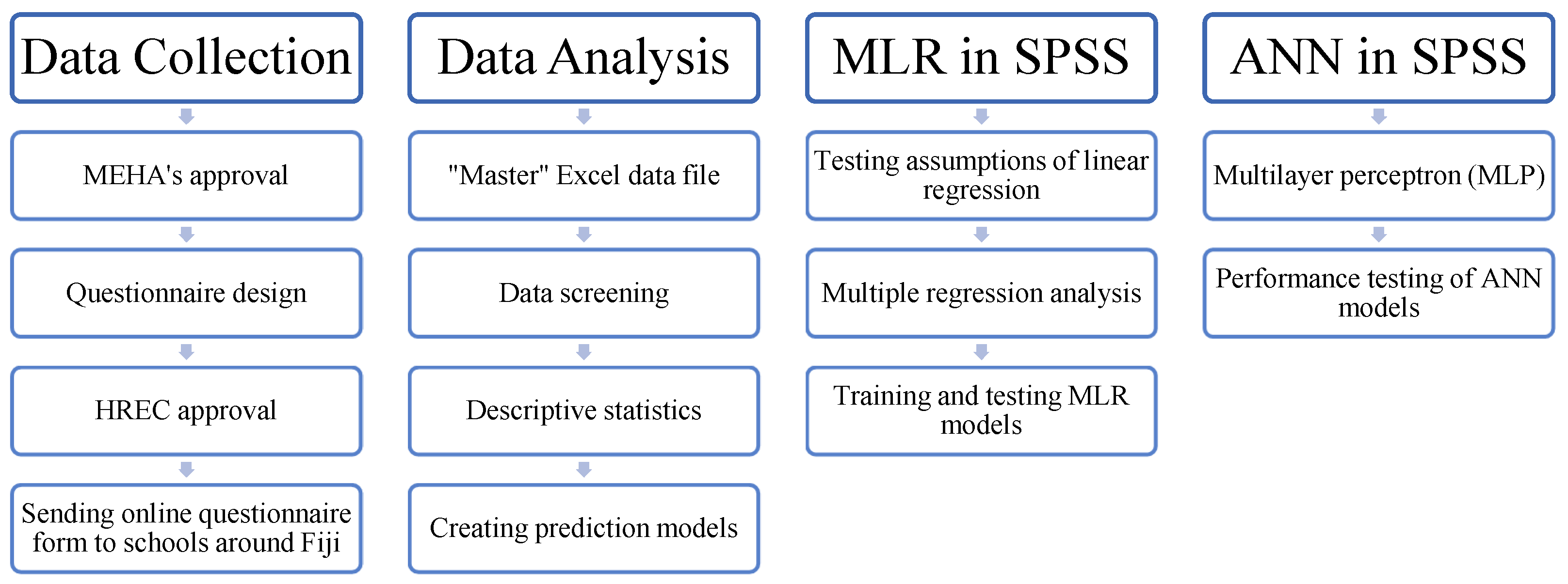
2. Materials and Methods

This research adopted a mixed method approach of both qualitative and quantitative methods. The Ministry of Education, Heritage, and Arts (MEHA) in Fiji was contacted to seek their approval in carrying out the research, which included making a written application to the Policy Unit of the Corporate Services division of the MEHA.

2.1. Questionnaire Design

A questionnaire survey was designed to collect data on the current green initiatives undertaken by the schools, their year of establishment, the number of students, teachers, and ancillary staff, building characteristics (such as total internal floor area, number of buildings, stories, types of building, and number of classrooms) similar to data collected by Rinaldi et al. [46], electricity use profile (annual electricity consumption data and its costs), number of different electrical appliances used in schools (air conditioners, computers, fans, lights, etc.), and information on any other energy source. Both open-ended and multiple-choice questions were used. The sample of questions can be found in Supplementary Data S1.

The principles provided by Groves et al. [47] were used to ensure that the survey was not biased. Questions were clear and followed a logical order, and ambiguous language was avoided. Human research ethics approval was also sought from the author’s university’s Human Research Ethics Committee (HREC), and participants were made aware of the voluntary nature of participation and ways in which data will be stored, analyzed, and disseminated. As this research was about energy data and building characteristics, it did not involve questions on a sensitive nature, such as culturally sensitive issues, or cause physical, psychological, or social discomfort.

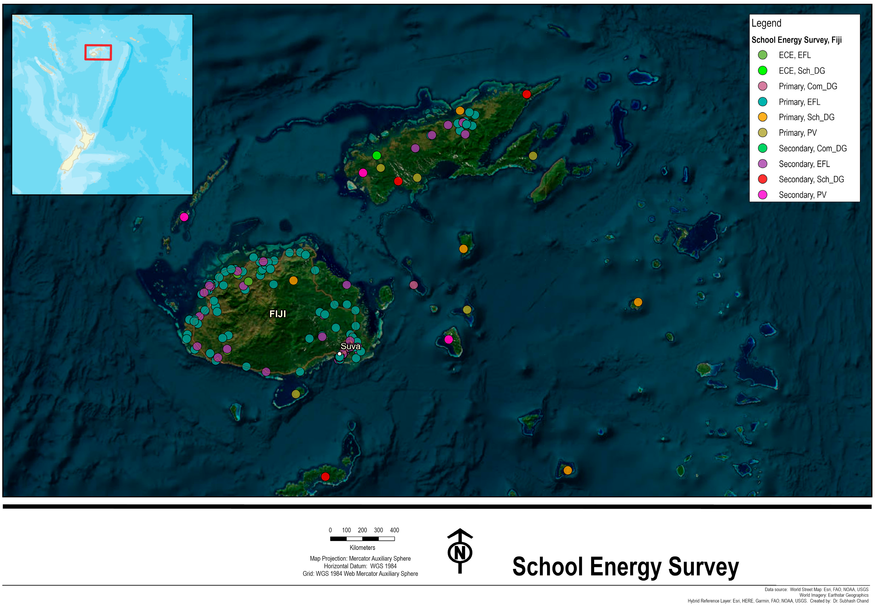
2.2. Running the Questionnaire Survey

Once MEHA’s approval for conducting the research was sought, a key person at MEHA was liaised with to decide how best to reach schools around Fiji. The study used a random sampling design similar to Zhou et al. [48]. There was a second wave of COVID-19 in Fiji at the beginning of 2022, so the author conducted an online questionnaire survey. An MS Office form was used to design the questionnaire, and the survey took place between February 2022 and June 2022. To reach the maximum number of schools and obtain a good response rate, divisional officers (central, western, northern, and eastern) and district officers in each division, as shown in Figure 1a, were contacted via email and phone contact details given by the Policy unit in MEHA. Schools in Fiji are in rural and urban communities, and for some rural community schools internet access is not stable, so 3 versions of the questionnaire were prepared: (i) an online form, (ii) an MS Word copy, and (iii) a pdf copy of the form. This made it easy for schools to participate in the survey. This is also similar to the multi-mode survey that Al Qadi et al. [49] used in their study. Once district officers were contacted, the 3 modes of the questionnaire were explained, and district officers were requested to email all the school heads in their districts. Reminders (emails and numerous phone calls) were also made to district officers and divisional officers to remind schools to participate in the survey. Email attachments with filled forms and online responses were received. The responses attached to emails were later transferred to the online form so that all responses were collated and stored in one place.

2.3. Data Screening and Analysis

By the end of June 2022, 173 responses were collected from schools around Fiji, as shown in Figure 2. From the data collected, the information was filtered and cleaned using MS Excel (Office 365). Missing values were not taken into data analysis and removed using the listwise function in IBM SPSS 27 software. Hong et al. [24] cleaned and filtered their data to be used in ANN models, while the different types of missing data and how to deal with missing data has been explained by Bennett [50], where removal of cases was one of the ways of dealing with missing values. From the wide range of data that were collected to analyze, the schools were clustered as seen in Figure 1b. Because of dispersed islands in Fiji, schools have different power sources—grid-connected schools and off-grid schools. Most schools have grid-connected electricity provided by the only power utility company in Fiji (Energy Fiji Limited (EFL)) while others have off-grid electricity, which is either provided by solar photovoltaics or solar lights (PV), a school’s own diesel generator (Sch_DG), or a community diesel generator (Com_DG). The schools were further categorized into ECE, primary, and secondary schools and categorized as small-, medium-, or large-sized depending on their numbers of students as defined by the MEHA. Descriptive statistics for electricity demand, electricity cost, and school building characteristics were determined similarly to other researchers. For instance, average energy consumption was provided as a function of occupancy level in Carpino et al. [51], and Troup et al. [52] used the median value of total EUI to highlight that the median increases with an increasing building envelope that corresponds to cooling loads. Im et al. [53] presented data using central tendency (mean, mode, median), variability using box plots, and standard deviation, and Wang et al. [54] used frequency analysis, average, median, and coefficient of variance to present data.

The electricity utilization index (EUI_elec) was determined using Equations (1) and (2) as shown in Chung and Yeung [9].

$$EU{I}_{elec}=\frac{Electricity Demand \left(\mathrm{kWh}\right)}{floor area \left({\mathrm{m}}^2\right)}$$

(1)

$$EU{I}_{elec}=\frac{Electricity demand \left(\mathrm{kWh}\right)}{student number}$$

(2)

2.4. Regression Analysis

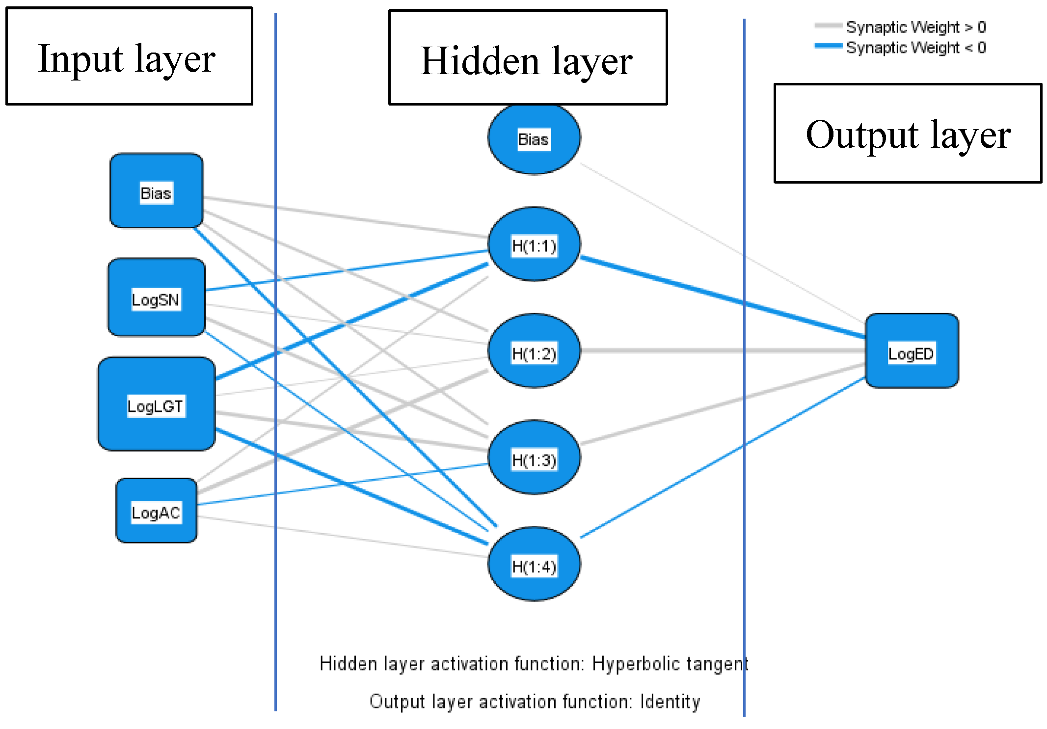
Linear regression models using multiple independent variables were used to predict the electricity demand of grid-connected schools using IBM SPSS 27, similar to the work of many other researchers, as discussed in Section 1. MLR models examine the relationship between the independent and dependent variables and help identify which independent variables account for the most variance in the outcome variable [55]. Regression methods are simple to use, need fewer computing resources than other statistical techniques, and have acceptable prediction accuracy [49], but they are unable to deal with non-linear relationships [56]. Of all the schools that responded to the survey, 154 (89%) were connected to the grid. Box plots was used to identify the outliers. Altogether, 15 outliers were identified for the grid-connected schools. Upon scrutinizing the outlier data, it was found that the two most extreme outliers were schools that had some students with hostel accommodation and the boarders’ electricity bill was included in the school’s electricity bill. For these two outliers, record numbers 149 and 101 were deleted from the entry and not included in the regression analysis. For the mild outliers, it was seen that these were mostly large and medium schools that had high electricity consumption compared to the rest of the schools. It was decided to keep these values. Another school (record number 24) was taken out after running the regression model and obtaining a large maximum Cook’s distance for this school record, indicating an outlier.

After removal of outliers, electricity demand (ED) is taken as the dependent variable while age of schools (Age), number of classrooms (CN), floor area (FA), number of buildings (BN), number of air conditioners (AC), number of students (SN), number of lights (LGT), and number of teachers (TN) were considered as independent variables. To select variables in multiple linear regression, Pearson’s correlation coefficient shown in

Table 1. Pearson’s correlation coefficient of different variables.

	ED	Age	SN	FA	CN	BN	LGT	AC	TN
ED	1.000	0.003	0.735	0.601	0.708	0.216	0.793	0.746	0.854
Age	0.003	1.000	0.050	−0.076	−0.037	−0.175	−0.106	−0.070	−0.068
SN	0.735	0.050	1.000	0.509	0.884	0.196	0.672	0.643	0.828
FA	0.601	−0.076	0.509	1.000	0.573	0.150	0.495	0.543	0.534
CN	0.708	−0.037	0.884	0.573	1.000	0.220	0.657	0.697	0.853
BN	0.216	−0.175	0.196	0.150	0.220	1.000	0.218	0.138	0.304
LGT	0.793	−0.106	0.672	0.495	0.657	0.218	1.000	0.699	0.755
AC	0.746	−0.070	0.643	0.543	0.697	0.138	0.699	1.000	0.763
TN	0.854	−0.068	0.828	0.534	0.853	0.304	0.755	0.763	1.000

was scrutinized. It was seen that the age of the school and number of buildings in the school had poor Pearson’s correlation coefficients of 0.003 and 0.216, respectively. Then, considering collinearity, the number of classrooms had a strong correlation with the number of students (0.884) and the number of teachers had strong correlation with the number of students (0.828). Hence, the number of lights, number of air conditioners, number of students, and floor area were considered as independent variables.

Out of the 151 data points, regression modeling took only 75 data points because of missing values for some variables for different schools. These missing values were mainly for electricity demand, floor area, number of lights, and number of air conditioners because some schools did not respond to this question in the questionnaire. In past studies, it has been seen that there are a range of data points that researchers have used to build predictive models. For instance, Alshibani [32] used 352 datapoints to construct neural network models where the optimum model had an R² value of 97.7%, while Veiga et al. [57] used 48,000 samples to construct predictive models for building energy use and obtained R² values between 84% and 97% for different models. Interestingly, for a study to predict Thailand’s annual electricity consumption, Panklib et al. [35] used 17 datapoints to train its MLR and ANN model and used 3 data points for model testing, where they got R² value of 96% and 99% for MLR and ANN, respectively. Hence, for this current study, it is inferred that 75 datapoints are sufficient to yield statically significant predictive models. It should also be noted that Fiji is a small island country that has 907 primary and secondary schools in total, where the majority of ECE schools are attached to primary schools, and their electricity cost is included in the primary school’s electricity bill. Hence, using 75 schools data for analysis out the 907 schools yields an 11% margin of error with a 95% confidence interval using the formula provided at [58].

Finally, 55 data points (73% of the 75 data points) were used for constructing regression models while 20 data points were used in testing the model performance. The training-to-testing ratios vary, and Veiga et al. [57] reports 80% of the datapoints being used for training the model while 20% of the datapoints were for testing. However, they do not provide information on how the testing datapoints were selected. Alsibani [32] randomly selected 60% of the data points for training the model, 20% for selection, and 20% for testing, while Yuan et al. [31] used 70% for training and 30% for validation and testing that were also randomly selected. For the current study, the training and testing datapoints were based on random selection, where in both (training and testing) datasets representations of different classifications (primary and secondary of different student numbers) of school are present. The training dataset had 3 large-, 20 medium-, and 11 small-sized primary schools and 5 large-, 7 medium-, and 9 small-sized secondary schools. The testing dataset had 2 large-, 3 medium-, and 5 small-sized primary schools and 2 large-, 4 medium-, and 4 small-sized secondary schools.

The general form of the MLR is given by Equation (3). Log forms of variables were used because it provided a better linear relationship as seen in Section 3.2.

logED = β₀ + β₁ logSN + β₂ logFA + β₃ logAC + β₄ logLGT + ε

(3)

where indicators are as follows:

β₀ is the constant of the equation;

β₁ is the coefficient of the logarithm of number of students (logSN);

β₂ is the coefficient for the logarithm of floor area (logFA);

β₃ is the coefficient for the logarithm of the total number of air conditioners (logAC);

β₄ is the coefficient for the logarithm of number of lights (logLGT);

ε is the error term of the equation;

logED is the logarithm of electricity demand (ED).

The number of classrooms is not taken as an independent variable in Equation (3) because it is collinear with the number of students. Therefore, the dependent variable is logED while the independent variables (IVs) are logFA, logSN, logLGT, and logAC.

The predictive power of a multiple regression model can be assessed using the R² value, which measures how close the data are fitted to the fitted regression line [59]. In addition, p-value was used to determine if the independent variable has a statistically significant effect on the dependent variable. This study’s significance level was set at 0.05, similar to what Rinaldi et al. [46] had chosen in their research. If the p-value was less than or equal to 0.05, then the independent variable is statistically significant and if the p-value was more than 0.05, then that independent variable was dismissed.

For any regression modeling, certain assumptions (sample size, normal distribution, absence of outlier, linear relationship, absence of multi-collinearity, and presence of homoscedasticity) are made [60] and these were checked during linear regression modeling, which is shown in Supplementary Data S2.

2.5. ANN Model

In the analysis of the ANN model in IBM SPSS Statistics 27, Multilayer Sensor (MLP—Multilayer Perceptron, which is most popular amongst the different ANN architectures present [61]) was used. This study used a multilayer feedforward network to establish the neural network using a backpropagation algorithm, similar to Zeng et al.’s [62] work. The data set was partitioned in a manner where 70% of the data points were chosen as training data points while the remaining 30% were testing data points. There were 3 layers in the neural network; the first was the input layer that had the input variables, the second was the hidden layer that was used to train and test the data sets, and the third was the output layer that had the output variable. As an example, the structure of ANN model 12.1 is shown in Figure 3. The “Hyperbolic tangent Function” was used as the activation function of the artificial nerve cells in the input layer, and the “Identity Function” was used in the output layer. Jeong [30] explains in detail the equations that relate the input layer, hidden layer, and output layer.

2.6. Testing Model Performance

Root mean square error (RMSE) and coefficient of determination (R²) were used to estimate the performance of MLR and ANN predictive models using Equations (4) and (5), respectively [31,36].

$$RMSE=\sqrt{\frac{{\sum }_{i=1}^N{\left(E{D}_{pre,i}-E{D}_{obs,i} \right)}^2}{N}}$$

(4)

$$R^2=1-\frac{{\sum }_{i=1}^N{\left(E{D}_{obs,i}-E{D}_{pre,i} \right)}^2}{{\sum }_{i=1}^N{\left(E{D}_{obs,i}-E{D}_{avg} \right)}^2}$$

(5)

where i is the ith school, N is the nth school, ED_obs is the annual electricity consumption of a particular school, ED_pre is the predicted annual electricity consumption from a predictive model, and ED_avg is the average of the observed annual electricity consumption of all schools.

The overall methodology of the study is summarized in Figure 4.

3. Results

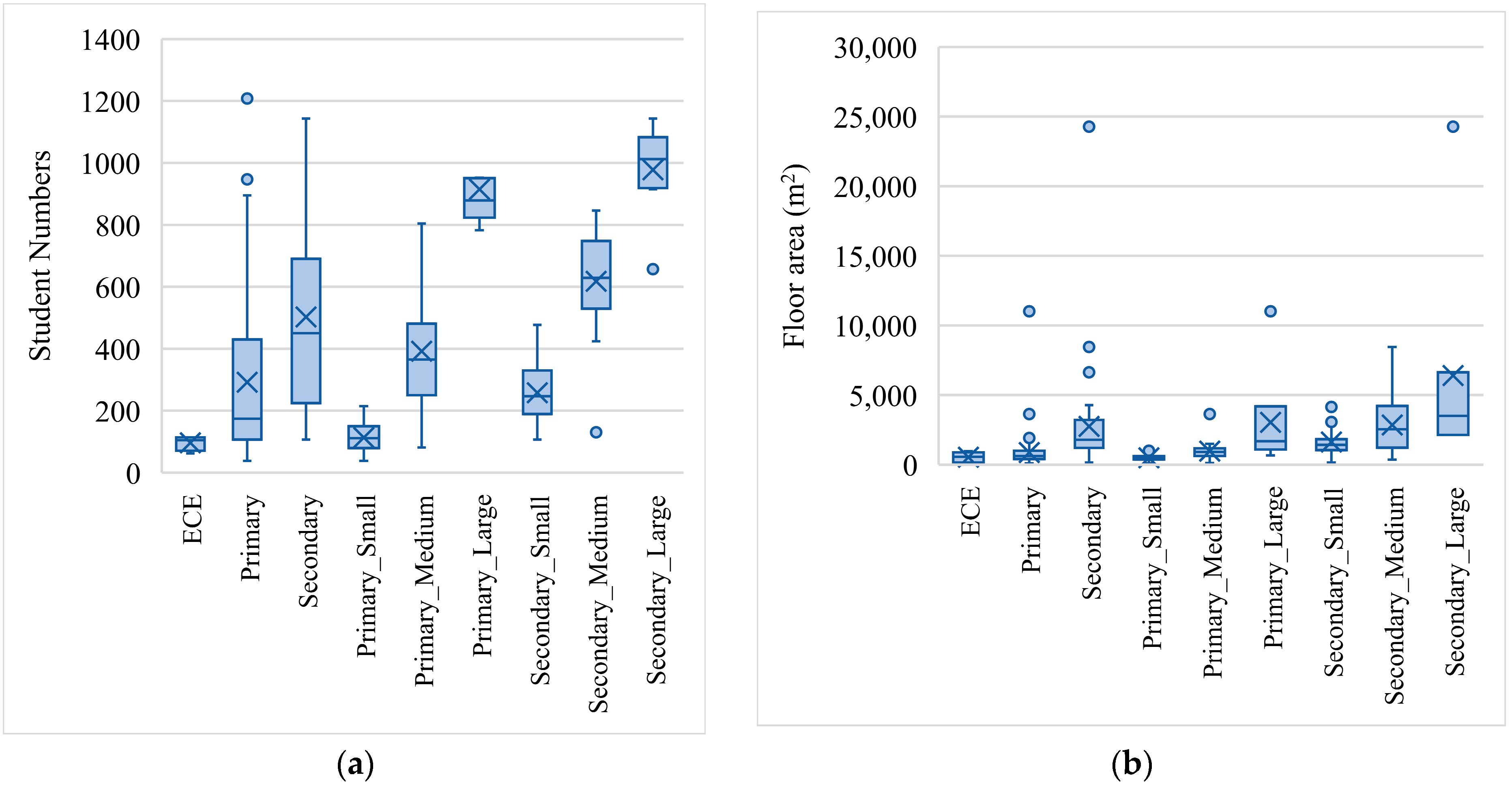
3.1. Descriptive Statistics of the Sampled Schools

A total of 173 responses were received from schools, of which 5 were from standalone ECE, 109 were from primary schools, and 59 were from secondary schools. All the ECE schools were small, while primary and secondary schools were categorized as small, medium, or large. The categorization depended on the number of students for the schools. In terms of the electricity provider, 154 of the sampled schools were grid-connected while the remaining schools were off-grid. This paper will focus on grid-connected schools.

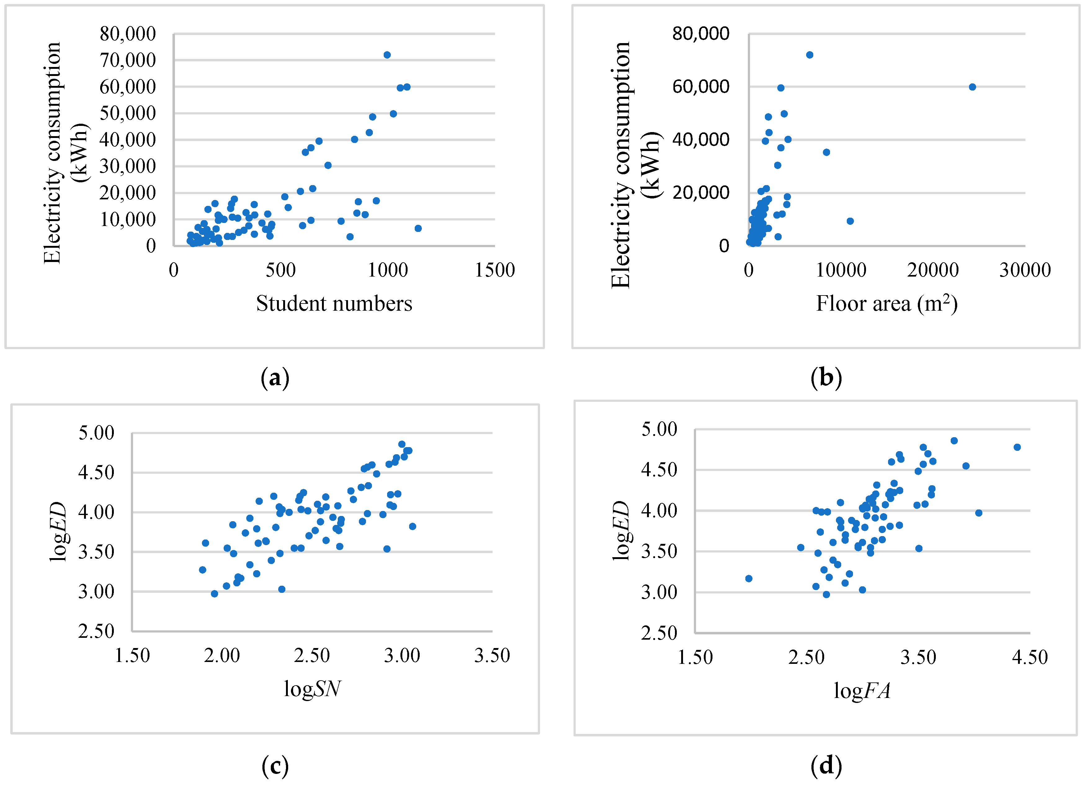
3.1.1. Electricity Consumption of Schools Connected to the Grid

Electricity Fiji Limited (EFL) supplied the primary electricity to a total of 154 school respondents. Out of the 154 schools, there were 4 standalone ECE, 52 secondary, and 98 primary schools. Out of all the primary school respondents, 59 schools reported that ECE was included in their electricity bill, indicating that these primary schools have ECE facilities attached in their school premises.

Box plots of different parameters are shown in Figure 5. Box plots provide information about the distribution of a variable. The middle line of the box represents the median, the lower part of the box represents the lower quartile (Q₁), and the upper part of the box is the upper quartile (Q₃). The mean is represented by the “x” plot in the box. The interquartile range can be found from the difference between Q₃ and Q₁. The whisker above the box represents the maximum value and the whisker at the bottom represents the lowest value. The circled dots in the box plots represent the potential outliers in the data. In schools that participated in the survey, the average number of students in large schools ranged from 800 to 1100, while medium schools ranged from 300 to 700 students and small schools from 100 to 250 students as seen in Figure 5a. Even though numbers of students for secondary and primary schools are comparable, the average annual electricity consumption and its costs are high for secondary in comparison with primary as seen in Figure 5b,c. The electricity demand for ECE schools ranged from 1200 to 1816 kWh/year and primary school electricity demand ranged from 353 to 18,000 kWh/year, while for secondary schools it was 1765 to 72,000 kWh/year. The average annual electricity consumption for secondary schools is around 3–4 times more than primary schools in different categories, and a similar trend is seen for electricity cost in Figure 5d. This could be attributed to the use of air conditioning systems in the specialized rooms.

As seen from Figure 5e,f, the electricity utilization index (EUI_elec) for standalone ECE schools ranged from 1.26 to 37.50 kWh/m²/year or 10.53 to 18.92 kWh/student/year. For primary schools, it ranged from 0.83 to 68.25 kWh/m²/year or 4.43 to 60.47 kWh/student/year. Secondary schools had a much higher EUI_elec; it ranged from 0.54–118.15 kWh/m²/year and 4.17–11.47 kWh/student/year. Overall, schools in Fiji have on average 10.52 kWh/m² or 29.92 kWh/student, while the electrical energy consumption in European schools ranged from 7 to 66 kWh/m² according to the literature [5]. Elementary schools in Korea have energy consumption ranging from 820 to 1080 kWh/student [5]. For schools in China, the average electricity utilization index was 36.07 kWh/m²/year [27]. Overall, for Fijian schools, the average EUI_elec of different schools is below 15 kWh/m² except for medium-sized secondary schools. However, large-sized secondary schools have an average of 12.62 kWh/m² while ECE has 14.09 kWh/m² of electricity consumption. For two secondary schools, the EUI_elec ranges between 80 and 120 kWh/m². For the electricity consumption per capita, it is seen that Fijian secondary schools have a relatively higher (2–3 times more) EUI_elec compared to primary and ECE schools.

3.1.2. Building Characteristics for Fijian Schools

From the schools that participated in the survey, the average floor area of secondary schools (2780 m²) is relatively bigger than other clusters of schools. The average floor area of large grid-connected secondary schools (6100 m²) is almost twice that of large grid-connected primary schools and medium grid-connected secondary schools. It is seen that medium and large secondary schools have a high number of air conditioning systems in use. The data for the exact number of fans in schools was not collected; instead, a range of fans was collected. Almost 62% of schools responded that they had more than ten fans. On average, most grid-connected schools had double-story buildings while ECE schools had a single story and a few small- and medium-sized primary schools had single-story buildings.

3.2. MLR Models for Predicting Electricity Demand for Grid-Connected Schools

The relationship between the dependent variable, electricity demand (ED), and independent variables was plotted to determine the linear relationship. A linear relationship was observed but the majority of the data points were clustered in one corner of the graph as seen from sample graphs for electricity consumption plotted against student numbers and floor area as shown in Figure 6a,b. Logarithmic relations between the dependent and independent variables were explored to obtain a clearer linear relationship between the variables, similar to Sharp [63]. As a result, from Figure 6c–f it is now evident that there is a stronger linear relationship between the logarithm of electricity demand and the logarithms of four independent variables. Other assumptions for regression modeling are shown in Supplementary Data S2.

Three methods of linear regression were carried out, Enter, Stepwise, and Backward, to construct regression models for predicting electricity demand for grid-connected schools. The “Enter” method is where the user, through their judgment, selects the IVs to build the regression model. In the Backward method, the algorithm in SPSS first selects all the IVs in predicting logED and then successively removes non-significant IVs. In the Stepwise method, the IVs are chosen based on a series of automated steps, where at every step the candidate variables are evaluated, one by one, typically using the t statistics for the coefficients of the variables being considered [64].

In view of the R² values in

Table 2. Model summary for estimating electricity demand for all grid-connected schools.

Method	Number of Cases	Input Variables, IVs		Model Summary			ANOVA
			Equation Number	R2	Durbin–Watson	ε	F—Ratio Regression df Residual df	p-Value
Enter	55	IVs: logLGT, logSN, logAC, and logFA	(6)	0.733	1.666	0.23903	34.366 4 50	0.000
Backward	55	IVs: logLGT, logSN, and logAC	(7)	0.733	1.676	0.23697	46.579 3 51	0.000
Stepwise	55	IV: logLGT	(8a)	0.624		0.27571	87.908 1 53	0.000
	55	IVs: logLGT, logSN	(8b)	0.705		0.24659	62.076 2 52	0.000
	55	IVs: logLGT, logSN, and logAC	(8c)	0.733	1.676	0.23697	46.579 3 51	0.000
Enter	55	IV: logSN	(9)	0.504	1.840	0.31665	53.825 1 53	0.000
	55	IVs: logSN and logFA	(10)	0.587	1.736	0.29166	36.959 2 52	0.000
	55	IVs: logSN, logFA, and logLGT	(11)	0.706	1.502	0.24843	40.848 3 51	0.000

, for the “Enter” method, 50–70% of the variation in the outcome variable is explained by the regression models (6, 9, 10, and 11), while for the Stepwise and Backward methods, 73.3% of the variation is explained by the model. In the Stepwise regression, the R² value increases as more independent variables (IV) are added to the model. From the ANOVA column, results indicate that the models were a significant predictor of the outcome variable, logED, as the p-value is 0.000, which is less than 0.05.

Equation (6) has all four IVs included, but it can be seen from

Table 3. Regression coefficients for predicting electricity demand for grid-connected schools.

	Equation	Max Cook’s Distance	β0	β1 (logSN)	β2 (logFA)	β3 (logAC)	β4 (logLGT)
Enter
Unstandardized	(6)		1.609	0.423	0.045	0.272	0.571
t-stat			5.116	2.929	0.353	2.256	3.447
p-value			0.000	0.005	0.725	0.028	0.001
Standardized coefficient Beta				0.263	0.113	0.236	0.390
Cook’s distance		0.191
Backward
Unstandardized	(7)		1.646	0.443		0.275	0.600
t-stat			5.616	3.364		2.303	4.232
p-value			0.000	0.001		0.025	0.000
Standardized coefficient Beta				0.316		0.226	0.447
Cook’s distance		0.233
Stepwise
Unstandardized	(8a)		2.096				1.060
t-stat			10.639				9.376
p-value			0.000				0.000
Standardized coefficient Beta							0.790
Unstandardized	(8b)		1.328	0.506			0.762
t-stat			4.937	3.776			5.949
p-value			0.000	0.000			0.000
Standardized coefficient Beta				0.361			0.568
Unstandardized	(8c)		1.646	0.443		0.275	0.600
t-stat			5.616	3.364		2.303	4.232
p-value			0.000	0.001		0.025	0.000
Standardized coefficient Beta				0.316		0.226	0.447
Cook’s distance		0.233
Enter
Unstandardized	(9)		1.397	0.996
t-stat			4.047	7.337
p-value			0.000	0.000
Standardized coefficient Beta				0.710
Cook’s distance		0.167
Enter
Unstandardized	(10)		1.056	0.626	0.410
t-stat			3.154	3.695	3.236
p-value			0.003	0.001	0.002
Standardized coefficient Beta				0.446	0.391
Cook’s distance		0.170
Enter
Unstandardized	(11)		1.279	0.477	0.063		0.719
t-stat			4.420	3.223	0.479		4.546
p-value			0.000	0.002	0.634		0.000
Standardized coefficient Beta				0.340	0.060		0.536
Cook’s distance		0.142

that the logFA coefficient is not statistically significant as the p-value is 0.725, which is more than 0.05. So, it is best to drop this IV from the regression model. Hence, in Equations (7) and (8a–c), logFA is not considered in the regression model using the Backward and Stepwise methods. Equations (7) and (8c) are the same because Stepwise regression includes Forward and Backward regression. These equations have the highest R² value compared to all the built regression equations.

Overall, Table 2 and Table 3 provide regression models for estimating the electricity demand where the models explain around 50–73% of the variation. To achieve better R² values, ANN models are explored in the next sub-section.

3.3. ANN Models for Predicting Electricity Demand and Performance Testing

The different parameters collected from various grid-connected schools were taken as inputs and the electricity demand was taken as the output variable in the ANN model. The data was divided into sets for training the neural network and testing the ANN model. For the ANN method, different combinations of input variables were trialed in an attempt to obtain better model predictions. For models 12.1–12.6, logarithm transformations of variables were used, similar to MLR, but school types (ST) and school categories (SC) which were nominal data type were also used as independent variables. For the same data set (75 datapoints), the original forms of variables were taken and modeled again which is shown in models 13.1–13.4. There was an improvement in the R² value for models 12 to 13, but in model 13 the RMSE is high. So, it was decided to consider all the 151 datapoints in an ANN model from which 100 data points were taken in models 14.1–14.15. All the variables were selected in 14.2 after which variables were gradually dropped to see the R² value. In addition, the dependent variables were taken in two forms; one was logED and the other form was in its original form, annual electricity demand (ED). Because the MLR method has a set of assumptions to be met, the dependent and input variables were transformed into logarithm forms. However, an ANN has the ability to learn or train itself and use either linear or non-linear structures to predict; it does not have any pre-conditions that have to be met before the modeling. Hence, for ANN models, different forms of input and output variables are taken as shown in

Table 4. ANN models with different input variables and two forms of output variable.

Model	Model No.	Total Data Points	Inputs	Neurons in Hidden Layer	Output Variable	R2	RMSE
MLR		75	logSN, logAC, logLGT		logED	0.7522	0.2248
ANN	12.1	75	logSN, logAC, logLGT	4	logED	0.7440	0.2285
ANN	12.2	75	logSN, logAC, logLGT, logFA	3	logED	0.7541	0.2240
ANN	12.3	75	ST, SC, logLGT, logFA, logAC, logSN, Age	3	logED	0.7195	0.2392
ANN	12.4	75	ST, SC, logLGT, logFA, logAC, logSN	2	logED	0.8400	0.1807
ANN	12.5	75	ST, SC, logLGT, logAC, logSN, Age	5	logED	0.8228	0.1902
ANN	12.6	75	ST, SC, logLGT, logAC, logSN	4	logED	0.7769	0.2133
ANN	13.1	75	ST, SC, LGT, FA, AC, SN, Age	3	ED	0.8398	6203.7
ANN	13.2	75	ST, SC, LGT, FA, AC, SN	3	ED	0.8180	6612.2
ANN	13.3	75	ST, SC, LGT, AC, SN	4	ED	0.8026	6886.2
ANN	13.4	75	ST, SC, LGT, AC, SN, Age	3	ED	0.8365	6266.9
ANN	14.1	100	ST, SC, LGT, FA, AC, SN, Age, TN, FN, CN, BN	5	ED	0.8905	280.51
ANN	14.2	100	ST, SC, LGT, FA, AC, SN, Age, TN, FN, CN, BN, BT	4	ED	0.9350	150.33
ANN	14.3	100	ST, SC, LGT, FA, AC, Age, TN, FN, CN, BN, BT	2	ED	0.9147	105.73
ANN	14.4	100	SC, LGT, FA, AC, SN, Age, TN, BT, FN, CN, BN	3	ED	0.8856	170.37
ANN	14.5	100	ST, SC, LGT, FA, AC, SN, Age, TN, BT, FN, CN	2	ED	0.9196	86.231
ANN	14.6	100	ST, SC, LGT, FA, AC, Age, TN, FN, CN, BN	2	ED	0.9467	36.769
ANN	14.7	100	ST, SC, LGT, FA, Age, TN, FN, CN, BN	5	ED	0.9526	109.26
ANN	14.8	100	ST, SC, LGT, FA, AC, SN, TN, BT, FN, CN, BN	6	ED	0.9282	233.00
ANN	14.9	100	ST, SC, LGT, FA, TN, FN, CN, BN	4	ED	0.9528	59.358
ANN	14.10	100	ST, SC, LGT, FA, Age, TN, FN, CN	4	ED	0.9261	4.1990
ANN	14.11	100	ST, SC, LGT, FA, AC, Age, TN, FN, CN	2	ED	0.9541	447.56
ANN	14.12	100	LGT, FA, SN, AC	4	ED	0.8576	356.17
ANN	14.13	100	LGT, FA, AC, SN, Age, TN, FN, CN, BN, BT	3	ED	0.9412	124.55
ANN	14.14	100	LGT, FA, AC, SN, Age, TN, FN, CN	4	ED	0.9215	326.66
ANN	14.15	100	ST, SC, LGT, FA, AC, SN, Age, TN, FN, CN	3	ED	0.9000	66.799

Note: ST—school type, SC—school category, Age—school age, TN—number of teachers, CN—number of classrooms, FN—number of floors, BN—number of buildings, BT—type of building. The highlighted models are the optimum ANN model.

which is discussed in the next sub-section. For log transformations of variables, 75 datapoints were taken and for the original form of variables, 100 data points were considered in the ANN model as seen in Table 4. For log transformation, the number of datapoints is less because some schools do not have AC or have one air conditioning system and this makes less datapoints for log-transformed variables. The highlighted models are the optimum ANN models for predicting electricity demand by considering their R² and RMSE. It was ensured that optimum models have high R² values while their corresponding RSMEs are low.

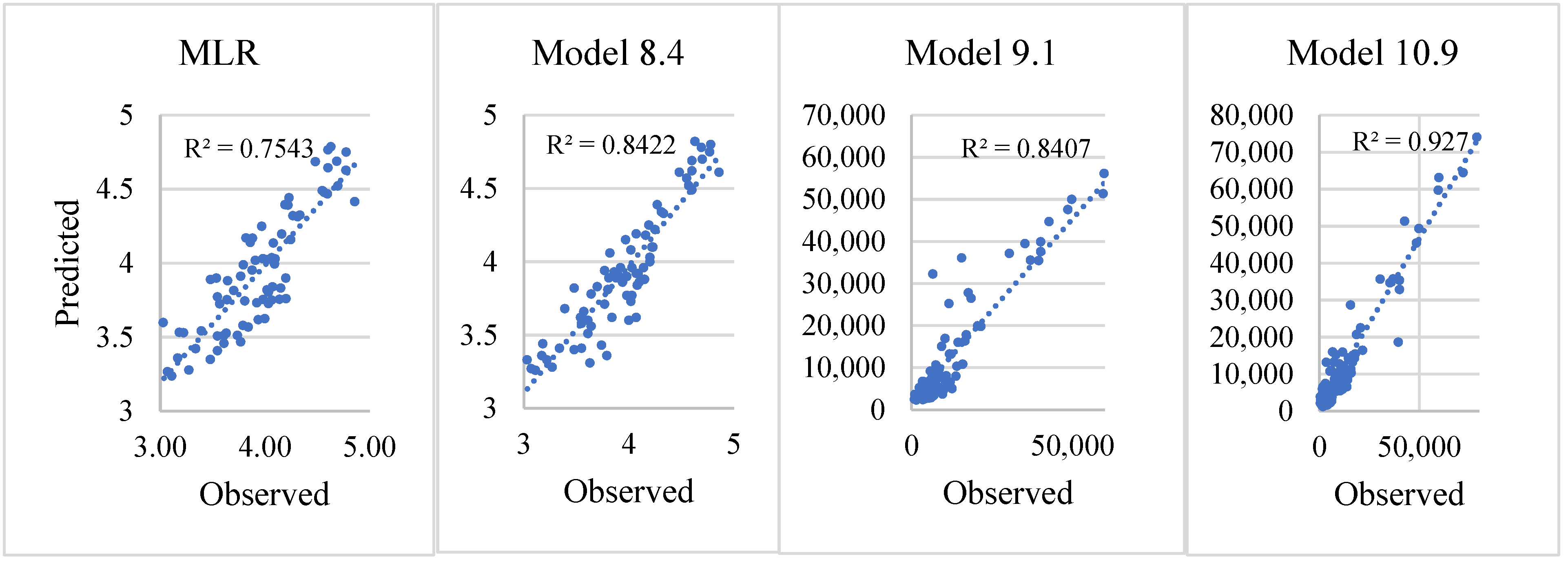
3.3.1. Testing Performance of MLR and ANN Models

Table 4 presents the inputs, the number of neurons in one hidden layer, and the performance parameters (R² and RMSE) of each model. From the definition of R² which is 1 minus the relative error, it can be seen that when many input variables are taken, the R² value improves; that is, the relative error of the prediction model decreases. For the MLR model, R² ranged from 50 to 70% as seen in the previous section. For ANN models, it can be seen that when the output variable is logED and the same range of data points is taken as in the MLR analysis data set, then the R² value improves and goes up to 84% (model 12.4), which is an improvement compared to the MLR method. However, when using the same dataset but the output variable is not transformed, that is, taking the output variable as ED, the best ANN model still measures an R² value around 84% (model 13.1) as seen in Table 4. So, it can be inferred that in ANN models whether one uses a transformed output or the output in its original form, the model performance is the same. To further improve the predictions, all the data that was obtained during the data collection method was taken into the ANN model and the schools that had missing values were excluded from the modeling. However, the extreme values and the outliers were included in the modeling.

Therefore, considering the set of ANN models (14.1 to 14.15), the R² value ranges from 85.8 to 95.4% which is a significant improvement from the MLR predictions, but it was still not able to reach close to 99%. Yuan et al. [31] reported an R² value ranging from 95 to 99% for ANN models used for predicting hourly electricity consumption at a university campus while the authors of [35] reported an R² value of 96% from the MLR model and 99% for the ANN model for predicting annual electricity consumption in Thailand. The R² and RSME were 89% and 11.69 kWh/m², respectively, for the regression model and 99% and 2.61 kWh/m², respectively, for the ANN model in the study conducted by Quevedo et al. [20] on energy consumption at a university building. Similarly, in Veiga et al. [57], for MLR models the R² ranged from 84% to 90% and RSME ranged from 8.4 to 10.95 kWh/m²/year for bank buildings in Brazil while ANN models had an R² value ranging from 88% to 97% and RSME ranging from 4.34 to 9.46 kWh/m²/year. In Yuan et al. [31], the RSME was reported to range from 6.5 to 48.9 kWh while, in the current study, the RSME for models 14.1 to 14.15 using ANN was 4.2 to 356 kWh as shown in Table 4. The difference in the current study’s R² and RSME compared to other published literature is a slight decrease in R² values and increase in the RSME values, which could be due to the number of datapoints taken during modeling and the independent variables taken during model construction.

According to Mohammed et al. [22] and Islam et al. [65], plotting predicted values against the actual data would show the correlation between the predicted and the actual values. The closer the R² value is to 1, the better the regression model. By plotting the graph shown in Figure 7 of predicted against observed values for the models selected in Table 4, it is seen that ANN models predict better than MLR models, and when input parameters increase, the ANN model predicts better.

Similarly, it is seen that for the most optimum predictions, the R² value is the largest while the RMSE is the smallest. RMSE has the unit of the output variable and measures how far predictions deviate from measured or observed values using Euclidean distance [66]. The smaller the RMSE value, the better the model is at predicting the output variable. Comparing the models for predicting logED, the RMSE of MLR is 0.2248 while for models using ANN the RMSE is relatively less, with the lowest RMSE of 0.1807 as seen in Table 4. In addition, comparing the models for predicting ED where different numbers of data points were taken, it is seen that for modeling with 75 data points, RMSE is significantly higher while for modeling with 100 data points, the model yields relatively less RMSE. This could also be because a higher number of input variables are considered in the larger dataset.

Further, it is seen that the lowest RSME is for model 14.10, which has eight independent variables; the highest R² is for model 14.11, but this model obtained a relatively higher RMSE in comparison to model 14.10. To strike a balance between the two performance indices, model 14.9 could be a better predictor model, as it has both a higher R² (95.3%—second highest) and a relatively lower (59.4 kWh/year—second lowest) RMSE.

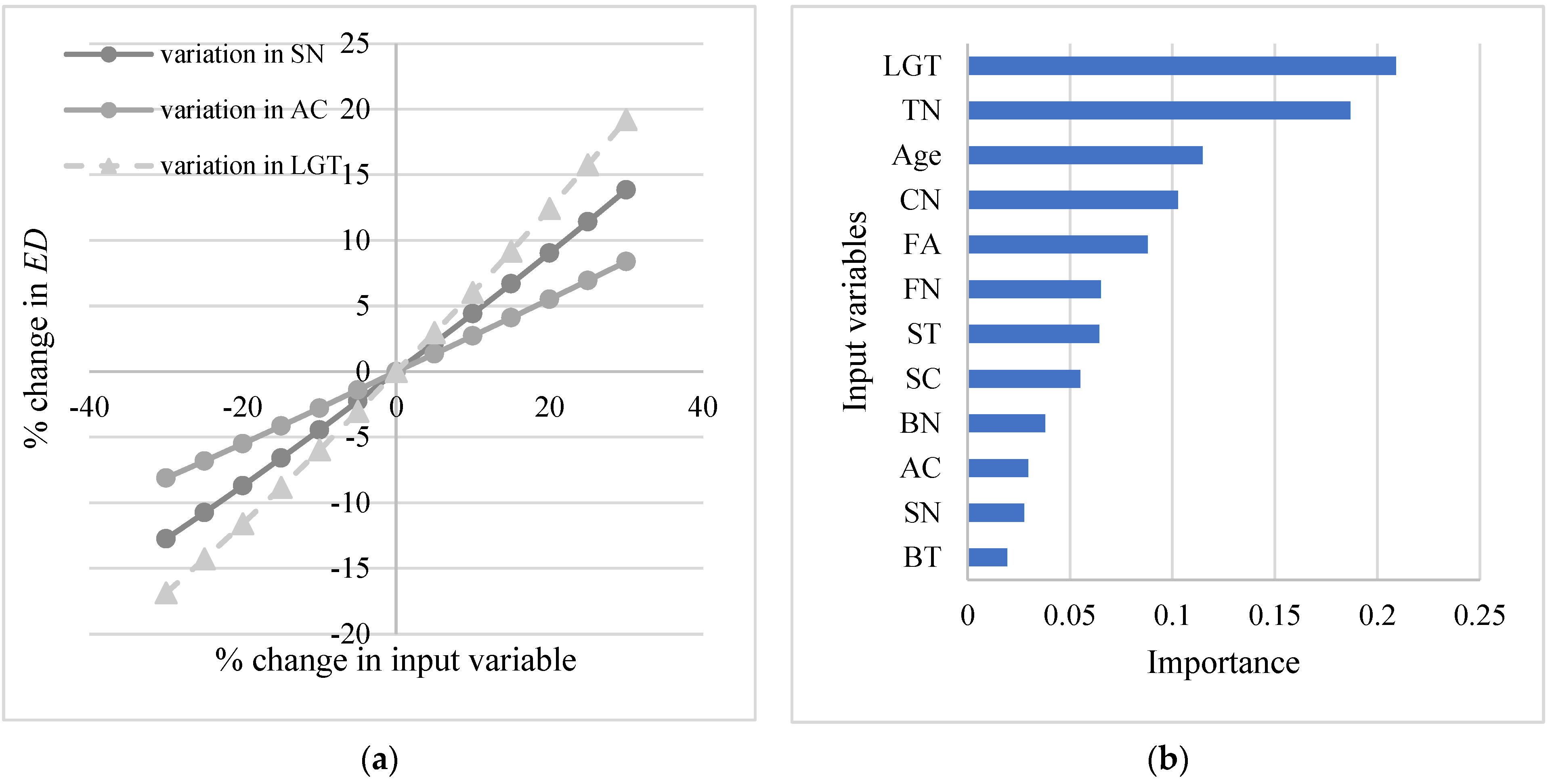
3.3.2. Importance of IVs That Affect School Electricity Demand

Sensitivity analysis was performed to study which independent variable impacted the outcome variable the most in the MLR model. Equation (8c) was used to calculate the predicted electricity demand from student number (SN), number of lights (LGT), and number of air conditioners (AC). The mean values of the three IVs were taken and the mean of each IV was varied (while keeping the other two IVs constant) in steps of 5% from above and below the mean until there was a 30% change. The % change in the electricity demand was noted. From Figure 8a, it is seen that the number of lights in the schools had the steepest line, indicating that it had the most impact on the electricity demand. This was followed by the student number and number of air conditioning units in the schools. This means that the more lights a school has, the greater it will affect the electricity demand. The same thing is also inferred from Table 3 when we look at the standardized coefficient beta. It is seen that for Equation (8c), logLGT has the highest standardized coefficient beta, followed by logSN and then logAC. For instance, electricity demand increases by 12% when the number of lights increases by 20% and the electricity demand increases by 9% when the student number increases by 20%. Also, for a 20% increase in the number of AC units, the electricity demand increases by 5.5%.

In addition, the ANN models in SPSS also presented the importance of different input variables for each model. As an example, Figure 8b shows how important different independent or input variables are to predict the output variable—in this case, the annual electricity demand in kWh. It is seen that the number of lights and number of teachers have relatively high importance in predicting the annual electricity demand.

4. Discussions

4.1. Implications of the Current Study

The regression model built shows that the number of lights, students, and air conditioning systems have a significant impact on the electricity demand of schools in Fiji. Similar results were also shown in the study by Litardo et al. [67], where they found that cooling degree days and number of occupants affected the annual energy consumption of university classrooms. In addition, Yuan et al. [68] found that occupancy densities of classrooms affected the electricity consumption of air conditioners, while building age was also a significant factor affecting energy usage for [22]. The results imply that schools need to look at the way they use lights and air conditioning systems. Also, from ANN models, building type (whether concrete, wooden, or both), type of school (whether primary or secondary), and category of school (whether small, medium, or large) also affect the electricity demand. Schools should effectively monitor their electricity consumption and keep records of their monthly bills and kWh consumption. There should be more awareness in schools of how to conserve electricity, as it comprises one of the major operating costs of schools; the annual electricity bill for a primary school can go as high as FJD6000, while for secondary schools it can go as high as FJD21,000.

There needs to be a dedicated energy manager or coordinator at individual schools who can coordinate electricity monitoring, keeping of records, raising awareness of conservation, and implementing low-cost measures to reduce electricity consumption, especially from lights and air conditioning systems. There can be labels to switch off lights and air conditioning systems when the room is empty or if the weather is favorable. For instance, using natural ventilation is recommended by Dimoudi and Kostarela [69] to promote energy saving and establishing comfortable conditions within buildings. Schools can consider replacing inefficient lights with more efficient ones such as replacing compact fluorescent tube lights with LED tube lights. If schools have enough financial resources, they can even consider replacing their existing luminaires with reflector-type luminaires which could reduce the need for higher power ratings of lights. In addition, Lourenco et al. [70] recommend use of natural lighting in buildings as an energy management strategy. For air conditioning systems, schools can ensure that the rooms are properly insulated, that is, there are no broken windows (missing louvres) or gaps around door edges from which cool air can escape, thereby making the air conditioning system consume more electricity. Schools can also consider servicing their existing air conditioning systems regularly to ensure they operate efficiently.

The Ministry of Education can use the findings of this study to design policies and incentives that promote energy efficiency and conservation in schools. It must be realized that to adapt to climate change, to be resilient to climate change, and to mitigate greenhouse gases, there needs to be a behavioral change in end-users. However, behavioral change is a long and slow process. And for it to happen, it should start from the grassroots level, that is, with the younger generation who are future leaders and end-users. A similar view is also shared by Pietrapertosa et al. [71], who highlight and study how the behavior of young students can be influenced by awareness programs through gamification and poster-making competitions. Customized energy management programs needs to be implemented so that there is continuous effort to improve energy performance of schools in the long-term [72]. With the findings of the current study, the Ministry of Education can make it compulsory for schools to create a goal/target for energy reduction through an initial baseline survey. This can be followed up by schools monitoring their electricity consumption, keeping records, and reporting their monthly consumptions annually to the Ministry. This will ensure that all schools can participate in taking individual action in their schools when compared to the currently fewer schools monitoring and raising awareness of conservation. This may result in students taking part in energy reduction initiatives and thus changing their behavior and influencing their peers, family, and relatives. The Ministry of Education, with the Department of Energy, can also provide incentives such as grants for schools, especially those not financially secure, to implement energy efficiency. Also, there can be rewards from the Ministry to schools that share the best practices in reducing their electricity bills and show proof of reduction.

The findings of this study can also inform relevant departments and organizations that are involved in preparing building codes and standards. There can be a section in these documents that set standards on the energy performance of buildings and on how to design energy-efficient buildings that consider lighting and cooling energy demand. For example, lighting design can consider natural lighting, while designing for cooling energy demand can consider designing the orientation of windows that capture natural ventilation during summer and capture heat during winter season.

The Pacific region including Fiji has developed a framework for energy security and resilience for the region that highlights action plans for achieving energy security while minimizing global emissions [73]. Fiji also has updated its nationally determined contributions for emission reductions where energy efficiency is one of the key areas for achieving the targets [42]. This study contributes to data and knowledge on the energy demand for school buildings in Fiji which provides the initial steps for similar work to be carried out for other buildings, such as office spaces, manufacturing industries, public rental homes, apartments, etc. In addition, this work can be replicated by other schools in the Pacific to collect similar data and inform stakeholders on the energy consumption in schools and factors that greatly impact its usage.

4.2. Study Scope, Limitations of Present Study, and Recommendations for Future Study

This study built MLR and ANN models based on the data collected through the online questionnaire survey to predict the electricity demand of Fijian schools. The imputation method was not used for filling the missing values in datasets; instead, these cases were removed during the modeling process. Future research can use the imputation method for filling missing values and then constructing prediction models using deep-learning-based approaches and also other non-linear forms of regression modeling. The major limitation of the MLR method is that it is not able to predict non-linear relationships and a set of assumptions must be met to use the MLR model. Hence, the ANN method was used in this study, which can model non-linear relationships between various independent variables and a dependent variable [74]. However, one limitation of the ANN method is that it is a black box where the user does not have any explicit equation to predict the output, that is, it is unable to explain why and how the solution was found [75]. Only through training with data sets and testing the model is the user able to learn the performance of the model.

In addition, due to missing data from some school responses, prediction models for different school clusters, such as one model for primary school, one for secondary school or small primary schools, etc., were not constructed. Instead, for any school (whether it be ECE, primary, or secondary) or any category (small, medium, or large), MLR and ANN models were built. During the analysis, the author could not obtain grid-connected electricity demand data from the power utility company (EFL). For future study, if electricity demand data is accessed from EFL, floor area data accessed from relevant authorities, and numbers of students accessed from MEHA, then more robust predictive models can be constructed based on the large data set using state-of-the-art methods. Furthermore, due to length constraints, this paper could not investigate in detail the electricity and energy consumption of off-grid schools. Future research will carry out a feasibility study on implementing solar photovoltaic systems for off-grid schools that are using diesel generators and explore a circular economy in schools where alternative cleaner technologies and fuels can be implemented to cater to schools’ cooking energy needs.

Also, to receive a higher response rate for this online survey, the questionnaire was not made very long and hence did not include questions on the power rating of electrical appliances, especially for lights, air conditioning systems, and fans. Therefore, the capacity of different electrical appliances used was not considered while constructing the regression models. So, it is recommended that every school, either through their own initiative or with research performed by external researchers, carry out detailed energy audits. This will help schools keep a record of their electricity use and data can be used for comparative and other energy studies. In addition, for future studies, the behavior of students and teachers can be studied to determine their impact on electricity demand changes. For example, Zhang and Bluyssen [76] surveyed nine primary schools located in different areas in the Netherlands and studied the relationship between the building characteristics and self-reported frequency of teachers’ actions on the school’s energy consumption. They also measured temperature, relative humidity, CO₂ concentration, illuminance, and sound pressure level to study the indoor environmental quality of classrooms. This was similar to the work of Barbosa et al. [77] in their study of a Portuguese school.

Furthermore, building energy management can be promoted in schools for advanced monitoring. Various strategies for building energy management systems are discussed by Hernandez et al. [78] out of which an appropriate one can be adopted in schools. Also, a stochastic and distributed optimal energy management approach for an active distribution network (ADN) with office buildings was proposed by Li et al. [79] for building energy management while Yoon et al. [80] proposes a multiple-power-based building energy management system (MPBEMS) for the efficient management of building energy. To start with, schools in Fiji can be retrofitted with motion or daylight sensors so that lights and fans are switched off when unoccupied or during the daytime. In addition, energy meters that monitor and log data on the energy consumption of major electrical appliances such as lights, fans, and air conditioners can be installed in schools.

Finally, for building cooling, possible renewable energy technologies can be investigated. For instance, Schiboula and Tambani [81] found that a seawater cooling system, deployed at a depth of 700 m in the Caspian Sea, can provide up to 78% energy saving comparing to a conventional cooling system, while seawater to cool chillers was investigated in the urban area of a coastal city [82].

5. Conclusions

This is the first study in Fiji, a small Pacific Island nation, where actual electricity consumption data and related energy and building data were collected by sending out questionnaires to schools around Fiji. Altogether, 173 schools responded to the survey, of which 5 were standalone ECE schools, 109 were primary schools, and 59 were secondary schools. All large primary schools, 98% of medium primary schools, and 83% of small primary schools have electricity provided by EFL, while the rest are off-grid schools. All large and medium secondary schools have grid electricity, while 22% of the small secondary schools have off-grid electricity. The electricity demand for ECE schools ranged from 1200 to 1816 kWh/year, primary school electricity demand ranged from 353 to 18,000 kWh/year, and for secondary schools, it was from 1765 to 72,000 kWh/year. The average annual electricity consumption for secondary schools is around 3–4 times more than primary schools in different categories. The schools’ electricity depends on the number of lights, students, air conditioners, and floor area.

To understand the factors that affect electricity demand in schools, MLR and ANN models were constructed to predict electricity demand for Fijian schools and R² and RMSE were used to test the performance of these models. The most optimum model from MLR was Equation (8c) with an R² of 73.3% and an RMSE of 0.2248. It was seen that ANN models were better predictors of school electricity demand, as the optimum ANN model, 14.9, had the second highest R² of 95.3% and the second lowest RMSE of 59.4 kWh/year. Both ANN and MLR models have shown that light is the most important variable affecting electricity demand while noting that other input variables such as the number of air conditioning systems, school type, and school category are also relatively important.

Hence, if schools want to reduce their electricity cost, they should manage their light and air conditioning usage. The saved energy costs can be utilized by schools for enhancing their teaching and learning activities. This study provides empirical data on electricity consumption in schools and can contribute to better-informed policies to support the development of Fijian schools and building codes and standards as well as the implementation of energy conservation and efficiency measures in schools.

References

1. Amasyali, K.; El-Gohary, N.M. A review of data-driven building energy consumption prediction studies. Renew. Sustain. Energy Rev. 2018, 81, 1192–1205. [Google Scholar] [CrossRef]
2. Wei, Y.; Zhang, X.; Shi, Y.; Xia, L.; Pan, S.; Wu, J.; Han, M.; Zhao, X. A review of data-driven approaches for prediction and classification of building energy consumption. Renew. Sustain. Energy Rev. 2018, 82, 1027–1047. [Google Scholar] [CrossRef]
3. Chemingui, Y.; Gastli, A.; Ellabban, O. Reinforcement learning-based school energy management system. Energies 2020, 13, 6354. [Google Scholar] [CrossRef]
4. Guo, Y.-Y. Revisiting the building energy consumption in China: Insights from a large-scale national survey. Energy Sustain. Dev. 2022, 68, 76–93. [Google Scholar] [CrossRef]
5. Dias Pereira, L.; Raimondo, D.; Corgnati, S.P.; Gameiro da Silva, M. Energy consumption in schools—A review paper. Renew. Sustain. Energy Rev. 2014, 40, 911–922. [Google Scholar] [CrossRef]
6. Airaksinen, M. Energy use in day care centers and schools. Energies 2011, 4, 998–1009. [Google Scholar] [CrossRef]
7. Chung, W.; Yeung, I.M. A two-stage regression-based benchmarking approach to evaluate school’s energy efficiency in different tariff regions. Energy Sustain. Dev. 2021, 61, 15–27. [Google Scholar] [CrossRef]
8. Wang, J.C. Energy consumption in elementary and high schools in Taiwan. J. Clean. Prod. 2019, 227, 1107–1116. [Google Scholar] [CrossRef]
9. Chung, W.; Yeung, I.M.H. A study of energy consumption of secondary school buildings in Hong Kong. Energy Build. 2020, 226, 110388. [Google Scholar] [CrossRef]
10. Ouf, M.M.; Issa, M.H. Energy consumption analysis of school buildings in Manitoba, Canada. Int. J. Sustain. Built Environ. 2017, 6, 359–371. [Google Scholar] [CrossRef]
11. Thewes, A.; Maas, S.; Scholzen, F.; Waldmann, D.; Zürbes, A. Field study on the energy consumption of school buildings in Luxembourg. Energy Build. 2014, 68, 460–470. [Google Scholar] [CrossRef]
12. Stuart, G.; Fleming, P.; Ferreira, V.; Harris, P. Rapid analysis of time series data to identify changes in electricity consumption patterns in UK secondary schools. Build. Environ. 2007, 42, 1568–1580. [Google Scholar] [CrossRef]
13. Samuels, J.A.; Booysen, M.J. Chalk, talk, and energy efficiency: Saving electricity at South African schools through staff training and smart meter data visualisation. Energy Res. Soc. Sci. 2019, 56, 101212. [Google Scholar] [CrossRef]
14. Agarwal, S.; Rengarajan, S.; Sing, T.F.; Yang, Y. Nudges from school children and electricity conservation: Evidence from the “Project Carbon Zero” campaign in Singapore. Energy Econ. 2017, 61, 29–41. [Google Scholar] [CrossRef]
15. Mohamed, S.; Smith, R.; Rodrigues, L.; Omer, S.; Calautit, J. The correlation of energy performance and building age in UK schools. J. Build. Eng. 2021, 43, 103141. [Google Scholar] [CrossRef]
16. Corrado, V.; Ballarini, I.; Paduos, S.; Tulipano, L. A new procedure of energy audit and cost analysis for the transformation of a school into a nearly zero-energy building. Energy Procedia 2017, 140, 325–338. [Google Scholar] [CrossRef]
17. Shailesh, K.; Tanuja, S.; Kumar, M.; Krishna, R.A. Energy consumption optimisation in classrooms using lighting energy audit. In Proceedings of the National Conference on Challenges in Research & Technology in the Coming Decades (CRT 2013), Ujire, India, 27–28 September 2013. [Google Scholar]
18. Borgstein, E.H.; Lamberts, R. Developing energy consumption benchmarks for buildings: Bank branches in Brazil. Energy Build. 2014, 82, 82–91. [Google Scholar] [CrossRef]
19. Vaisi, S.; Varmazyari, P.; Esfandiari, M.; Sharbaf, S.A. Developing a multi-level energy benchmarking and certification system for office buildings in a cold climate region. Appl. Energy 2023, 336, 120824. [Google Scholar] [CrossRef]
20. Quevedo, T.C.; Geraldi, M.S.; Melo, A.P. Applying machine learning to develop energy benchmarking for university buildings in Brazil. J. Build. Eng. 2023, 63, 105468. [Google Scholar] [CrossRef]
21. Kim, T.; Kang, B.; Kim, H.; Park, C.; Hong, W.-H. The study on the Energy Consumption of middle school facilities in Daegu, Korea. Energy Rep. 2019, 5, 993–1000. [Google Scholar] [CrossRef]
22. Mohammed, A.; Alshibani, A.; Alshamrani, O.; Hassanain, M. A regression-based model for estimating the energy consumption of school facilities in Saudi Arabia. Energy Build. 2021, 237, 110809. [Google Scholar] [CrossRef]
23. Bourdeau, M.; Zhai, X.q.; Nefzaoui, E.; Guo, X.; Chatellier, P. Modeling and forecasting building energy consumption: A review of data-driven techniques. Sustain. Cities Soc. 2019, 48, 101533. [Google Scholar] [CrossRef]
24. Hong, S.-M.; Paterson, G.; Mumovic, D.; Steadman, P. Improved benchmarking comparability for energy consumption in schools. Build. Res. Inf. 2014, 42, 47–61. [Google Scholar] [CrossRef]
25. Almeida, A.P.; Sousa, V.; Silva, C.M. Methodology for estimating energy and water consumption patterns in university buildings: Case study, Federal University of Roraima (UFRR). Heliyon 2021, 7, e08642. [Google Scholar] [CrossRef]
26. Nematchoua, M.K.; Yvon, A.; Roy, S.E.J.; Ralijaona, C.G.; Mamiharijaona, R.; Razafinjaka, J.N.; Tefy, R. A review on energy consumption in the residential and commercial buildings located in tropical regions of Indian Ocean: A case of Madagascar island. J. Energy Storage 2019, 24, 100748. [Google Scholar] [CrossRef]
27. Ma, H.; Lai, J.; Li, C.; Yang, F.; Li, Z. Analysis of school building energy consumption in Tianjin, China. Energy Procedia 2019, 158, 3476–3481. [Google Scholar] [CrossRef]
28. Geraldi, M.S.; Ghisi, E. Mapping the energy usage in Brazilian public schools. Energy Build. 2020, 224, 110209. [Google Scholar] [CrossRef]
29. Wu, J.; Lian, Z.; Zheng, Z.; Zhang, H. A method to evaluate building energy consumption based on energy use index of different functional sectors. Sustain. Cities Soc. 2020, 53, 101893. [Google Scholar] [CrossRef]
30. Jeong, K.; Koo, C.; Hong, T. An estimation model for determining the annual energy cost budget in educational facilities using SARIMA (seasonal autoregressive integrated moving average) and ANN (artificial neural network). Energy 2014, 71, 71–79. [Google Scholar] [CrossRef]
31. Yuan, J.; Farnham, C.; Azuma, C.; Emura, K. Predictive artificial neural network models to forecast the seasonal hourly electricity consumption for a University Campus. Sustain. Cities Soc. 2018, 42, 82–92. [Google Scholar] [CrossRef]
32. Alshibani, A. Prediction of the Energy Consumption of School Buildings. Appl. Sci. 2020, 10, 5885. [Google Scholar] [CrossRef]
33. Nsangou, J.C.; Kenfack, J.; Nzotcha, U.; Ngohe Ekam, P.S.; Voufo, J.; Tamo, T.T. Explaining household electricity consumption using quantile regression, decision tree and artificial neural network. Energy 2022, 250, 123856. [Google Scholar] [CrossRef]
34. Zhao, D.; Zhong, M.; Zhang, X.; Su, X. Energy consumption predicting model of VRV (Variable refrigerant volume) system in office buildings based on data mining. Energy 2016, 102, 660–668. [Google Scholar] [CrossRef]
35. Panklib, K.; Prakasvudhisarn, C.; Khummongkol, D. Electricity consumption forecasting in Thailand using an artificial neural network and multiple linear regression. Energy Sources Part B Econ. Plan. Policy 2015, 10, 427–434. [Google Scholar] [CrossRef]
36. Chen, S.; Ren, Y.; Friedrich, D.; Yu, Z.; Yu, J. Prediction of office building electricity demand using artificial neural network by splitting the time horizon for different occupancy rates. Energy AI 2021, 5, 100093. [Google Scholar] [CrossRef]
37. EFL. 2022 Annual Report; Energy Fiji Limited: Suva, Fiji, 2023. [Google Scholar]
38. Joseph, L.P.; Prasad, R. Assessing the sustainable municipal solid waste (MSW) to electricity generation potentials in selected Pacific Small Island Developing States (PSIDS). J. Clean. Prod. 2020, 248, 119222. [Google Scholar] [CrossRef]
39. Prasad, R.D.; Raturi, A. Low carbon alternatives and their implications for Fiji’s electricity sector. Util. Policy 2019, 56, 1–19. [Google Scholar] [CrossRef]
40. Prasad, R.D. Long-Term Energy Planning for Fiji. Ph.D. Thesis, The University of the South Pacific, Suva, Fiji, 2020. [Google Scholar]
41. GoF. Republic of Fiji National Adaptation Plan: A Pathway towards Climate Resilience. Available online: https://www4.unfccc.int/sites/NAPC/Documents/Parties/National%20Adaptation%20Plan_Fiji.pdf (accessed on 24 March 2021).
42. GoF. Fiji’s Updated Nationally Determined Contribution; Government of Fiji. Available online: https://www4.unfccc.int/sites/ndcstaging/PublishedDocuments/Fiji%20First/Republic%20of%20Fiji%27s%20Updated%20NDC%2020201.pdf (accessed on 17 December 2021).
43. Siwatibau, S. Urban Energy in Fiji: A Survey of Suva’s Household, Industrial, and Commercial Sectors; International Development Research Centre: Ottawa, ON, Canada, 1987; Available online: https://idl-bnc-idrc.dspacedirect.org/bitstream/handle/10625/9494/IDL-9494.pdf?sequence=1 (accessed on 20 January 2022).
44. Prasad, R.D.; Raturi, A. Grid electricity for Fiji islands: Future supply options and assessment of demand trends. Energy 2017, 119, 860–871. [Google Scholar] [CrossRef]
45. MEHA. Statistics. Ministry of Education, Heritage and Arts. Available online: https://www.education.gov.fj/statistics/ (accessed on 6 May 2021).
46. Rinaldi, A.; Schweiker, M.; Iannone, F. On uses of energy in buildings: Extracting influencing factors of occupant behaviour by means of a questionnaire survey. Energy Build. 2018, 168, 298–308. [Google Scholar] [CrossRef]
47. Groves, R.M.; Fowler, F.J., Jr.; Couper, M.P.; Lepkowski, J.M.; Singer, E.; Tourangeau, R. Survey Methodology; John Wiley & Sons: Hoboken, NJ, USA, 2011; Volume 561. [Google Scholar]
48. Zhou, T.; Luo, X.; Liu, X.; Liu, G.; Li, N.; Sun, Y.; Xing, M.; Liu, J. Analysis of the influence of the stay-at-home order on the electricity consumption in Chinese university dormitory buildings during the COVID-19 pandemic. Energy Build. 2022, 277, 112582. [Google Scholar] [CrossRef]
49. Al Qadi, S.; Sodagar, B.; Elnokaly, A. Estimating the heating energy consumption of the residential buildings in Hebron, Palestine. J. Clean. Prod. 2018, 196, 1292–1305. [Google Scholar] [CrossRef]
50. Bennett, D.A. How can I deal with missing data in my study? Aust. N. Z. J. Public Health 2001, 25, 464–469. [Google Scholar] [CrossRef] [PubMed]
51. Carpino, C.; Fajilla, G.; Gaudio, A.; Mora, D.; Simone, M.D. Application of survey on energy consumption and occupancy in residential buildings. An experience in Southern Italy. Energy Procedia 2018, 148, 1082–1089. [Google Scholar] [CrossRef]
52. Troup, L.; Phillips, R.; Eckelman, M.J.; Fannon, D. Effect of window-to-wall ratio on measured energy consumption in US office buildings. Energy Build. 2019, 203, 109434. [Google Scholar] [CrossRef]
53. Im, H.; Srinivasan, R.; Fathi, S. Building energy use prediction owing to climate change: A case study of a university campus. In Proceedings of the 1st ACM International Workshop on Urban Building Energy Sensing, Controls, Big Data Analysis, and Visualization, New York, NY, USA, 13–14 November 2019; pp. 43–50. [Google Scholar]
54. Wang, Y.; Wang, F.; Wang, H. Heating Energy Consumption Questionnaire and Statistical Analysis of Rural Buildings in China. Procedia Eng. 2016, 146, 380–385. [Google Scholar] [CrossRef]
55. Washburn, A.; Matsumoto, S.; Riek, L.D. Trust-aware control in proximate human-robot teaming. In Trust in Human-Robot Interaction; Elsevier: Amsterdam, The Netherlands, 2021; pp. 353–377. [Google Scholar]
56. Shao, M.; Wang, X.; Bu, Z.; Chen, X.; Wang, Y. Prediction of energy consumption in hotel buildings via support vector machines. Sustain. Cities Soc. 2020, 57, 102128. [Google Scholar] [CrossRef]
57. Veiga, R.K.; Veloso, A.C.; Melo, A.P.; Lamberts, R. Application of machine learning to estimate building energy use intensities. Energy Build. 2021, 249, 111219. [Google Scholar] [CrossRef]
58. SurveyMonkey. Margin of Error Calculator, Formula, and Examples. Available online: https://www.surveymonkey.com/mp/margin-of-error-calculator/ (accessed on 20 March 2024).
59. Amber, K.P.; Aslam, M.W.; Mahmood, A.; Kousar, A.; Younis, M.Y.; Akbar, B.; Chaudhary, G.Q.; Hussain, S.K. Energy Consumption Forecasting for University Sector Buildings. Energies 2017, 10, 1579. [Google Scholar] [CrossRef]
60. Osborne, J.W.; Waters, E. Four assumptions of multiple regression that researchers should always test. Pract. Assess. Res. Eval. 2002, 8, 2. [Google Scholar] [CrossRef]
61. Attoue, N.; Shahrour, I.; Younes, R. Smart building: Use of the artificial neural network approach for indoor temperature forecasting. Energies 2018, 11, 395. [Google Scholar] [CrossRef]
62. Zeng, A.; Liu, S.; Yu, Y. Comparative study of data driven methods in building electricity use prediction. Energy Build. 2019, 194, 289–300. [Google Scholar] [CrossRef]
63. Sharp, T. Energy benchmarking in commercial office buildings. In Proceedings of the ACEEE, Pacific Grove, CA, USA, 25 August 1996; pp. 321–329. [Google Scholar]
64. Smith, G. Step away from stepwise. J. Big Data 2018, 5, 1–12. [Google Scholar] [CrossRef]
65. Islam, M.S.; Rayhan, M.A.I.; Mojumder, T.H. Behavioral factors underlying energy consumption pattern: A cross-sectional study on industrial sector of Bangladesh. Heliyon 2022, 8, e11523. [Google Scholar] [CrossRef]
66. C3.ai. Glossary. Available online: https://c3.ai/glossary/data-science/root-mean-square-error-RMSE/#:~:text=Root%20mean%20square%20error%20or,true%20values%20using%20Euclidean%20distance (accessed on 30 June 2023).
67. Litardo, J.; Hidalgo-Leon, R.; Soriano, G. Energy Performance and Benchmarking for University Classrooms in Hot and Humid Climates. Energies 2021, 14, 7013. [Google Scholar] [CrossRef]
68. Yuan, Y.; Gao, L.; Zeng, K.; Chen, Y. Space-Level air conditioner electricity consumption and occupant behavior analysis on a university campus. Energy Build. 2023, 300, 113646. [Google Scholar] [CrossRef]
69. Dimoudi, A.; Kostarela, P. Energy monitoring and conservation potential in school buildings in the C′ climatic zone of Greece. Renew. Energy 2009, 34, 289–296. [Google Scholar] [CrossRef]
70. Lourenço, P.; Pinheiro, M.D.; Heitor, T. Light use patterns in Portuguese school buildings: User comfort perception, behaviour and impacts on energy consumption. J. Clean. Prod. 2019, 228, 990–1010. [Google Scholar] [CrossRef]
71. Pietrapertosa, F.; Tancredi, M.; Salvia, M.; Proto, M.; Pepe, A.; Giordano, M.; Afflitto, N.; Sarricchio, G.; Di Leo, S.; Cosmi, C. An educational awareness program to reduce energy consumption in schools. J. Clean. Prod. 2021, 278, 123949. [Google Scholar] [CrossRef]
72. AlFaris, F.; Juaidi, A.; Manzano-Agugliaro, F. Improvement of efficiency through an energy management program as a sustainable practice in schools. J. Clean. Prod. 2016, 135, 794–805. [Google Scholar] [CrossRef]
73. SPC. Framework for Energy Security and Resilience in the Pacific (FESRIP) 2021–2030; Pacific Community: Noumea, New Caledonia, 2021. [Google Scholar]
74. Dumitru, C.; Maria, V. Advantages and Disadvantages of Using Neural Networks for Predictions. Ovidius Univ. Ann. Ser. Econ. Sci. 2013, 13, 444. [Google Scholar]
75. Mijwel, M.M. Artificial Neural Networks Advantages and Disadvantages. 2018. Available online: https://www.linkedin.com/pulse/artificial-neural-networks-advantages-disadvantages-maad-m-mijwel (accessed on 10 July 2023).
76. Zhang, D.; Bluyssen, P.M. Energy consumption, self-reported teachers’ actions and children’s perceived indoor environmental quality of nine primary school buildings in the Netherlands. Energy Build. 2021, 235, 110735. [Google Scholar] [CrossRef]
77. Barbosa, F.C.; de Freitas, V.P.; Almeida, M. School building experimental characterization in Mediterranean climate regarding comfort, indoor air quality and energy consumption. Energy Build. 2020, 212, 109782. [Google Scholar] [CrossRef]
78. Mariano-Hernández, D.; Hernández-Callejo, L.; Zorita-Lamadrid, A.; Duque-Pérez, O.; Santos García, F. A review of strategies for building energy management system: Model predictive control, demand side management, optimization, and fault detect & diagnosis. J. Build. Eng. 2021, 33, 101692. [Google Scholar] [CrossRef]
79. Li, Z.; Su, S.; Jin, X.; Xia, M.; Chen, Q.; Yamashita, K. Stochastic and distributed optimal energy management of active distribution network with integrated office buildings. CSEE J. Power Energy Syst. 2022, 1–12. [Google Scholar] [CrossRef]
80. Yoon, S.-H.; Kim, S.-Y.; Park, G.-H.; Kim, Y.-K.; Cho, C.-H.; Park, B.-H. Multiple power-based building energy management system for efficient management of building energy. Sustain. Cities Soc. 2018, 42, 462–470. [Google Scholar] [CrossRef]
81. Mokhtari, R.; Arabkoohsar, A. Feasibility study and multi-objective optimization of seawater cooling systems for data centers: A case study of Caspian Sea. Sustain. Energy Technol. Assess. 2021, 47, 101528. [Google Scholar] [CrossRef]
82. Schibuola, L.; Tambani, C. Performance assessment of seawater cooled chillers to mitigate urban heat island. Appl. Therm. Eng. 2020, 175, 115390. [Google Scholar] [CrossRef]
83. Li, X.; Wong, W.; Lamoureux, E.L.; Wong, T.Y. Are linear regression techniques appropriate for analysis when the dependent (outcome) variable is not normally distributed? Investig. Ophthalmol. Vis. Sci. 2012, 53, 3082–3083. [Google Scholar] [CrossRef]
84. OU. Assumptions of Multiple Regression. The Open University. 2022. Available online: https://www.open.ac.uk/socialsciences/spsstutorial/files/tutorials/assumptions.pdf (accessed on 3 October 2022).
Figure 1. (a) Framework used to reach schools around Fiji and (b) classification of Fijian schools into different clusters.
Energies 17 01727 g001
Figure 2. Map of Fiji showing schools that took part in the questionnaire survey.
Energies 17 01727 g002
Figure 3. An example of the structure of the ANN model in SPSS.
Energies 17 01727 g003
Figure 4. Summary of study methodology.
Energies 17 01727 g004
Figure 5. Box plot of different parameters in different clusters of grid-connected schools. (a) student numbers for different schools, (b) floor area of different schools, (c) electricity cost of different schools (d) electricity used for different schools, (e) electricity utilized normalized by floor area for different schools and (f) electricity utilization normalized by student number for different schools.
Energies 17 01727 g005aEnergies 17 01727 g005b
Figure 6. Scatter plot of electricity demand against different independent variables. (a,b) are plots of electricity consumption against student numbers and floor area respectively, (cf) are log transformations of electricity demand (logED) against log transformations of student number, floor area, number of lights and number of air-conditioning systems respectively.
Energies 17 01727 g006aEnergies 17 01727 g006b
Figure 7. An example of observed and predicted values for MLR and ANN models.
Energies 17 01727 g007
Figure 8. (a) Sensitivity analysis for MLR model and (b) example of an importance graph for ANN model.
Energies 17 01727 g008