Abstract
With the continuous improvement of shale oil and gas recovery technologies and achievements, a large amount of geological information and data have been accumulated for the description of shale reservoirs, and it has become possible to use machine learning methods for “sweet spots” prediction in shale oil and gas areas. Taking the Duvernay shale oil and gas field in Canada as an example, this paper attempts to build recoverable shale oil and gas reserve prediction models using machine learning methods and geological and development big data, to predict the distribution of recoverable shale oil and gas reserves and provide a basis for well location deployment and engineering modifications. The research results of the machine learning model in this study are as follows: ① Three machine learning methods were applied to build a prediction model and random forest showed the best performance. The R2 values of the built recoverable shale oil and gas reserves prediction models are 0.7894 and 0.8210, respectively, with an accuracy that meets the requirements of production applications; ② The geological main controlling factors for recoverable shale oil and gas reserves in this area are organic matter maturity and total organic carbon (TOC), followed by porosity and effective thickness; the main controlling factor for engineering modifications is the total proppant volume, followed by total stages and horizontal lateral length; ③ The abundance of recoverable shale oil and gas reserves in the central part of the study area is predicted to be relatively high, which makes it a favorable area for future well location deployment.
1. Introduction
Shale gas resources are distributed worldwide and it requires progressive exploration and engineering technologies to achieve economic production [1,2]. In the past twenty years, due to the application of hydraulic fracturing and long horizontal well technologies, shale gas production has increased sharply, which has played a significant role in the world’s gas supply [3,4,5,6]. The core of shale gas exploration is the evaluation and prediction of “sweet spots”. Sweet spot evaluation requires consideration of both geological and engineering factors. Geological factors comprise depth, thickness, lithology, porosity, water saturation, TOC content, permeability; engineering sweet spots take into consideration fracturing fluid volume, total proppant volume, total clusters, and total stages [7,8,9,10,11,12,13,14].
As for the prediction of geological sweet spots, Tian [13] used the kriging method and Monte Carlo sampling method to assign values to the geological parameters of each well, studied the main controlling factors of production using the spatial Gaussian process regression method, and concluded that TOC and depth are the two most important factors that affect the production. Ahmed [15,16] used bulk gamma-ray (GR) and spectral GR logs to predict total organic carbon based on support vector regression (SVR), functional neural networks (FNN), and random forests (RFs). Zhengye Qin [17] applied geophysical data such as P-wave velocity and density to realize three-dimensional high-precision prediction of gas content, porosity, and total organic carbon; this method was used in the Wufeng–Longmaxi shale reservoir and obtained good results. Zhai [18] built a correlation between shale gas sweet spots and sedimentary microfacies through cluster analysis and factor analysis using geochemical data; this method is appropriate for areas that lack drilling data and seismic data.
With regard to engineering sweet spot evaluation, Huang [19] ranked the production-affecting factors based on a random forest algorithm and concluded that the horizontal length has the greatest impact on the production. Song [20] also used a random forest algorithm to rank 10 production-affecting factors and concluded that the proppant amount is the most important factor that affects the production.
Shale gas production is directly related to geological factors and engineering factors [21,22,23]. It is not applicable to predict shale gas sweet spots using only one factor such as porosity or total organic carbon. Data mining provides a way to quickly identify the relationship between sweet spots and several factors. Therefore, based on the Duvernay shale oil and gas data and the fact that shale oil and gas production is affected by geological and engineering factors, this paper attempts to analyze the main controlling factors of shale oil and gas production and predict the distribution of sweet spots using a machine learning algorithm, and thereby provide a basis for resource evaluation and well location deployment.
2. Background of the Study Area
The area of interest in this study is located in the western part of the Alberta sub-basin in the central part of the Western Canada Basin (WCSB), and the target formation is the Devonian Duvernay Formation shale. The Western Canada Basin is a typical foreland basin (Figure 1), with an area of 140 × 104 km2, located between the Rocky Mountains and the Canadian Shield, and extending partially southward into North Dakota, Montana, and South Dakota, USA [24,25,26,27].
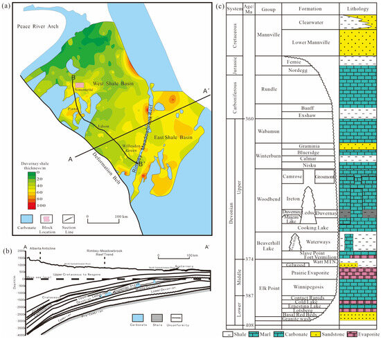
Figure 1.
Geological sketch of the Western Canada Basin [28]: (a) isopach map of the Duvernay shale (according to Lyster et al. [29]); (b) stratigraphic section (according to Price et al. [30]); (c) stratigraphic column (according to Porter et al. [31]).
Influenced by multiple tectonic activities, the WCSB exhibits a complete stratigraphic development, ranging from the Cambrian to the Quaternary. Based on different tectonic and sedimentary backgrounds, the stratigraphic system can be divided into those deposited during the craton platform period and the foreland basin period. The strata of the basin are further categorized into four major sedimentary series through four regional disconformities: Cambrian–Silurian, Devonian, Mississippian–Lower Jurassic, and Middle Jurassic–Paleogene.
In terms of sedimentary characteristics, the strata from the Cambrian to the Lower Jurassic represent stable craton shelf-margin marine and nearshore deposits formed by slow subsidence. The Middle Jurassic and Paleogene strata mainly consist of thick marine deposits, as well as non-marine foreland deposits in the eastern part of the orogenic belt. The Duvernay shale, a dark brown or black shale rich in organic matter, was formed during the maximum marine transgression event of the Woodbend Group in the Upper Devonian. It is one of the most significant source rocks in the WCSB. The stratum above the Duvernay is the Ireton Formation, while below are the strata of Majeau Lake and Beaverhill Lake limestones. The Duvernay shale covers an area of 2.43 × 10⁴ km2, with a landform of low southwest and high northeast, and a shale burial depth of 500–5500 m [30,31,32,33,34]. The Duvernay shale can be subdivided vertically into an upper shale section, a central carbonate section, and a lower shale section (Figure 2).

Figure 2.
Stratigraphic correlation of the northwest–southeast project in the Duvernay Formation in the Western Canada Basin (modified by Kong Xiangwen et al. [28]; see Figure 1a for specific section locations).
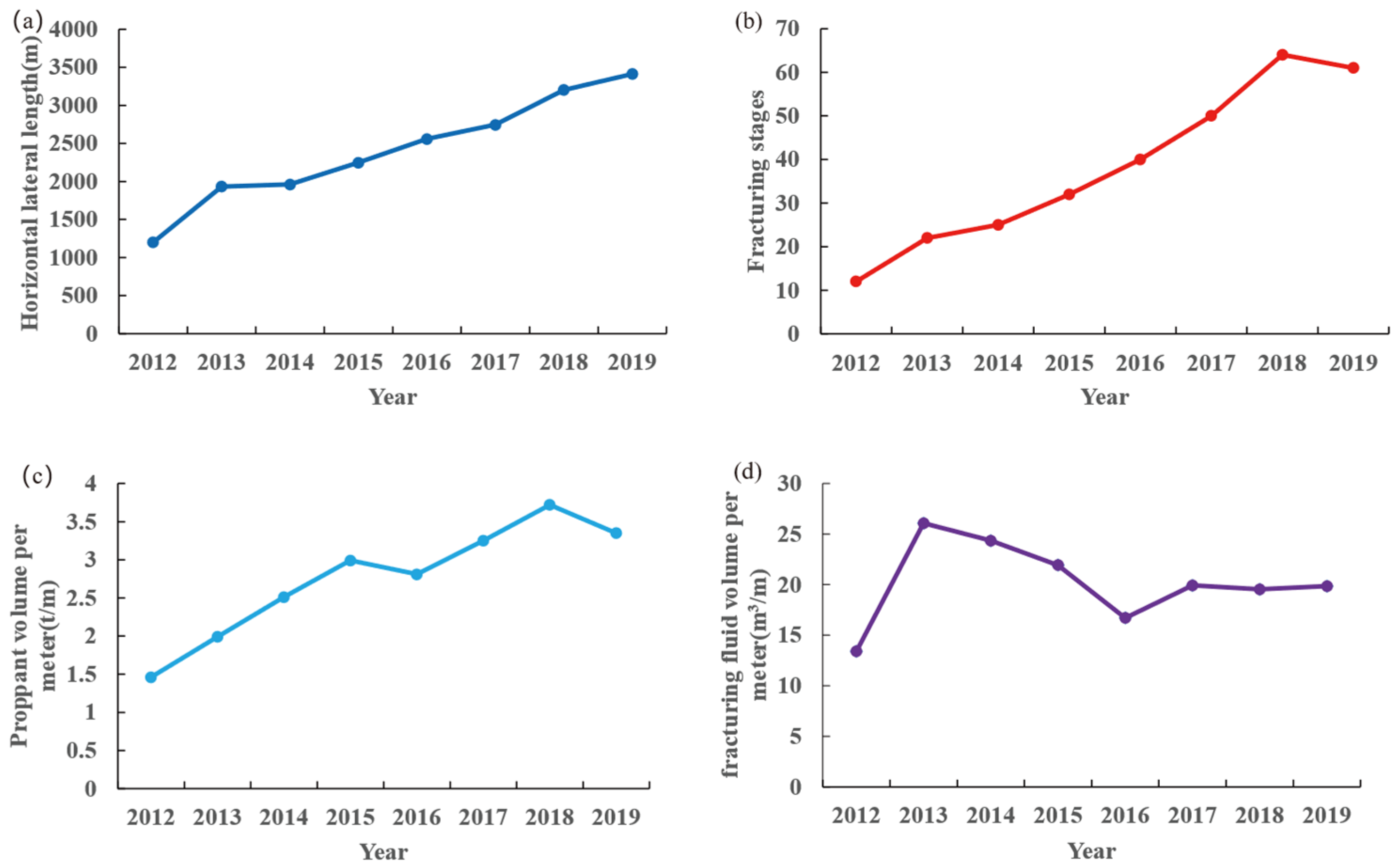
Currently, the main development block in the study area is the Simonette block with 173 production wells. Through the continuous optimization of engineering parameters since 2012, the horizontal lateral length increased from 1200 m in 2012 to 3413 m in 2019 (Figure 3a). The number of fracturing stages increased from 12 sections in 2012 to 61 sections in 2019, and the number of fracturing clusters increased from three clusters per section in 2012 to seven clusters per section in 2019. The stage and cluster spacing had been decreasing year-by-year, proppant volume per meter increased from 13.41 t/m in 2012 to 19.85 t/m in 2019, and fracturing fluid volume per meter increased significantly between 2012 and 2013, then decreased significantly and has remained unchanged at 20 m3/m (Figure 3) since 2016.
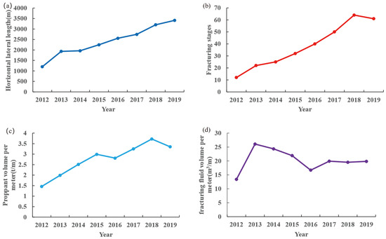
Figure 3.
Trend of fracturing parameters in the study area over the years: (a) horizontal lateral length; (b) number of fracturing stages; (c) average proppant volume; (d) average fracturing fluid volume.
The Simonette block has accumulated a large amount of geological, engineering, and production data since it was put into production in 2012. Geological data include thickness, porosity, permeability, water saturation, TOC, oil-to-gas ratio; and the engineering data include total fracturing fluid volume, total proppant volume, total clusters, total stages, horizontal lateral length, fracturing fluid type, and well spacing. Geological parameters determine the scale of the buried hydrocarbon deposited in the area, and engineering parameters determine the oil and gas production. Analyzing the existing geo-engineering data, effectively predicting “sweet spots”, and defining the parameters for well location deployment and shale engineering modifications are the key to the efficient development of this project, and machine learning provides a way of thinking about and exploring methods for mining information from the data.
3. Research Approach and Technology Roadmap
3.1. Technology Roadmap
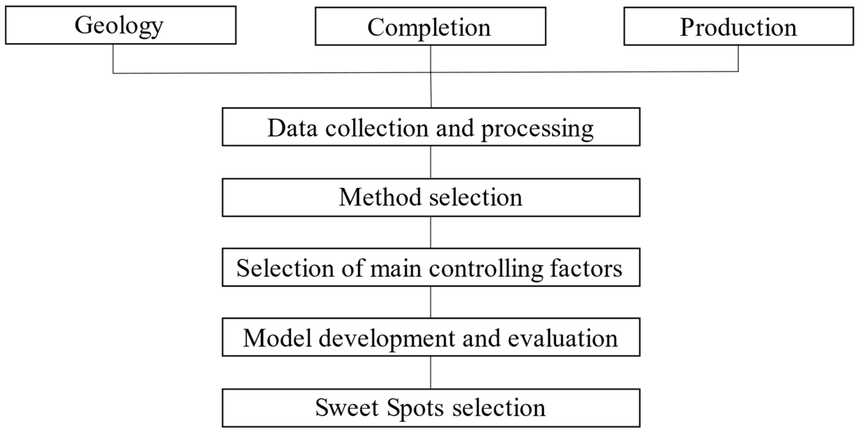
This study was conducted in five steps (Figure 4). First, the geological, engineering, and production data of the study area were collected and preprocessed; thereafter, the main controlling factors were selected; three machine learning methods were used to build a prediction model; the determination coefficient R2 and root mean square error (RMSE) were used as criteria to continuously improve the model; and finally, the model was used to select sweet spots.
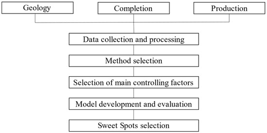
Figure 4.
Technology roadmap.
3.2. Random Forest
Random forest (RF) is an ensemble learning method proposed by Breiman [35], which is based on a bootstrap resampling technique that randomly reselects k samples as new training samples, and grows a series of decision trees based on the sample set. The final prediction result of a RF is the average of the results of all decision trees. Compared with other machine learning algorithms such as neural network, this method has various advantages such as high noise immunity, computing speed, and stability [36,37].
The basic flow of the RF algorithm is as follows.
(i) First, randomly select m samples from the data set E through bootstrap sampling to create T sub-datasets.
(ii) Use the sub-datasets to train the regression trees. During this training process, t attributes are first selected randomly for each node of a regression tree, and then the optimal cut-point is found among these t attributes.
(iii) Multiple regression tree models can be obtained by the second step, and the prediction result of each regression tree is the average of the leaf nodes where that sample is located, and the final result of the RF is the average of the prediction results of all regression trees.
3.3. Support Vector Machine
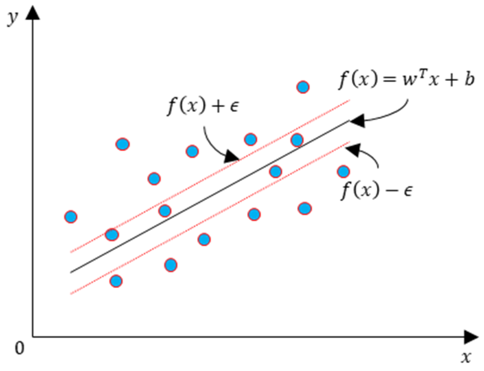
The concept of support vector machine (SVM) regression was first proposed by Vladimir Vapnik [38] in 1992, and the model can be regarded as a non-parametric model due to the existence of kernel functions. For training samples (x,y), traditional statistical models calculate the loss based on the difference between the model output value and the true value; the loss is zero when the model output value is the same as the true value. SVM regression is different in that it assumes that the tolerance of the deviation between the model output value f(x) and the true value y is at most ε, the loss is calculated when the deviation between the two value is greater than ε (Figure 5), so that the SVM problem can be expressed as:
where C is the penalty term; and are the relaxation variables; and ε is the insensitive parameter.
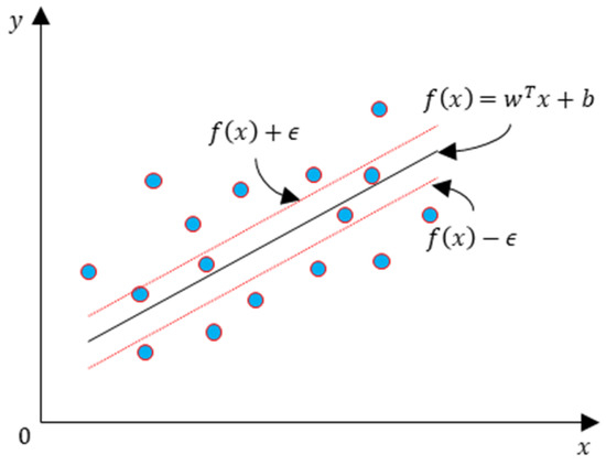
Figure 5.
Schematic diagram of support vector machine regression.
To make it easy to solve, the problem can be transformed into a dual problem using a Lagrange function, i.e.,
The corresponding parameters are obtained by the sequence minimum optimization algorithm, the block algorithm, and other methods. The kernel function is considered, and the final hyperplane equation is as follows:
where is the kernel function, which can map the sample from the original space to a high-dimensional space, making the sample linearly separable in the feature space; and and are the Lagrange multiplier vectors.
3.4. Artificial Neural Networks
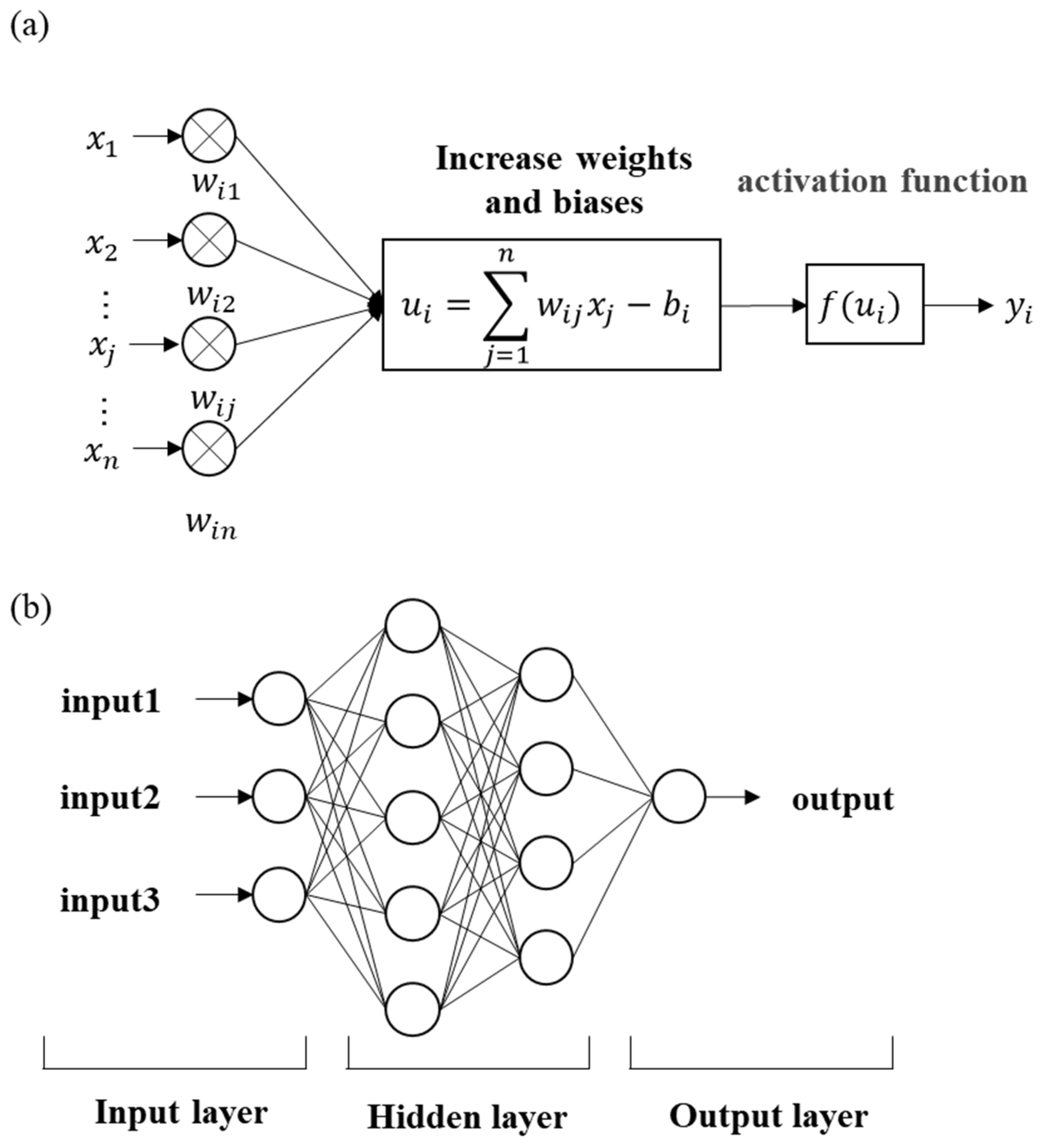
Artificial neural networks (ANN) are a widely used machine learning model that simulates the behavioral characteristics of animal neural networks to establish the relationship between data input and output [39]. Neural networks have strong associative power, strong adaptability, and strong self-organization ability, so they are widely used to solve problems such as data classification, image recognition, and nonlinear regression. The most basic component of a neural network is neurons, as shown in Figure 6a, each neuron contains weights, activation functions, and biases. In this model, neurons receive input signals from other neurons, these signals are transmitted through weighted connections, the current neuron compares the total input received with the bias of the neuron, and finally the final output of the neuron is obtained through activation function processing. The computational process for each neuron can be represented by the following formula:
where wij represents the weight between the jth neuron in the previous layer and the ith neuron in the layer; bi represents the bias of the ith neuron in the layer; xj denotes the output of the jth neuron in the previous layer; yi indicates the output of the ith neuron in the layer; f represents the activation function; and n means the number of neurons in the previous layer.
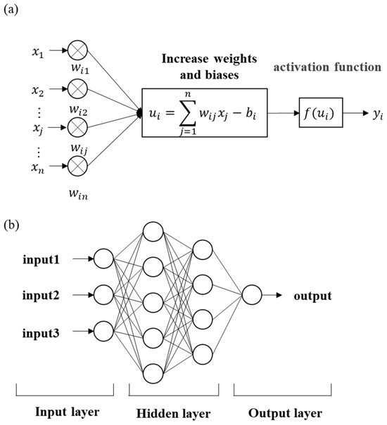
Figure 6.
Schematic diagram of the neural network model: (a) a multi-layer perceptron; (b) the calculation process of a neuron.
The training process of a neural network is to continuously adjust the weights and biases through the inputs and outputs in order to minimize the error. In this process, according to the different signals received by neurons, it can be divided into a feedforward neural network and a feedback neural network. In a feedforward neural network, the information in the entire network is propagated in one direction, and there is no back-information propagation; in a feedback neural network, neurons can receive information from other neurons as well as their own feedback signals. Due to the strong power of neural networks, some overfitting problems often occur in the actual application process, that is, the error of the training set continues to decrease, but the error of the test set may continue to increase. The usual solution is “early stop”. This method divides the dataset into a training set and a validation set, where the training set is used to calculate the gradient, bias, and weight, and the validation set is used to calculate the error. If the error of the training set decreases and the error of the validation set increases, the training is stopped and the weight and bias are obtained with the smallest verification set error.
3.5. Data Preprocessing
For oil and gas data, the magnitudes of different variables differ, and the value ranges of different attributes differ significantly, which may lead to problems when algorithms such as gradient descent are used in the model. Therefore, we used z-score standardized data (as shown in Equations (8)–(10)) in this study. After standardization, data can be converted into normally distributed data with a mean of 0 and a standard deviation of 1 to improve the data comparability.
where μ, σ, and xi are the mean, standard deviation, and normalized value of the data.
In this study, we used the One-Hot Encoding method to encode discrete attributes such as the fracturing fluid type. This method can extend the value of a discrete attribute to the Euclidean space. A value in the discrete space corresponds to a point in the Euclidean space, and the One-Hot Encoding method makes the calculation of the distance between attributes more sensible.
3.6. Model Selection and Evaluation
The RMSE and determination coefficient R2 were used as the evaluation criteria. The RMSE is the square root of the ratio of the sum of the squares of the deviation between the predicted value and the true value to the number of samples m, namely,
The determination coefficient R2 is the ratio of the regression sum of squares to the total sum of squares, namely,
where y represents true value; denotes predicted value; and is the mean value of the data.
The RMSE is a measure of the deviation between the predicted value and the true value. In general, the smaller the RMSE, the higher the accuracy of the model. The determination coefficient R2 reflects the goodness of fit of the model, and its value is between 0 and 1. The closer the value of R2 is to 1, the higher the reliability of the model.
4. Data Integration and Analysis
The geological, engineering, and production data of 173 wells were collected in this study. The wells were gathered from the same shale gas reservoir, namely Simonette. Geological and engineering data were selected as the attribute values, and the one-year cumulative oil and gas production was used as the target value. The geological data include thickness, porosity, permeability, water saturation, TOC, oil-to-gas ratio (OGR); and the engineering data include total fracturing fluid volume, total proppant volume, total clusters, total stages, horizontal lateral length, fracturing fluid type, and well spacing. In this study, the 3-Sigma Rule was applied to detect outliers. After outlier detection, 165 samples existed in the dataset. The data distribution of the variables is shown in Table 1 and Table 2.

Table 1.
Data distribution of the geological variables.

Table 2.
Data distribution of the engineering variables.
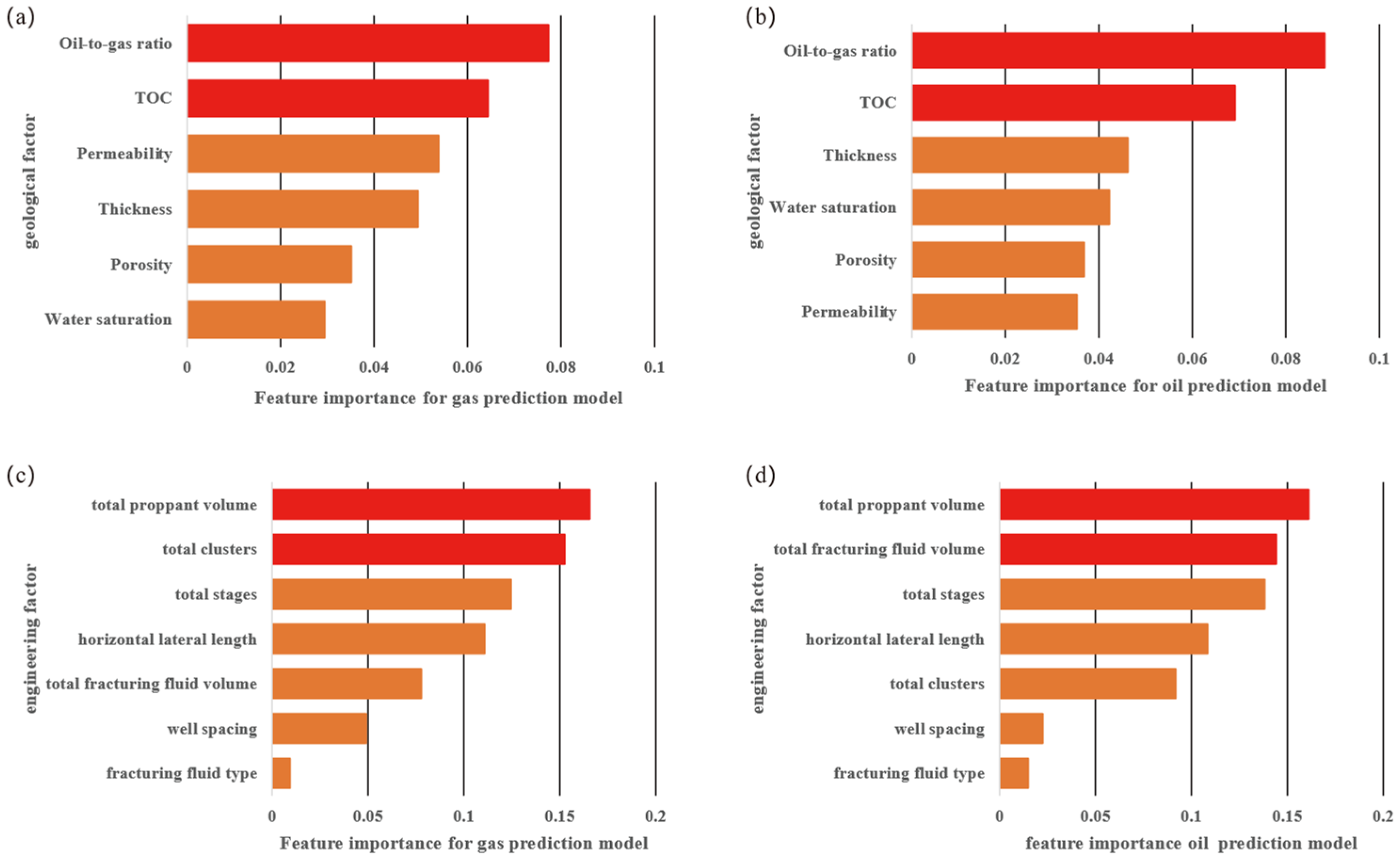
Shale oil and gas reservoirs are self-generated and self-stored reservoirs, and the geological conditions of shale formation directly determine the resource quality and scale of shale oil and gas, while engineering parameters have a great impact on the recoverability of shale oil and gas. The RF algorithm can be used to obtain the attribute importance ranking for the one-year cumulative oil and gas production (Figure 7), which can be used to analyze the main controlling factors of the oil and gas production, and serve as a reference for subsequent sweet spot selection.

Figure 7.
Ranking of geological–engineering main controlling factors: (a) feature importance ranking of geological factors for the one-year cumulative gas production prediction model; (b) feature importance ranking of geological factors for the one-year cumulative oil production prediction model; (c) feature importance ranking of engineering factors for the one-year cumulative gas production prediction model; (d) feature importance ranking of engineering factors for the one-year cumulative oil production prediction model.
4.1. Analysis of Geological Main Controlling Factors
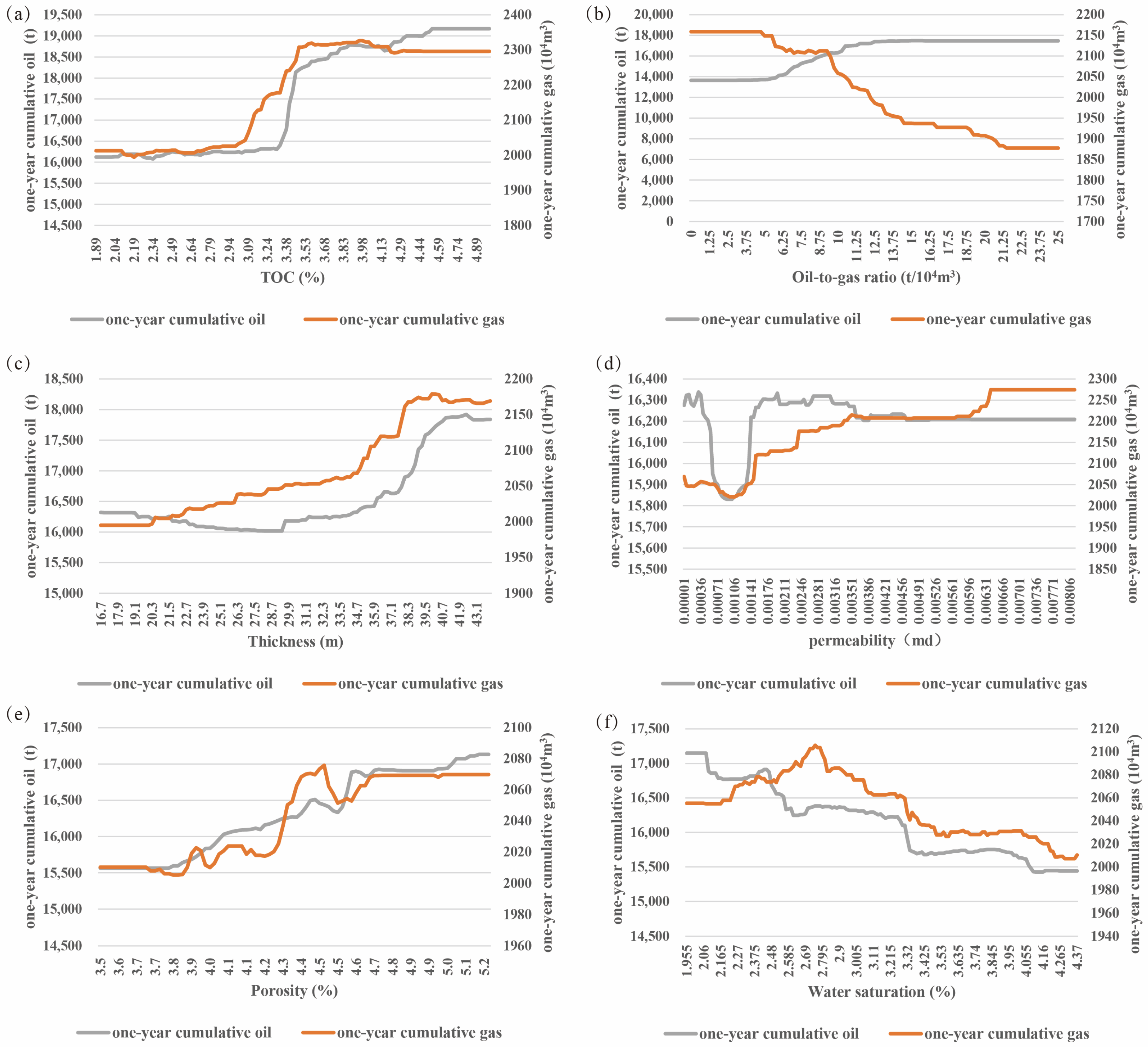
By analyzing the importance of geological factors based on machine learning, it can be concluded that two geological factors, i.e., oil-to-gas ratio and TOC, were the top two factors (Figure 7a,b), followed by four factors, i.e., permeability, effective thickness, porosity, and water saturation, indicating that the impact of the oil-to-gas ratio and TOC on the production is much greater than that of the other four factors. In the following sections, the impact of each individual geological factor on the production will be analyzed based on the shale oil/gas formation mechanism (Figure 8).
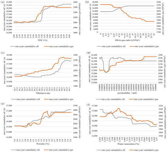
Figure 8.
Geological main controlling factors and one-year cumulative oil and gas production: (a) TOC; (b) oil-to-gas ratio; (c) thickness; (d) permeability; (e) porosity; (f) water saturation.
(1) TOC: Total organic carbon (TOC) is an important indicator of organic carbon abundance [40,41], which reflects the hydrocarbon generation capacity of the shale formation, directly determines the scale of the generated shale oil and gas, indirectly affects the sizes of organic matter pores, and also has an obvious controlling effect on the adsorbed gas in shale. The natural gas in shale will first be adsorbed in the adsorbed state on the surface of organic matter as well as rock particles, and as the adsorbed and dissolved gas saturate, the remaining gas will be transported and stored in a free state in pores or fractures. The TOC is calculated based on the resistivity and acoustic transit time logging curves using the ΔLgR technique [42]. As shown in Figure 8a, the TOC is highly positively correlated with the one-year cumulative oil and gas production.
(2) Oil-to-gas ratio: The oil-to-gas ratio indicates the amount of natural gas accompanying each ton of produced condensate oil. Since the oil-to-gas ratio is positively correlated with the shale organic matter maturity [43], its impact also reflects the controlling effect of the organic matter maturity on the production. In areas where the oil-to-gas ratio data are lacking, the organic matter maturity can be used as a substitute for this parameter. The pressure coefficient of the formation in the study area is 1.7–2.0, and the temperature gradient is 3.1 °C/100 m–3.7 °C/100 m. When the reservoir pressure exceeds the dew point pressure at its corresponding temperature and the reservoir temperature is between the critical and critical condensation temperature, the liquid hydrocarbon is back-dissolved into the gaseous hydrocarbon to form a condensate gas reservoir, and the oil and gas are mainly liquid-rich hydrocarbon. As shown in Figure 8b, the oil-to-gas ratio is negatively correlated with the one-year cumulative gas production and positively correlated with the one-year cumulative oil production.
(3) Thickness: For a commercial shale oil and gas reservoir to be formed, organic-rich shale must reach a certain thickness to ensure a sufficient scale of shale oil and gas resources. Generally speaking, high quality shale refers to organic-rich shale with a TOC level greater than 2% [44]. Shale thickness and oil and gas production are generally positively correlated, and the one-year cumulative oil and gas production gradually increases with thickness (Figure 8c).
(4) Porosity and permeability: For unconventional oil and gas, rock pores are an important space for storing oil and gas. According to the statistics, more than 50% of shale oil and gas is stored in shale pores which are of various types, e.g., intergranular, intragranular, and organic matter pores [45]. The organic matter pores can form a three-dimensional connected organic matter mesh, which can improve the pore connectivity to a certain extent. Generally speaking, the correlation of porosity is highly positive with the permeability. The porosity is calculated using the neutron-density cross plot, and the permeability is measured by building a permeability interpretation model through analysis of the porosity–permeability relationship based on cores. The one-year cumulative oil production has a good positive correlation with porosity and a poor correlation with the permeability (Figure 8d,e), which indicates that shale oil is mainly stored in shale pores in free state, and therefore the porosity of organic matter has a great impact on the shale oil production. Shale gas is stored in shale in a free state and an absorbed state, and the one-year cumulative gas production has a positive correlation with the porosity and permeability. In addition, due to the heterogeneous permeability of shale, the test sample points may not fully represent the true permeability of the production formation. Moreover, for low-permeability shale, the error of the permeability test result is high, which together cause a poorer correlation between the permeability and production than that between the porosity and production.
(5) Water saturation: Generally speaking, the lower the water saturation, the higher the hydrocarbon content in the shale reservoir space, and the more favorable to shale oil and gas development. The one-year cumulative oil and gas production is highly negatively correlated with the water saturation (Figure 8f).
4.2. Analysis of Engineering Main Controlling Factors
Among all engineering factors, the total proppant volume is the top factor that has the greatest impact on the one-year cumulative oil production and one-year cumulative gas production (Figure 7c,d). It is the most important factor affecting the one-year cumulative oil and gas production, which has been mentioned frequently in many previous papers [46,47]. Other engineering parameters, e.g., total fracturing fluid volume and fracturing fluid type, seem to be less important due to strong correlations between engineering parameters. When the total proppant volume is present in a model, other engineering parameters such as total fracturing fluid volume and cluster spacing will also be present in it.
5. Discussion
Considering the limited representativeness of the permeability and water saturation data, and the difficulty of obtaining them, these two parameters were removed from the sweet spot prediction, and the remaining eleven parameters were used to build one-year cumulative oil and gas production prediction models, namely, total fracturing fluid volume, total proppant volume, horizontal lateral length, total clusters, total stages, fracturing fluid type, well spacing, TOC, oil-to-gas ratio, thickness, and porosity.
In this study, the scikit-learn library in python 3.9 was used to build the machine learning models, and to prevent overfitting, this study used 5-fold cross-validation to separate the test set from the training set, i.e., the ratio of the number of wells in the training set to that in the test set was 4:1 (132:33). For various hyperparameters required by the model, firstly, we determined the value ranges of the hyperparameters through random searches, and then determined their specific values through grid searches.
After optimization, the hyperparameters of RF, SVM, and ANN are demonstrated in Table 3, Table 4, Table 5, Table 6 and Table 7 which illustrate the model performance for one-year cumulative gas production and one-year cumulative oil production, respectively. The model results for the training set and testing set are demonstrated in Figure 9. As for the one-year cumulative gas production prediction, the root mean squared errors (RMSE) in the testing set are found to be 460.6 × 10⁴ m3 for SVM, 487.94 × 10⁴ m3 for ANN, and 404.68 × 10⁴ m3 for RF. The RF model demonstrates the highest R2 and the lowest RMSE in both the training set and testing set. In particular, in the testing set, the RF model shows R2 at 0.82 and RMSE at 404.68 × 10⁴ m3. This indicates that the model is able to explain 82% of the gas production variance in the study area.

Table 3.
Distributions of random forest (RF) hyperparameters.

Table 4.
Distributions of support vector machine (SVM) hyperparameters.

Table 5.
Distributions of ANN hyperparameters.

Table 6.
Model results for one-year cumulative gas production.

Table 7.
Model results for one-year cumulative oil production.

Figure 9.
Comparison of prediction performance of the GPR, SVR, and MLR algorithms: (a) one-year cumulative gas production prediction model; (b) one-year cumulative oil production prediction model.
As for the one-year cumulative oil production prediction, the result is the same as the one-year cumulative gas production prediction, the R2 of the testing set is 0.67 for SVM, 0.71 for ANN, and 0.79 for RF. The RF model shows the highest R2 at 0.79 and the lowest RMSE at 3300.58t in the testing set; this also means that the RF model can illustrate 79% of the oil production variance in Duvernay shale gas reserve.
In most machine learning-based models, the R2 value has varied from 0.5 to 0.8 (Luo et al. [21], Kong et al. [48], Wang et al. [49]). The RF models applied in this study are able to provide relatively high accuracy and robustness for production prediction. Compared with SVM and ANN, RF has better performance for the prediction of one-year cumulative gas production and one-year cumulative oil production. Therefore, the RF method was selected to apply sweet spot prediction.
6. Results
The one-year cumulative oil production model and one-year cumulative gas production prediction model contain two types of parameters, i.e., geological and engineering parameters. Geological parameters determine the scale and quality of the resources, and engineering parameters affect the resource recoverability. We can input predicted geological parameters and generalized engineering parameters into the models to analyze the abundance of recoverable reserves in some sparsely drilled areas, and thereby provide a basis for future well location deployment and assessment of recoverable reserves in these areas.
The planar distributions of geological parameters such as TOC, oil-to-gas ratio, thickness, and porosity in the study area are shown in Figure 10. As shown in the distribution of thickness, the shale thickness in the study area gradually increases from northwest to southeast, and the thickness in some southern parts of the area can reach 50 m. The planar distribution of TOC is based on well-to-well interpolation, and the TOC of each well is calculated based on the resistivity and acoustic transit-time logging curves. As shown in the planar distribution of TOC, the TOC values in the west and south of the study area are high, and even higher than 5% in some parts of the area. The planar distribution of the oil-to-gas ratio is also based on well-to-well interpolation, or organic matter maturity. It gradually decreases from northwest to southeast, and is close to 0 in some southern parts of the area (Figure 10).

Figure 10.
Planar distributions of geological parameters: (a) thickness; (b) TOC; (c) oil-to-gas ratio; (d) porosity.
Engineering parameters can usually be optimized with the progress of technologies. Different values of engineering parameters can cause different distributions of recoverable reserves. Since 2012, the horizontal lateral length and number of stages have grown year-by-year and the stage spacing has decreased year-by-year. Since 2016, the number of clusters per section has risen considerably and the total proppant volume per meter has increased year-by-year. The fracturing fluid volume per meter increased significantly between 2012 and 2013, then dropped significantly, and has remained unchanged at 20 m3/m (Figure 3) since 2016. The average values of the engineering parameters in 2013, 2015, 2017, and 2018 were selected as the engineering parameter inputs for schemes 1, 2, 3, and 4, respectively, and the specific input values of the engineering parameters for the four schemes are listed in Table 8 below.

Table 8.
Engineering parameters used in different schemes.
The values of engineering parameters and geological parameters are input into the one-year cumulative oil production model and one-year cumulative gas production prediction model to obtain a series of predicted values. Since the one-year cumulative gas production is well correlated with the estimated ultimate recovery (EUR) of gas per well, and the one-year cumulative oil production is well correlated with the EUR of oil per well (Figure 11), the following equations can be used to calculate the EUR of oil and EUR of gas.
Gas − EUR = 3.5055 × one-year cumulative gas
Oil − EUR = 2.596 × one-year cumulative oil

Figure 11.
(a) One-year cumulative gas production vs. gas EUR. (b) One-year cumulative oil production vs. oil EUR.
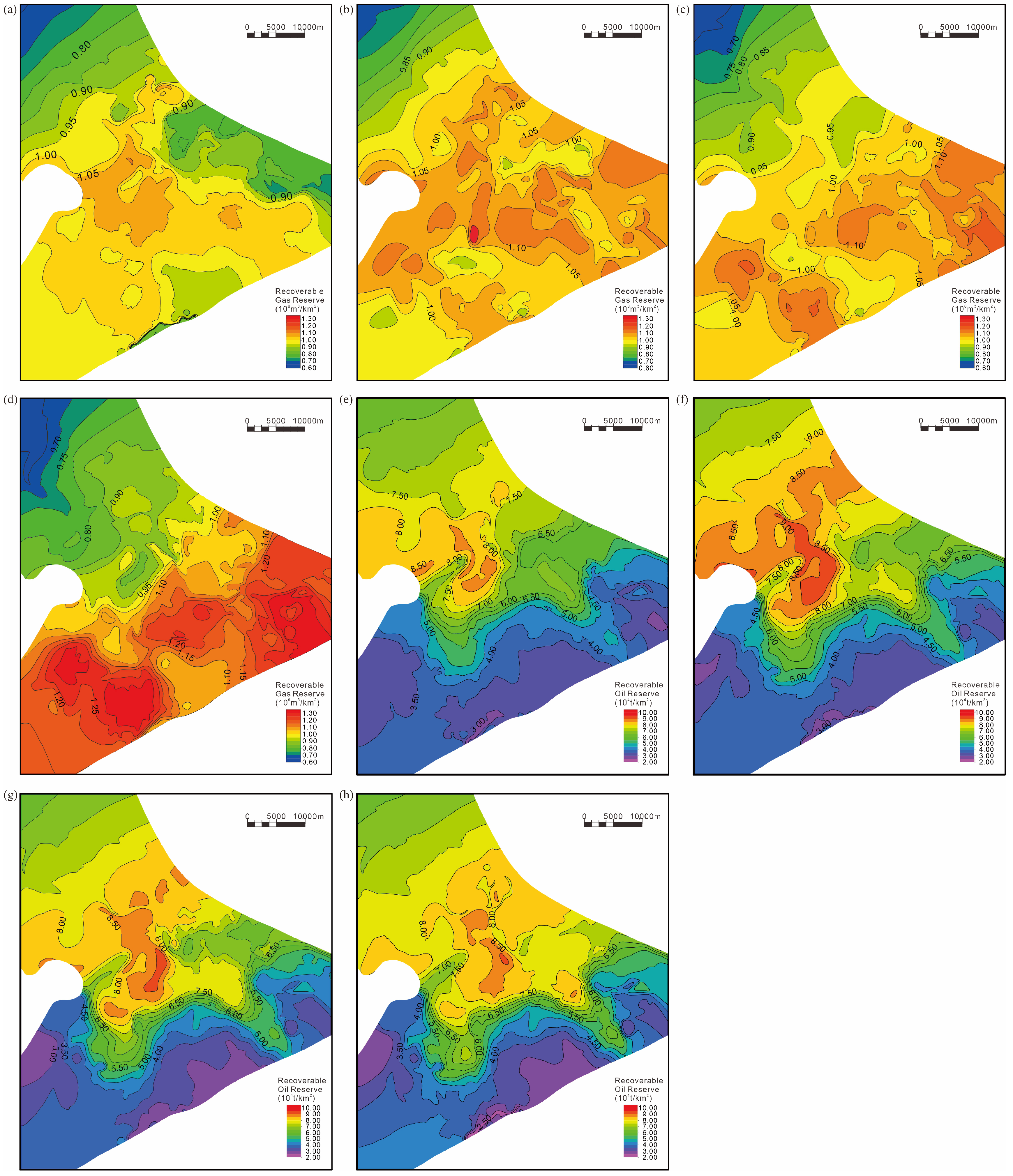
The horizontal lateral length input in the model is 3000 m; the well spacing is usually 300 m; and the well-controlled area of each well is 0.9 km2. We can obtain the predicted EUR values of oil and gas and the abundance of recoverable reserves per unit area based on the normalized well-controlled area. The distributions of abundance of recoverable reserves resulting from different schemes are shown in Figure 12.
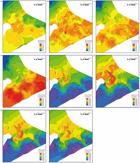
Figure 12.
Distributions of abundance of recoverable reserves: (a) gas-scheme 1; (b) gas-scheme 2; (c) gas-scheme 3; (d) gas-scheme 4; (e) oil-scheme 1; (f) oil-scheme 2; (g) oil-scheme 3; (h) oil-scheme 4.
According to the analysis results, the distribution patterns of recoverable gas reserves resulting from all the schemes are consistent with one another, namely, gradually increasing from northwest to southeast (Figure 12a–d), as is the case with the oil-to-gas ratio. The scales of recoverable gas reserves resulting from different schemes differ from one another. From scheme 1 to scheme 4, the engineering parameters such as total fracturing fluid volume, total proppant volume, and total clusters gradually increase, and so does the scale of recoverable gas reserves. The recoverable gas reserves in some parts of scheme 4 can reach 1.34 × 10⁸ m3/km2, indicating that the more aggressive the scheme, the higher the gas production.
The distribution patterns of recoverable shale oil reserves resulting from all the schemes are consistent with one another, with lower values in the southwestern and northeastern parts of the area and higher values in the central part of the area (Figure 12e–h). Their distribution patterns differ from those of the oil-to-gas ratio, and are close to zero in the southeastern and southern parts of the area. In the abundance graph of recoverable oil reserves, values in these parts are low as well. The shale in the northern part has a low TOC, thin thickness, and limited total organic hydrocarbon. The scales of recoverable oil reserves resulting from different schemes differ from one another. From scheme 1 to scheme 4, the engineering parameters such as total fracturing fluid volume, total proppant volume, and total clusters gradually increase, and so does the scale of recoverable oil reserves. As shown in Figure 12e–h, the parts with an abundance of recoverable reserves higher than 8 × 10⁴ t/km2 are expanding, also indicating that the more aggressive the scheme, the higher the oil production. However, the abundance of recoverable reserves in the central part of the study area resulting from scheme 2 is higher than those resulting from the more aggressive schemes 3 and 4, which indicates that the production is not directly linearly correlated with the engineering parameters, and a more appropriate scheme may cause a higher production under certain geological conditions, which requires further studies.
This study is based on the utilization of several machine learning techniques for predicting shale oil and gas reserves and obtaining good results. It is important to note that while the model used in this study may provide some suggestions for sweet spot prediction in the Duvernay Formation, it is not applicable to use the same model in a completely different shale gas reserve. Furthermore, the machine learning model does not take parent and child well interference into consideration, which may limit the prediction accuracy of sweet spots.
7. Conclusions
Herein, we built recoverable gas and recoverable oil reserve prediction models using three machine learning methods as well as the geological, engineering, and production data of the Duvernay shale oil and gas field in the Western Canada Basin. The R2 values of the prediction models were 0.7894 and 0.8210, respectively. The results intuitively reflect the impacts of different geological and engineering factors on the recoverable oil and gas reserves, reliably predict the distributions of recoverable shale oil and gas reserves, and provide a basis for future well location deployment.
The main geological factors on the recoverable reserves of the Duvernay shale oil and gas field are shale maturity and TOC. The thickness of organic-rich shale and water saturation have a greater impact on the recoverable shale oil reserves, while the physical properties of shale have a greater impact on the recoverable gas reserves. The differences in the controlling factors between the two are mainly caused by the different oil and gas enrichment mechanisms in shale reservoirs. The main engineering factor affecting the recoverable oil and gas reserves in Duvernay is the total proppant volume. The total fracturing fluid volume has a greater impact on the recoverable shale oil reserves, while the total clusters have a greater impact on the recoverable shale-gas reserves, followed by other engineering factors such as the total stages and horizontal lateral length.
Under the control of geological factors such as shale maturity, thickness of organic-rich shale, and TOC, the abundance of recoverable shale-gas reserves is high and the abundance of recoverable oil reserves is low in the southeastern part of the study area; the abundance of recoverable oil and gas reserves is low in the northern part of the study area; the abundance of recoverable shale oil and gas reserves is relatively high in the central part of the study area due to a moderate shale maturity, high TOC, and high thickness of organic-rich shale, and therefore the central part of the study area is a shale oil and gas sweet spot for future well location deployment.
Author Contributions
Data curation, Y.S. and P.W.; supervision, H.W. and X.Z.; validation, X.K.; writing—review and editing, Z.G. All authors have read and agreed to the published version of the manuscript.
Funding
This research was funded by Major Science and Technology Project of PetroChina, grant number 2023ZZ0703.
Institutional Review Board Statement
Not applicable.
Informed Consent Statement
Not applicable.
Data Availability Statement
Data is contained within the article.
Conflicts of Interest
The authors declare no conflicts of interest.
Nomenclature
| Abbreviation | Full Name |
| R2 | Determination coefficient |
| RMSE | Root mean square error |
| RF | Random Forest |
| EUR | Estimated Ultimate Recovery |
| TOC | Total Organic Carbon Content (%) |
References
- Wang, H.; Ma, F.; Tong, X.; Liu, Z.; Zhang, X.; Wu, Z.; Li, D.; Wang, B.; Xie, F.; Yang, L. Assessment of global unconventional oil and gas resources. Pet. Explor. Dev. 2016, 43, 925–940. [Google Scholar] [CrossRef]
- Zhang, X.S.; Wang, H.J.; Ma, F.; Sun, X.C.; Zhang, Y.; Song, Z.H. Classification and characteristics of tight oil plays. Pet. Sci. 2016, 13, 18–33. [Google Scholar] [CrossRef]
- Shelley, B.; Grieser, B.; Johnson, B.J.; Fielder, E.O.; Heinze, J.R.; Werline, J.R. Data analysis of Barnett shale completions. SPE J. 2008, 13, 366–374. [Google Scholar] [CrossRef]
- Baihly, J.; Altman, R.; Aviles, I. Has the economic stage count been reached in the Bakken shale? In Proceedings of the SPE Hydrocarbon Economics and Evaluation Symposium, Calgary, AB, Canada, 24–25 September 2012. [Google Scholar]
- Lafollette, R.F.; Holcomb, W.D.; Aragon, J. Practical Data Mining: Analysis of Barnett Shale Production Results with Emphasis on Well Completion and Fracture Stimulation. In Proceedings of the SPE Hydraulic Fracturing Technology Conference, The Woodlands, TX, USA, 6–8 February 2012. [Google Scholar]
- Shelley, R.; Guliyev, N.; Nejad, A. A Novel Method to Optimize Horizontal Bakken Completions in a Factory Mode Development Program. In Proceedings of the SPE Annual Technical Conference and Exhibition, San Antonio, TX, USA, 8–10 October 2012. [Google Scholar]
- Pearson, C.M.; Griffin, L.; Wright, C.; Weijers, L. Breaking Up is Hard to Do: Creating Hydraulic Fracture Complexity in the Bakken Central Basin. In Proceedings of the SPE Hydraulic Fracturing Technology Conference, The Woodlands, TX, USA, 5 February 2013; p. D021S006R005. [Google Scholar]
- Newgord, C.; Mediani, M.; Ouenes, A.; O’Conor, P. Predicting Middle Bakken Well Performance with Shale Capacity. In Proceedings of the SPE Annual Technical Conference and Exhibition, Houston, TX, USA, 28–30 September 2015; p. D011S001R003. [Google Scholar]
- Schuetter, J.; Mishra, S.; Zhong, M.; LaFollette, R. Data Analytics for Production Optimization in Unconventional Reservoirs. In Proceedings of the SPE/AAPG/SEG Unconventional Resources Technology Conference, San Antonio, TX, USA, 20–22 July 2015. [Google Scholar]
- Lolon, E.; Hamidieh, K.; Weijers, L.; Mayerhofer, M.; Melcher, H.; Oduba, O. Evaluating the Relationship between Well Parameters and Production Using Multivariate Statistical Models: A Middle Bakken and Three Forks Case History. In Proceedings of the SPE Hydraulic Fracturing Technology Conference, The Woodlands, TX, USA, 9–11 February 2016; p. D031S007R003. [Google Scholar]
- Wang, S.; Chen, S. A Comprehensive Evaluation of Well Completion and Production Performance in Bakken Shale Using Data-Driven Approaches. In Proceedings of the SPE Asia Pacific Hydraulic Fracturing Conference, Beijing, China, 24–26 August 2016; p. D011S002R005. [Google Scholar]
- Mohaghegh, S.D.; Gaskari, R.; Maysami, M. Shale Analytics: Making Production and Operational Decisions Based on Facts: A Case Study in Marcellus Shale. In Proceedings of the SPE Hydraulic Fracturing Technology Conference and Exhibition, The Woodlands, TX, USA, 24–26 January 2017; p. D031S007R004. [Google Scholar]
- Tian, Y.; Ayers, W.B.; Sang, H.; McCain, W.D., Jr.; Ehlig-Economides, C. Quantitative Evaluation of Key Geological Controls on Regional Eagle Ford Shale Production Using Spatial Statistics. SPE Reserv. Eval. Eng. 2018, 21, 238–256. [Google Scholar] [CrossRef]
- He, Q.; Bruno, J.; Zhong, Z. Controlling Factors of Shale Gas Production: What Can Artificial Intelligence Tell Us? In Proceedings of the SPE Eastern Regional Meeting, Charleston, WV, USA, 16 October 2019; p. D021S002R004. [Google Scholar]
- Ahmed, A.A.; Elkatatny, S.; Abdulraheem, A.; Mahmoud, M. Application of artificial intelligence techniques in estimating oil recovery factor for water derive sandy reservoirs. In Proceedings of the SPE Kuwait Oil and Gas Show and Conference, Mishref, Kuwait, 2–5 October 2017. [Google Scholar]
- Mahmoud, A.A.; Elkatatny, S.; Chen, W.; Abdulraheem, A. Estimation of oil recovery factor for water drive sandy reservoirs through applications of artificial intelligence. Energies 2019, 12, 3671. [Google Scholar] [CrossRef]
- Qin, Z.; Xu, T. Shale gas geological “sweet spot” parameter prediction method and its application based on convolutional neural network. Sci. Rep. 2022, 12, 15405. [Google Scholar] [CrossRef] [PubMed]
- Zhai, G.; Li, J.; Jiao, Y.; Wang, Y.; Liu, G.; Xu, Q.; Wang, C.; Chen, R.; Guo, X. Applications of chemostratigraphy in a characterization of shale gas Sedimentary Microfacies and predictions of sweet spots—Taking the Cambrian black shales in Western Hubei as an example. Mar. Pet. Geol. 2019, 109, 547–560. [Google Scholar] [CrossRef]
- Jiachen, H. Production Forecast Modeling and Application Based on Machine Learning. Ph.D. Thesis, China University of Geosciences, Beijing, China, 2020. [Google Scholar]
- Song, X.; Liu, Y.; Ma, J.; Wang, J.; Kong, X.; Ren, X. Productivity forecast based on support vector machine optimized by grey wolf optimizer. Lithol. Reserv. 2020, 32, 134–140. [Google Scholar]
- Luo, G.; Tian, Y.; Bychina, M.; Ehlig-Economides, C. Production-Strategy Insights Using Machine Learning: Application for Bakken Shale. SPE Reserv. Eval. Eng. 2019, 22, 800–816. [Google Scholar] [CrossRef]
- Maucec, M.; Garni, S. Application of Automated Machine Learning for Multi-Variate Prediction of Well Production. In Proceedings of the SPE Middle East Oil and Gas Show and Conference, Manama, Bahrain, 18–21 March 2019; p. D032S069R003. [Google Scholar]
- Guo, Z.; Wang, H.; Kong, X.; Shen, L.; Jia, Y. Machine Learning-Based Production Prediction Model and Its Application in Duvernay Formation. Energies 2021, 14, 5509. [Google Scholar] [CrossRef]
- Whalen, M.T.; Day, J.E. Cross-Basin Variations in Magnetic Susceptibility Influenced by Changing Sea Level, Paleogeography, and Paleoclimate: Upper Devonian, Western Canada Sedimentary Basin. J. Sediment. Res. 2010, 80, 1109–1127. [Google Scholar] [CrossRef]
- Egenhoff, S.O.; Fishman, N.S. Traces In the Dark—Sedimentary Processes and Facies Gradients In the Upper Shale Member of the Upper Devonian-Lower Mississippian Bakken Formation, Williston Basin, North Dakota, U.S.A. J. Sediment. Res. 2013, 83, 803–824. [Google Scholar] [CrossRef]
- Clarkson, C.R.; Haghshenas, B.; Ghanizadeh, A.; Qanbari, F.; Williams-Kovacs, J.D.; Riazi, N.; Debuhr, C.; Deglint, H.J. Nanopores to megafractures: Current challenges and methods for shale gas reservoir and hydraulic fracture characterization. J. Nat. Gas Sci. Eng. 2016, 31, 612–657. [Google Scholar] [CrossRef]
- Wang, P.; Chen, Z.; Jin, Z.; Jiang, C.; Sun, M.; Guo, Y.; Chen, X.; Jia, Z. Shale oil and gas resources in organic pores of the Devonian Duvernay Shale, Western Canada Sedimentary Basin based on petroleum system modeling. J. Nat. Gas Sci. Eng. 2018, 50, 33–42. [Google Scholar] [CrossRef]
- Kong, X.; Wang, P.; Xia, Z.; Zhang, X.; Qu, L.; Guo, Z. Geological characteristics and fluid distribution of the Upper Devonian Duvernay shale in Simonette block in the Western Canada Sedimentary Basin. China Pet. Explor. 2022, 27, 93–107. [Google Scholar]
- Lyster, S.; Corlett, H.; Berhane, H. Hydrocarbon Resource Potential of the Duvernay Formation in Alberta-Update; AER/AGS Open File Report 2017-02; Alberta Geological Survey/Alberta Energy Regulator: Edmonton, AB, Canada, 2017; pp. 31–43. [Google Scholar]
- Price, R. Cordilleran tectonics and the evolution of the Western Canada Sedimentary Basin. Bull. Can. Pet. Geol. 1990, 38, 176–177. [Google Scholar]
- Porter, J.; Price, R.; Mccrossan, R. The western Canada sedimentary basin. Philos. Trans. R. Soc. Lond. Ser. A Math. 1982, 305, 169–192. [Google Scholar]
- Anfort, S.; Bachu, S.; Bentley, L. Regional-scale hydrogeology of the Upper Devonian-Lower Cretaceous sedimentary succession, south-central Alberta basin, Canada. AAPG Bull. 2001, 85, 637–660. [Google Scholar]
- Green, D.G.; Mountjoy, E.W. Fault and conduit controlled burial dolomitization of the Devonian west-central Alberta Deep Basin. Bull. Can. Pet. Geol. 2005, 53, 101–129. [Google Scholar] [CrossRef]
- Li, G.; Luo, K.; Shi, D. Key technologies, engineering management and important suggestions of shale oil/gas development: Case study of a Duvernay shale project in Western Canada Sedimentary Basin. Pet. Explor. Dev. 2020, 47, 739–749. [Google Scholar] [CrossRef]
- Breiman, L. Random forests. Mach. Learn. 2001, 45, 5–32. [Google Scholar] [CrossRef]
- James, G.; Witten, D.; Hastie, T.; Tibshirani, R. An Introduction to Statistical Learning with Applications in R, 6th ed.; Springer Texts in Statistics; Springer: Berlin/Heidelberg, Germany, 2015. [Google Scholar]
- Genuer, R.; Poggi, J.M.; Tuleau-Malot, C.; Villa-Vialaneix, N. Random forests for big data. Big Data Res. 2017, 9, 28–46. [Google Scholar] [CrossRef]
- Vapnik, V. The Nature of Statistical Learning Theory; Springer: New York, NY, USA, 2000; pp. 1–15. [Google Scholar]
- Lecun, Y.; Bengio, Y.; Hinton, G. Deep learning. Nature 2015, 521, 436–444. [Google Scholar] [CrossRef]
- Zou, C.; Dong, D.; Wang, Y.; Li, X.; Huang, J.; Wang, S.; Gaun, Q.; Zhang, C.; Wang, H.; Liu, H.; et al. Shale gas in China: Characteristics, challenges and prospects (I). Pet. Explor. Dev. 2015, 42, 689–701. [Google Scholar] [CrossRef]
- Zhao, X.; Zhou, L.; Pu, X.; Jin, F.; Shi, Z.; Han, W.; Jiang, W.; Han, G.; Zhang, W.; Wang, H.; et al. Formation conditions and enrichment model of retained petroleum in lacustrine shale: A case study of the Paleogene in Huanghua depression, Bohai Bay Basin, China. Pet. Explor. Dev. 2020, 47, 856–869. [Google Scholar] [CrossRef]
- Liu, C.; Lu, S.F.; Xue, H.T. Variable-coefficient ΔlogR model and its application in shale organic evaluation. Prog. Geophys. 2014, 29, 312–317. [Google Scholar]
- Zou, C.N.; Ma, F.; Pan, S.Q. Formation and distribution potential of global shale oil and the theoretical and technological progress of continental shale oil in China. Earth Sci. Front. 2023, 30, 128–142. [Google Scholar]
- Zou, C.; Dong, D.; Wang, Y.; Li, X.; Huang, J.; Wang, S.; Guan, Q.; Zhang, C.; Wang, H.; Liu, H.; et al. Shale gas in China: Characteristics, challenges and prospects (II). Pet. Explor. Dev. 2016, 43, 166–178. [Google Scholar] [CrossRef]
- Zou, C.; Dong, D.; Wang, S.; Li, J.; Li, X.; Wang, Y.; Li, D.; Cheng, K. Geological characteristics, formation mechanism and resource potential of shale gas in China. Pet. Explor. Dev. 2010, 37, 641–653. [Google Scholar] [CrossRef]
- Liao, L.; Li, G.; Zhang, H.; Feng, J.; Zeng, Y.; Ke, K.; Wang, Z. Well Completion Optimization in Canada Tight Gas Fields Using Ensemble Machine Learning. In Proceedings of the Abu Dhabi International Petroleum Exhibition & Conference, Abu Dhabi, United Arab Emirates, 9–12 November 2020. [Google Scholar]
- Sheikhi Garjan, Y.; Ghaneezabadi, M. Machine Learning Interpretability Application to Optimize Well Completion in Montney. In Proceedings of the SPE Canada Unconventional Resources Conference, Virtual, 28 September–2 October 2020; p. D033S004R003. [Google Scholar]
- Kong, B.; Chen, Z.; Chen, S.; Qin, T. Machine learning-assisted production data analysis in liquid-rich Duvernay Formation. J. Pet. Sci. Eng. 2021, 200, 108377. [Google Scholar] [CrossRef]
- Wang, S.; Chen, S. Insights to fracture stimulation design in unconventional reservoirs based on machine learning modeling. J. Pet. Sci. Eng. 2019, 174, 682–695. [Google Scholar] [CrossRef]
Disclaimer/Publisher’s Note: The statements, opinions and data contained in all publications are solely those of the individual author(s) and contributor(s) and not of MDPI and/or the editor(s). MDPI and/or the editor(s) disclaim responsibility for any injury to people or property resulting from any ideas, methods, instructions or products referred to in the content. |
© 2024 by the authors. Licensee MDPI, Basel, Switzerland. This article is an open access article distributed under the terms and conditions of the Creative Commons Attribution (CC BY) license (https://creativecommons.org/licenses/by/4.0/).


