Prediction of Remaining Service Life of Miniature Circuit Breakers Based on Wiener Process

Abstract

In the operation of a power distribution system, miniature circuit breakers (MCBs) are subjected to the synergistic effect of electrical and mechanical stresses in service, and their operational performance is progressively degraded, which is prone to bring significant losses to the users after failures occur. In order to accurately predict the remaining electrical life of MCBs in service, MCB mechanical characterization and dynamic simulation are carried out, and the initial closing angle of MCBs is selected as the degradation characteristic quantity, so as to deeply analyze the evolutionary characteristics of the initial closing angle in the degradation of MCBs and to construct the electrical degradation model of the one-dimensional linear Wiener process in the present study. With the help of the Monte Carlo method, we carry out the electric life simulation analysis to investigate the intrinsic correlation between the degradation of electric performance and the initial closing angle, and we implement the electric life experiment under the 63 A working condition to analyze the dynamic change in the stiffening angle of the test samples. The parameters of the electrical performance degradation model are identified through the synergistic driving of the electrical life simulation data and the experimental data, the remaining electrical life prediction is realized based on the degradation data of the same batch of products, and the maximum prediction error of the proposed method is controlled within 15%.

1. Introduction

Circuit breakers, as crucial electrical equipment in power systems, can automatically cut off fault circuits and protect transmission lines and electrical devices. During their service life, the electrical stress generated by each switching operation (making and breaking) erodes the contact system. Over time, this reduces the reliability of circuit breakers, and may even cause them to lose their original functions, threatening the safe operation of a power distribution system. Therefore, it is necessary to effectively and accurately predict the remaining useful life (RUL) of circuit breakers.

Scholars at home and abroad have actively engaged in research on the remaining useful life (RUL) prediction and reliability assessment of switching appliances [1,2], selecting different characteristic signals according to the inherent characteristics of various switching appliances. In reference [3], vibration signals generated during the operation of conventional circuit breakers (CCBs) were extracted, and a remaining useful life (RUL) prediction model based on a self-attention bidirectional long short-term memory network (SA-BiLSTM) was constructed to accurately predict the remaining life of CCBs. Reference [4] conducted constant-stress accelerated degradation tests on thermal trips using temperature as the acceleration stress and specific heat deflection as the degradation characteristic quantity. The Wiener process and maximum likelihood estimation were employed to estimate RUL parameters, determine the remaining life of thermal trips under various acceleration stresses, and deduce the RUL of external thermal trips under normal stress via the Arrhenius acceleration model. Reference [5] combined statistical theory with the Arrhenius model for the life prediction of electronic residual current circuit breakers, with prediction results close to the reference service life provided by manufacturers. Reference [6] designated the residual working current as the degradation evaluation quantity for RCBOs (residual current operated breakers), established an optimized BP neural network (BPNN) model based on test degradation data, and optimized the BPNN model using a genetic algorithm. The relative error between the predicted life and the true value was less than 10%. Reference [7] addressed the impact of the common failure modes of circuit breakers on travel curves, organizing a fuzzy probability method via maximum likelihood and an interactive multiple model (IMM) to accurately predict circuit breaker states and intelligently detect failure causes. Reference [8] considered the effects of arc voltage and arc restrike in AC contactors, established a remaining electrical life prediction method based on Bayesian theory using Joule integral as the degradation indicator, and improved the accuracy of RUL prediction.

Methods for remaining useful life (RUL) prediction and reliability assessment can be primarily categorized into physics-of-failure (PoF) methods and data-driven methods. PoF methods establish mathematical degradation models and predict lifespan based on the internal failure mechanisms of test specimens. However, different types of electrical appliances exhibit distinct internal mechanisms, which are often highly complex and challenging to study comprehensively. Taking MCBs as an example, the wear and oxidation behavior of contact materials are significantly affected by factors such as manufacturing processes and environmental temperature and humidity, leading to significant differences in the failure mechanisms of different samples. In actual operation, MCBs are subject to complex and variable conditions such as overload currents, operating frequencies, and environmental vibrations, which are difficult to fully reproduce through standard laboratory testing. This results in significant errors in parameter calibration based on physical models. Data-driven methods are further divided into artificial intelligence (AI) approaches and statistical model methods. AI approaches, characterized by their robust nonlinear modeling capabilities, excel at processing large-scale data with strong adaptability. Common AI methods include neural networks [9], support vector machines [10], and gray models [11]. In Reference [12], the Savitzky–Golay convolution smoothing algorithm was applied to degrade data throughout the lifecycle of AC circuit breakers, followed by precise time-series prediction using a long short-term memory (LSTM) neural network, achieving a prediction accuracy of 97.4%. Reference [13] proposed a novel wavelet-enhanced dual-tree residual network, decomposing time-series data into high-frequency and low-frequency components via wavelet transform to predict the RUL of circuit breaker operating mechanisms. Reference [14] analyzed characteristic parameter changes in relays in salt spray environments and developed a genetic algorithm–backpropagation neural network (GA-BP) model, significantly improving state recognition accuracy. Reference [15] introduced an RUL prediction method combining gray relational analysis (GRA) and LSTM, using GRA to screen mechanical parameters (e.g., overtravel, opening distance, and synchronization) as inputs for the LSTM model to accurately predict the circuit breaker lifespan. Reference [16] uses digital image processing (DIP) technology to analyze the new three-dimensional (3D) FRA features of power transformers. The proposed new 3D features integrate the frequency, amplitude, and phase angle of traditional FRA features into a single 3D graph and are processed using DIP code to extract unique texture analysis features. These features are used to classify various faults by clustering them in a ternary graph. Despite their effectiveness, AI methods face limitations such as black-box opaqueness, poor interpretability, scenario-specific applicability, and overfitting in small-data contexts.

Statistical model methods, grounded in mathematical theory and probabilistic–statistical hypotheses, describe relationships between variables through formulas and rely on rigorous statistical inference and hypothesis testing. These methods offer strong interpretability, with model parameters possessing clear physical meanings. In scenarios with small sample sizes (e.g., hundreds of data points) or low data noise, statistical models are less prone to overfitting and can validate their effectiveness through hypothesis tests (such as t-tests and F-tests). Reference [17] selected the loss rate of the spring reaction force and impact reaction force as the degradation characteristics, obtained the degradation curves of electromagnetic releases at different temperatures via accelerated life testing, and derived full-life data during normal operation using the Arrhenius equation. Reference [18] proposed a hybrid method for circuit breaker (CB) prediction, integrating a hybrid prediction model with the concept of dynamic reliability through piecewise deterministic Markov processes and modeling uncertain failure thresholds to incorporate and propagate uncertain fault assessment levels during prediction estimation. Reference [19] introduced random effects into the Tweedie exponential dispersion process model to capture individual differences, enabling the more accurate fitting of degradation processes, and derived the service life under actual temperature and humidity conditions via the Peck acceleration model. Reference [20], based on the topological structure of hybrid DC circuit breakers, used fault tree analysis to identify basic components causing breaker failures and introduced Markov models into the reliability modeling of hybrid DC circuit breakers to calculate the steady-state availability, failure rates, and mean time between failures. Reference [21] established a degradation model based on the Wiener process, proposed the probability density function (PDF) of the remaining electrical life (REL) of AC contactors by understanding the first accumulation of contact erosion loss (CEL) exceeding the failure threshold, calculated the point and interval estimates of the REL, and conducted simulated electrical life tests using Monte Carlo methods. Reference [22], to predict the correlation between different degrees of contact degradation and dynamic resistance waveform characteristics, extracted five diagnostic parameters from dynamic resistance measurement (DRM) curves. Using scoring and weighting techniques, health indices were applied to clearly identify whether the CB’s condition was healthy, requiring caution, or at risk.

The electrical wear of MCB contacts can cause changes in mechanical characteristics. Therefore, the mechanical performance parameters of MCBs are closely related to their remaining useful life (RUL). The initial closing angle is an important mechanical performance parameter of MCBs, with the following advantages: (1) The contact angle can be measured without damaging the MCB structure and can be performed during service, providing regular information on the service status. (2) Compared with other testing methods, testing the initial closing angle is relatively simple and has low testing costs. In this paper, mechanical characterization and dynamic simulation are carried out, the initial closing angle of the MCB is selected as the degradation characteristic quantity, the degradation law of the MCB is revealed by the Monte Carlo method, the degradation model of electrical performance based on the Wiener process is established, the parameters of the degradation model are estimated by using the great likelihood estimation method, and the constant-stress accelerated life test is carried out by taking the 63A current as the accelerating variable to predict the residual electrical life of the MCB of the same lot in different operation phases. The remaining electrical life of the same batch of MCBs is predicted at different operation stages.

2. Failure Causes of MCBs and Kinetic Analysis

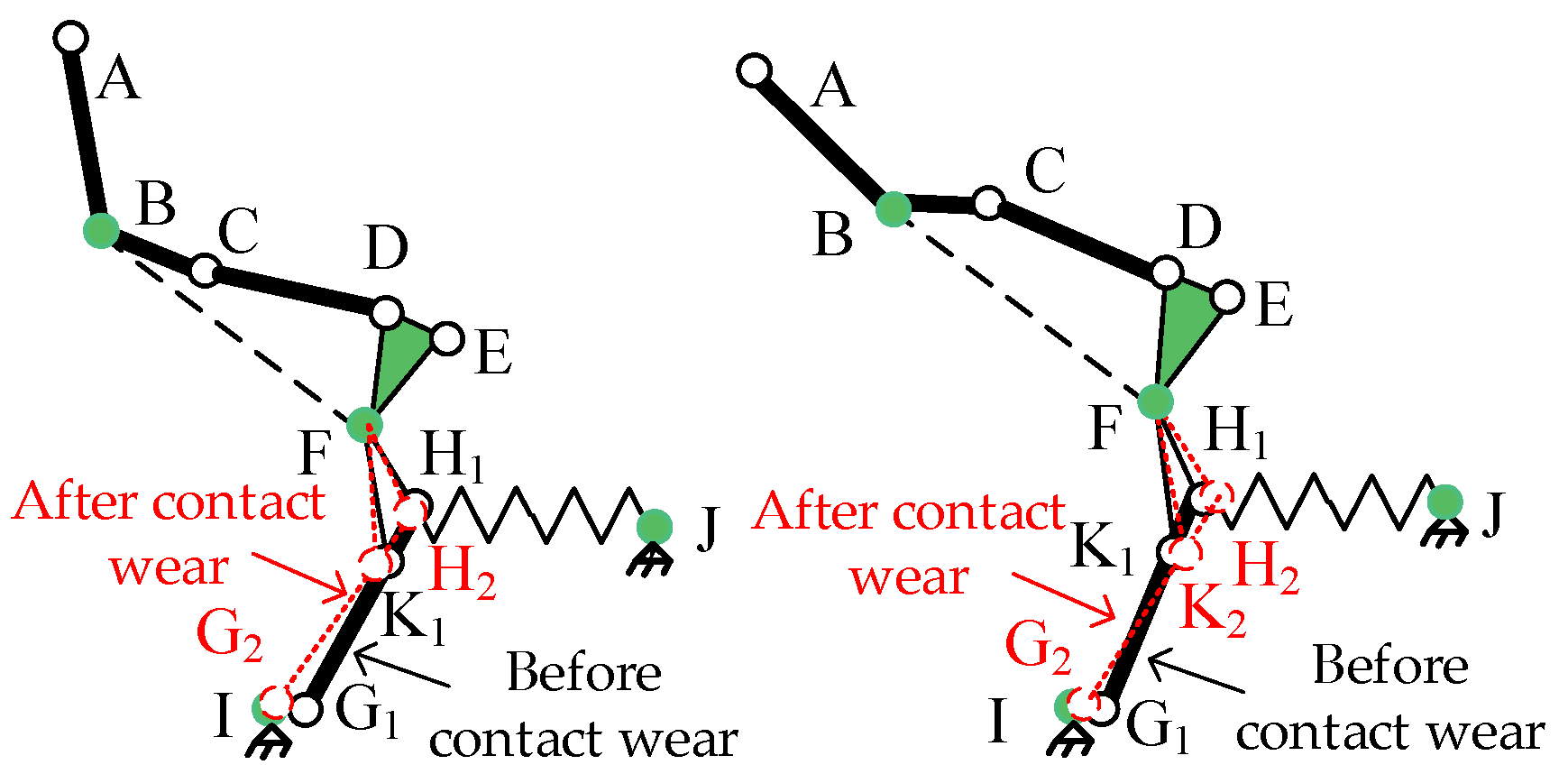
2.1. Failure Causes of MCBs

An MCB is mainly composed of a contact system, protection system, and mechanical operating system; a three-dimensional solid model is shown in Figure 1.

An MCB’s electrical life depends mainly on the degree of wear and tear of the contact system; an MCB in the connection and breaking process of the contact system will pull the arc; the high temperature generated by the arc leads to contact surface melting and wear; and at the same time, the mechanical stress between the static and dynamic contacts caused by the deformation of the contact surface aggravates the wear and tear. The arc erosion process is shown in Figure 2.

The contact mass loss of an MCB is related to the arc voltage, arc current, and arcing time, and the electrical wear model of the contact for a single break can be expressed as follows under the same current stress:

$$m_{pj}={\displaystyle {\int }_{t_q}^{t_x}f\left(i_{pj},u_{pj},t\right)}dt$$

(1)

Among them, m_pj is the loss of contact mass in the jth break of the p phase. p = 1, 2, and 3 are three phases, which are A, B, and C, respectively. Moreover, i_pj(t) is the instantaneous value of the arc current of the jth breaking of phase P, UPJ(T) is the instantaneous value of the arc voltage of the jth breaking of phase P, t_q is the time of arc starting, and t_x is the time of arc quenching.

$${\displaystyle {\int }_{t_q}^{t_x}f\left(i_{pj},u_{pj},t\right)}dt=K\cdot g_{pj}$$

(2)

where g_pj is the characteristic quantity of the ignited arc and K is the arc erosion coefficient, which is used to describe the relationship between the contact mass loss and the ignited arc parameters, and it is related to contact parameters such as the arc extinguishing system, the contact motion speed, the contact material and the structure, which can be obtained from the experimental and historical data. After determining the MCB structure and contact material, the three-phase contacts are basically the same, so it can be considered that under the same current stress, the three-phase contacts have the same arc erosion coefficient. Based on the above analysis, Equation (3) can be derived.

$$m_{pj}=K\cdot g_{pj}$$

(3)

If the arc erosion factor K is known, then Equation (3) can be utilized to calculate the product’s single-breaking contact mass loss. After the number of operations T, the cumulative contact mass loss is as follows:

$${\displaystyle \sum _{j=1}^T{m}_{pj}}={\displaystyle \sum _{j=1}^{T}K\cdot g_{pj}}=K\cdot {\displaystyle \sum _{j=1}^T{g}_{pj}}$$

(4)

With the increase in the number of MCB actions, mechanical stress, arc erosion, and other factors on the contacts to produce the cumulative damage effect are more and more serious, and frequent breaking of the circuit occurs so that the arc erosion of the contact material is too much; then, the contact pressure between the contacts falls too much resulting in static and dynamic contacts that cannot be reliably contacted. Today’s MCB product performance is very mature, its structural design is reasonable, and in the service process of MCBs its mechanical life far exceeds its electrical life, which is the contact failure for the MCB’s main failure form.

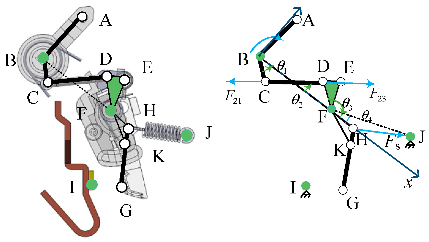
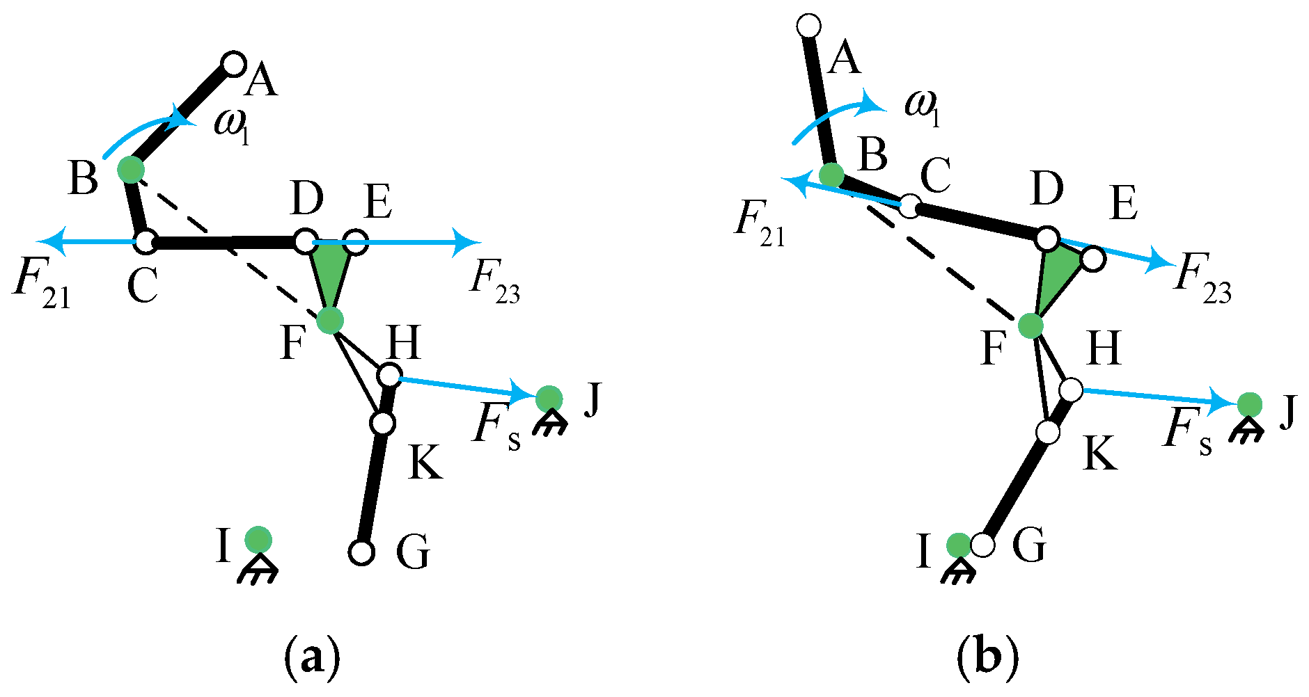
2.2. Closing Process Analysis

The operational performance of miniature circuit breakers is mainly determined by the operating mechanism and the contact system. Wear, fracture, or other issues in any mechanical component of the mechanism can lead to changes in the mechanism’s movement. The operating mechanism consists of components such as the handle BC, U-shaped connecting rod CD, trip latch DE, lock catch DF, contact lever FG, and central support DEKF. According to the motion characteristics and coordination relationships of different components during the closing and opening processes, some irregularly shaped components are equivalent to connecting rods of certain lengths. The equivalent operating mechanism model is used to analyze the mechanism’s behavior during closing and opening processes. Taking point B of the handle as the origin, the straight line connecting with the shaft pin F as the x-axis, and the straight line perpendicular to the x-axis as the y-axis, a plane rectangular coordinate system is established. Let the handle BC be rod 1, the U-shaped connecting rod CD be rod 2, and the distance DF from articulation point D to shaft pin F be rod 3. The force analysis diagram of the mechanism in the initial position and the schematic diagram of the operating mechanism and its equivalent mechanism are shown in Figure 3.

According to the relative motion relationship between the moving and stationary contacts, the closing process of the miniature circuit breaker is divided into an idle-stroke phase and an overtravel phase. The idle-stroke phase refers to the process from the rotation of the handle to just before the moving and stationary contacts make contact. Assuming the handle rotates at a constant angular velocity ω₁, during the idle-stroke phase, the handle drives the U-shaped connecting rod and the contact assembly to move in the form of a four-bar linkage; the motion process is shown in Equation (5) and Figure 4.

$$\left\{\begin{array}{l}{\theta }_2=\arcsin ({\displaystyle \frac{l_{\mathrm{DF}}\sin {\theta }_3-l_{\mathrm{BC}}\sin {\theta }_1}{l_{\mathrm{CD}}}})\hfill \\ {\theta }_3=\pi -\arcsin ({\displaystyle \frac{l_{\mathrm{BC}}\sin {\theta }_1}{l_{\mathrm{CF}}}})-\arccos ({\displaystyle \frac{l_{\mathrm{CF}}^2+l_{\mathrm{DF}}^2-l_{\mathrm{CD}}^2}{2\cdot l_{\mathrm{CF}}\cdot l_{\mathrm{DF}}}})\hfill \\ {\omega }_2={\displaystyle \frac{-{\omega }_1{l}_{\mathrm{BC}}\sin ({\theta }_1-{\theta }_3)}{l_{\mathrm{CD}}\sin ({\theta }_2-{\theta }_3)}}\hfill \\ {\omega }_3={\displaystyle \frac{{\omega }_1{l}_{\mathrm{BC}}\sin ({\theta }_1-{\theta }_2)}{l_{\mathrm{DF}}\sin ({\theta }_3-{\theta }_2)}}\hfill \\ {\ddot{\theta }}_3={\displaystyle \frac{{\omega }_1^2{l}_{\mathrm{BC}}\cos ({\theta }_1-{\theta }_2)+{\omega }_2^2{l}_{\mathrm{CD}}-{\omega }_3^2{l}_{\mathrm{DF}}\cos ({\theta }_3-{\theta }_2)}{l_{\mathrm{DF}}\sin ({\theta }_3-{\theta }_2)}}\hfill \end{array}\right.$$

(5)

In the formula, θ₂ and θ₃ are the rotation angles of rods 2 and 3; ω₂ and ω₃ are the rotational angular velocities of rod 2 and rod 3, respectively; and ${\ddot{\theta }}_3$ is the rotational angular acceleration of rod 3.

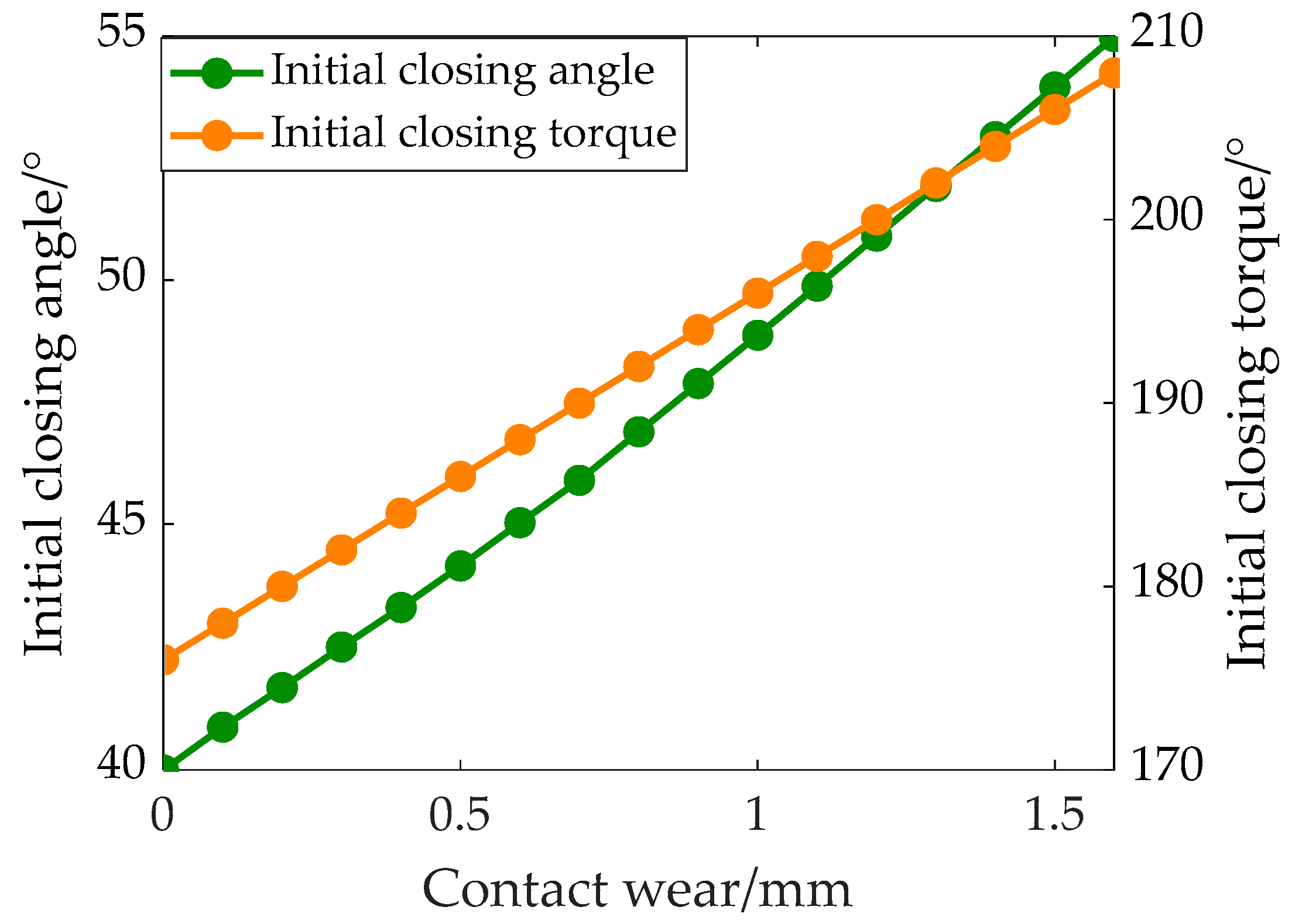
2.3. Dynamic Simulation Analysis

This section uses the multi-body dynamic simulation software ADAMS 2018 to establish a virtual prototype model of the miniature circuit breaker operating mechanism, simulating the movement patterns of each component of the operating mechanism during the closing process. Apply contact forces and other constraints between the components of the MCB. Set the handle drive mode to constant-speed drive. Use the parameters obtained from the actual measurements to set the stiffness coefficients of the torsion spring and contact spring. Define the rotation angle of the handle. Finally, obtain the virtual prototype model of the MCB, where the counterclockwise arrow at the handle indicates the drive, and the counterclockwise arrows at other hinge points indicate the rotating joints. The lock shape indicates a fixed joint. The dynamic simulation model is shown in Figure 5.

The relationship between the operating torque of the handle and the angle of the rotation of the handle during the closing process was obtained through simulation, as shown in Figure 6.

The initial closing angle is the angle of rotation of the handle from the start of rotation to the point where the contacts close. Based on the curve changes during the closing process, it can be seen that the closing angle can characterize the operating status of the circuit breaker. Therefore, the closing angle is selected as the characteristic parameter.

The initial closing angle is the angle of rotation of the handle from the start of rotation to the point where the contacts close, and the initial closing torque is the torque of the handle from the start of rotation to the point where the contacts close. Based on the curve changes during the closing process, it can be seen that the initial closing angle and initial closing torque can characterize the operational status of the circuit breaker.

With the increase in the number of MCB operations, the amount of contact wear gradually increases. Before and after the contact wear dynamic and static contacts contact when the mechanical mechanism position changes, as shown in Figure 7, H₁, K₁, and G₁ indicate the contact intact case of the location of the components, and H₂, K₂, and G₂ indicate the contact wear case of the location of the components.

The trend of the initial closing angle change with the contact wear is simulated through dynamic simulation, as shown in Figure 8.

As can be seen from Figure 8, both the initial closing angle and the initial closing torque show a linear trend with the amount of contact wear. In order to verify the linear variation, the linear correlation analysis between the characteristic quantity and the change in contact wear was carried out; the correlation coefficients between the initial closing angle, the initial closing torque, and the contact wear were 0.99915 and 0.99875, respectively; and the absolute value was greater than 0.9, so it can be considered that the initial closing angle and initial closing torque of the MCB increased linearly with the contact wear. After the sensitivity analysis of the changes in the two eigenquantities, the sensitivities of the rigidity angle and rigidity moment were 27.33% and 14.56%, respectively, as shown in Figure 9, so the rigidity angle is selected as the eigenquantity for the remaining life prediction.

3. Electrical Life Prediction Method for MCBs

3.1. Electrical Performance Degradation Model

The contact degradation process of MCBs is a contact thickness decreasing and non-monotonic degradation process, which meets the conditions for the application of the Wiener process, so a one-dimensional linear Wiener process is chosen to describe the electrical performance degradation process of MCBs.

The contact mass loss m for a single interruption of an MCB does not follow a normal distribution. However, if the single contact mass loss m is divided into segments and accumulated, the accumulated contact mass loss for each segment follows a normal distribution. In the test, one segment is accumulated for every k times of opening, and the accumulated contact mass loss of each segment is recorded as ΔM; its expression is as follows:

$$\Delta M=\sum _{j=1}^k{m}_j$$

(6)

where m_j denotes the contact mass loss incurred at the jth operation of the circuit breaker, and j denotes the jth opening of the MCB.

As the arc starting phase angle of the arc is generated randomly during each opening, after the arc erodes the contact many times, it can be regarded that the arc uniformly wears out the contact, the thickness of the contact is uniformly reduced, the cumulative contact mass loss can be transformed into the cumulative contact thickness loss by (7), and both of them obey the normal distribution.

$$\Delta H={\displaystyle \frac{\Delta M}{\rho S}}$$

(7)

where ρ denotes the contact material density, S denotes the area of the contact loss region after breaking, and ΔH denotes the thickness of the accumulated contact loss.

According to the central limit theorem, when k is large, there is the following relation.

$${\displaystyle \frac{\Delta H-k{\mu }_H}{\sqrt{k}{\sigma }_H}}~N(0,1)$$

(8)

In the formula, µ_H is the average contact thickness loss, and σ_H is the standard deviation of the contact thickness loss.

The initial closing angle can be used as a degradation characterization quantity for the remaining electrical life prediction of the MCB, where the cumulative degradation of the initial closing angle is denoted as Y(t), the degradation increment is ΔY~N(µ_Y, σ_Y²), and the MCB conforms to the nature of the one-dimensional Wiener process so that µ₁ = kµ_Y, σ₁² = kσ_Y²; the electrical performance degradation is modeled as follows:

$$Y\left(t\right)={\mu }_{1}t+{\sigma }_1{B}_1\left(t\right)$$

(9)

where Y(t) is the cumulative degradation of the initial closing angle and Y(t)~N(µ₁t, σ₁²t), µ₁ is the rate of degradation of the electrical performance of the MCB, and σ₁ is a diffusion parameter, which indicates the randomness of the arc erosion of contacts and the influence of contingent factors, such as the existence of experimental errors, on the performance of an MCB.

The above model parameters are estimated by the great likelihood estimation method, and the parameter estimation formula is shown in (10).

$${\displaystyle \left\{\begin{array}{c}{\widehat{\mu }}_1={\displaystyle \frac{1}{\mathrm{kN}}}{\displaystyle \sum _{i=1}^N}\Delta Y_i\\ {{\widehat{\sigma }}_1}^2={\displaystyle \frac{1}{\mathrm{kN}}}{\displaystyle \sum _{i=1}^N}{(\Delta Y_i-{\widehat{\mu }}_{1}k)}^2\\ \widehat{L}={\displaystyle \sum _{i=1}^N}\Delta Y_i\end{array}\right.}$$

(10)

where k is the cumulative number of MCB closures and openings per segment, N is the number of measurements of the initial closing angle degradation, and ΔY_i is the incremental initial closing angle degradation at the ith measurement.

3.2. Residual Electric Life Prediction Model

When the average degradation rate of the MCB is a constant value, the electrical life of the MCB can be defined as the number of operations when the cumulative degradation reaches the failure threshold for the first time, and its remaining life prediction principle is shown in Figure 10.

When the cumulative degradation Y(t) of a phase of the MCB at the initial closing angle reaches the failure threshold L for the first time, it can be considered that the MCB undergoes an electrical degradation failure. Therefore, the MCB electrical life T can be defined as follows:

$$T=\inf \{t\left|Y\right(t)\ge L,Y\left(0\right)\le L\}$$

(11)

Since the time distribution of the Wiener process up to a certain point obeys the inverse Gaussian distribution, when the cumulative degradation of the initial closing angle Y(t) has not yet reached the failure threshold L, set L′ = L − L₀, where L₀ is the current cumulative degradation, and the probability density function of the electric life at the current degradation moment is as follows.

$$\mathrm{f}(t)={\displaystyle \frac{L^{\prime }}{\sqrt{2\pi t^3}{\sigma }_1}}\exp \left[-{\displaystyle \frac{{(L^{\prime }-{\mu }_{1}t)}^2}{2{{\sigma }_1}^{2}t}}\right]$$

(12)

The electrical life distribution function and reliability function of the MCB operating to the current moment are, respectively, as follows:

$$R(t)=\mathsf{\Phi }\left({\displaystyle \frac{L^{\prime }-{\mu }_{1}t}{{\sigma }_1\sqrt{t}}}\right)-\mathrm{e}\mathrm{x}\mathrm{p}\left({\displaystyle \frac{2{\mu }_1{L}^{\prime }}{{{\sigma }_1}^2}}\right)\mathsf{\Phi }\left({\displaystyle \frac{-L^{\prime }-{\mu }_{1}t}{{\sigma }_1\sqrt{t}}}\right)$$

(13)

where Φ(·) is the standard normal distribution function.

4. Simulation Results Analysis

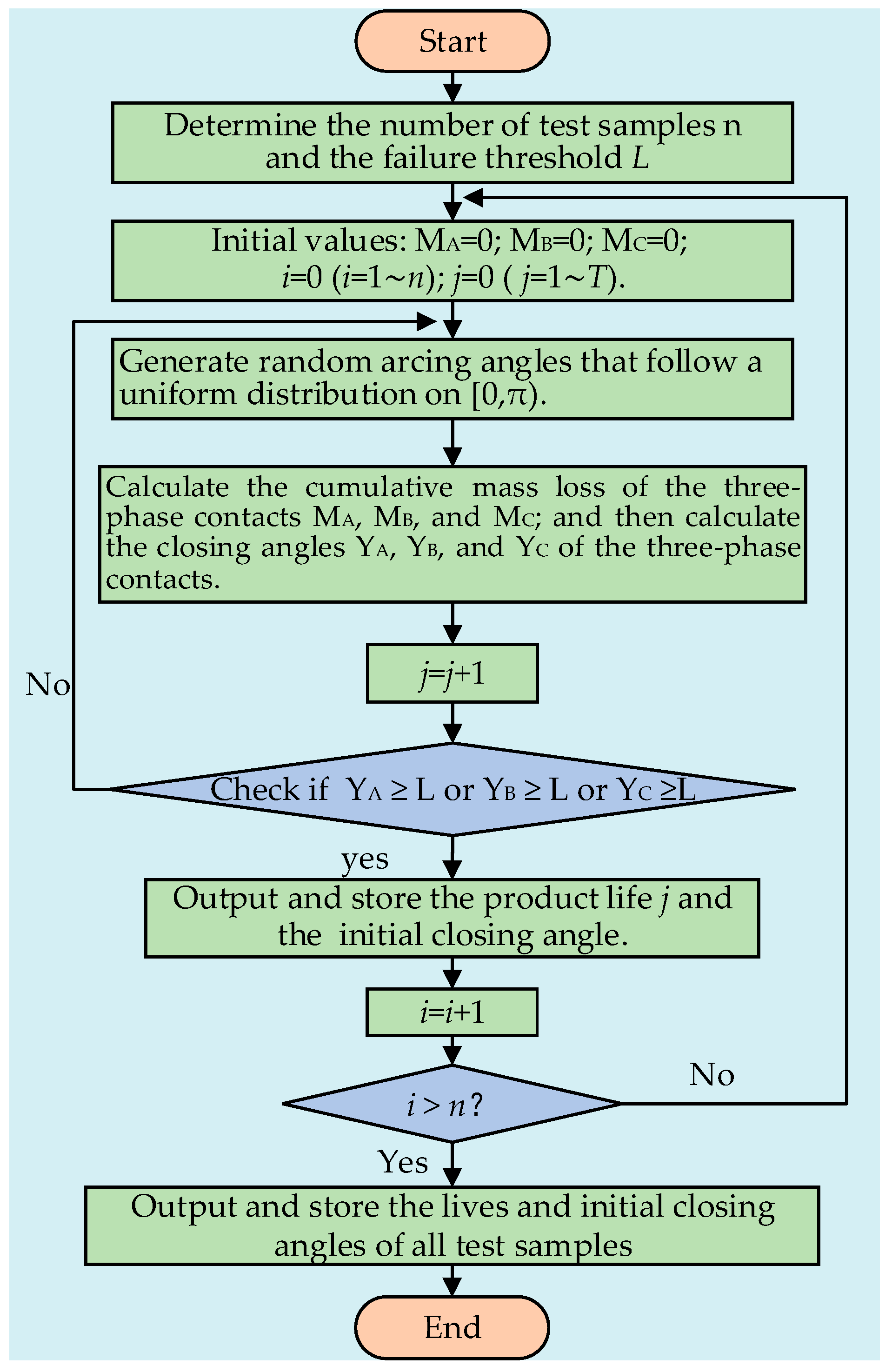
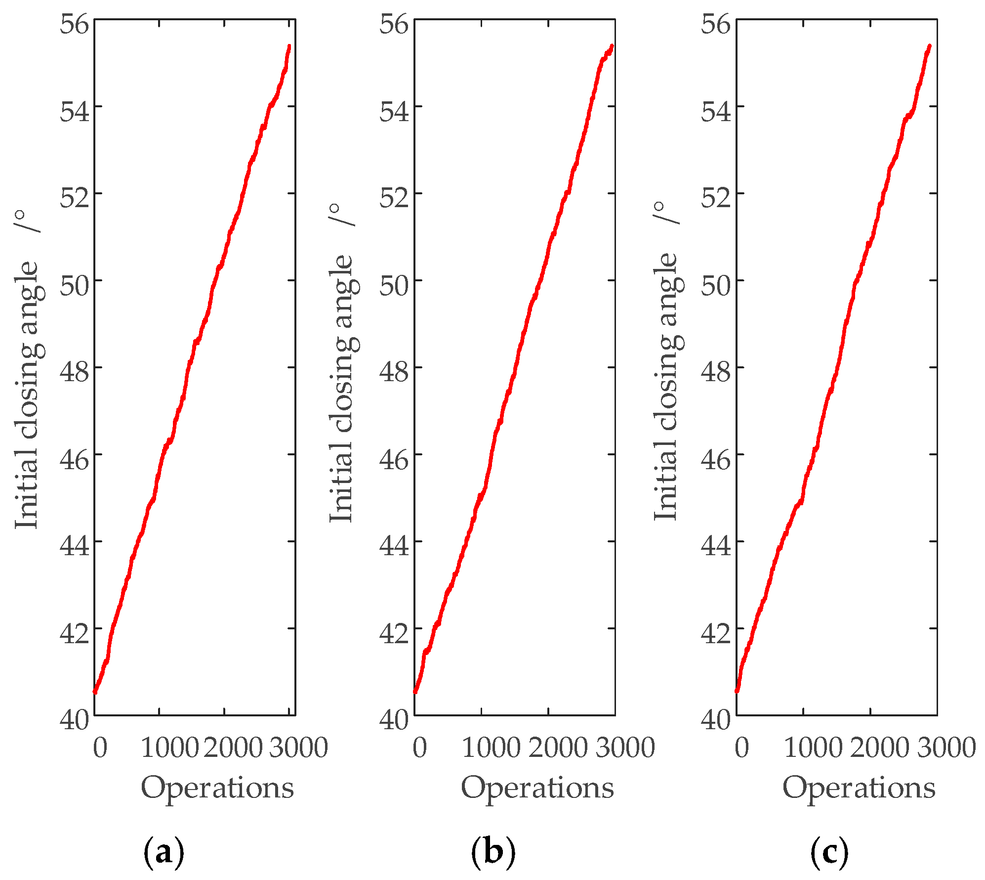
4.1. Monte Carlo Based Electrical Life Simulation

The principle of the Monte Carlo method is that the probability of an event can be estimated by the frequency of occurrence in a large number of tests. In this paper, the simulation analysis of an MCB under the uniform wear of contacts based on the Monte Carlo method is carried out to simulate the degradation process of an MCB’s electrical performance by taking the initial closing angle as the degradation eigenquantity, and the simulation steps are as follows:

(1) Input the number of MCB simulation samples and the failure threshold;

(2) Randomly generate a series of arc-starting phase angles obeying a uniform distribution in the range of [0,π);

(3) Calculate the cumulative mass loss of each phase contact and convert it to the initial closing angle of each phase contact;

(4) Calculating the initial closing angle of each phase contact with the increase in the number of operations, when the initial closing angle of any phase reaches the failure threshold, determining the end of its life, the simulation process of the sample stopsm and the number of operations at the time that is recorded as the electrical life of the sample, otherwise continuing to execute steps (1)~(3);

(5) The program repeats the execution of steps (2)~(4) for n times, and the data of the initial closing angle of n MCB simulation samples in the process of electrical degradation can be obtained.

The simulation flowchart is shown in Figure 11.

The breaking voltage is set to 380 V, load current to 63 A, and power factor to 0.65 for the simulation. In the actual service process, the MCB electrical life depends on the most serious wear of a phase, and as long as any one of the phase of the initial closing angle reaches the failure threshold, this means that the test piece cannot be reliably in service. Therefore, the initial closing of the most severely worn phase is taken as the cumulative degradation characterization of the sample. Since a larger number of simulation samples can help to reduce the chance caused by individual differences, the results can be more in line with reality. Therefore, in this section, the simulation data of 1000 samples were generated by the Monte Carlo simulation method, from which the three samples with the highest, average, and lowest electrical lifetimes, which were 3009, 2947, and 2886 times, respectively, were selected for analysis. The degradation of the initial closing angle of the three samples was accumulated every 50 times, and the variation in the initial closing angle of each of the three MCB samples with the number of operations is shown in Figure 12.

As can be seen from Figure 12, with the gradual increase in the number of MCB operations, the initial closing angles of the three samples show a significant linear increase as a whole, and the difference in the initial closing angles at the end of the electrical life is also relatively small.

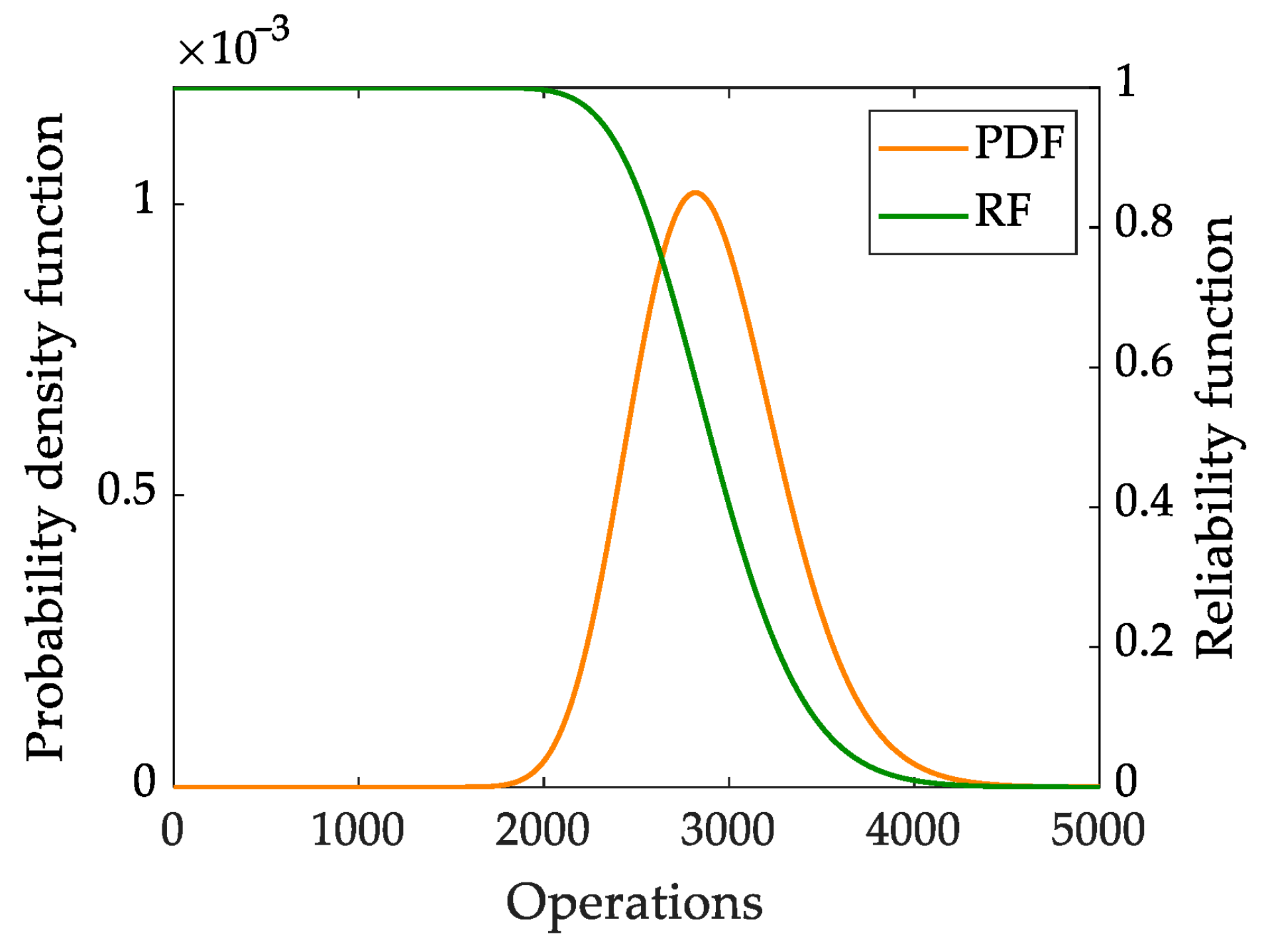
4.2. Normal Distribution Test

The K-S test was used to test the normality of the degradation increments of the initial closing angle of the three samples generated by Monte Carlo simulation. The significance level α of the K-S test was set at 0.05, and the null hypothesis was normal distribution. The results are shown in

Table 1. K-S test results of initial closing angle of simulated samples.

Case	MCB 1	MCB 2	MCB 3
Test statistic	0.0614	0.0757	0.0645
Threshold value	0.27	0.24	0.23
Obedience test	obey	Obey	obey

.

As can be seen from Table 1, in the K-S test of the degradation increment of the initial closing angle of each of the three samples, the test statistic is smaller than the critical value, the two test methods sufficiently show that the degradation increment of the initial closing angle of the various segments obeys the normal distribution, and the Wiener process can be adopted to describe the electrical performance degradation process of MCBs. The Wiener process describes the degradation process of the electrical properties of MCBs.

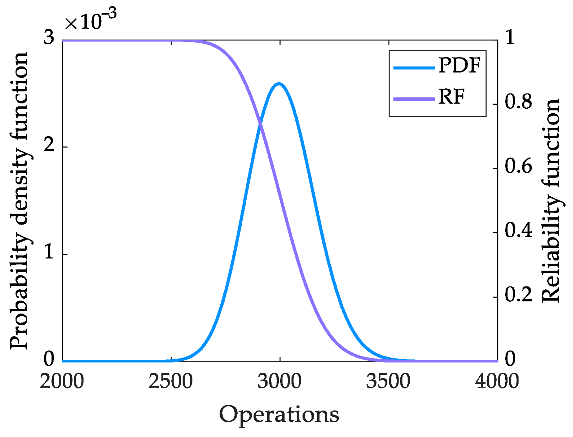
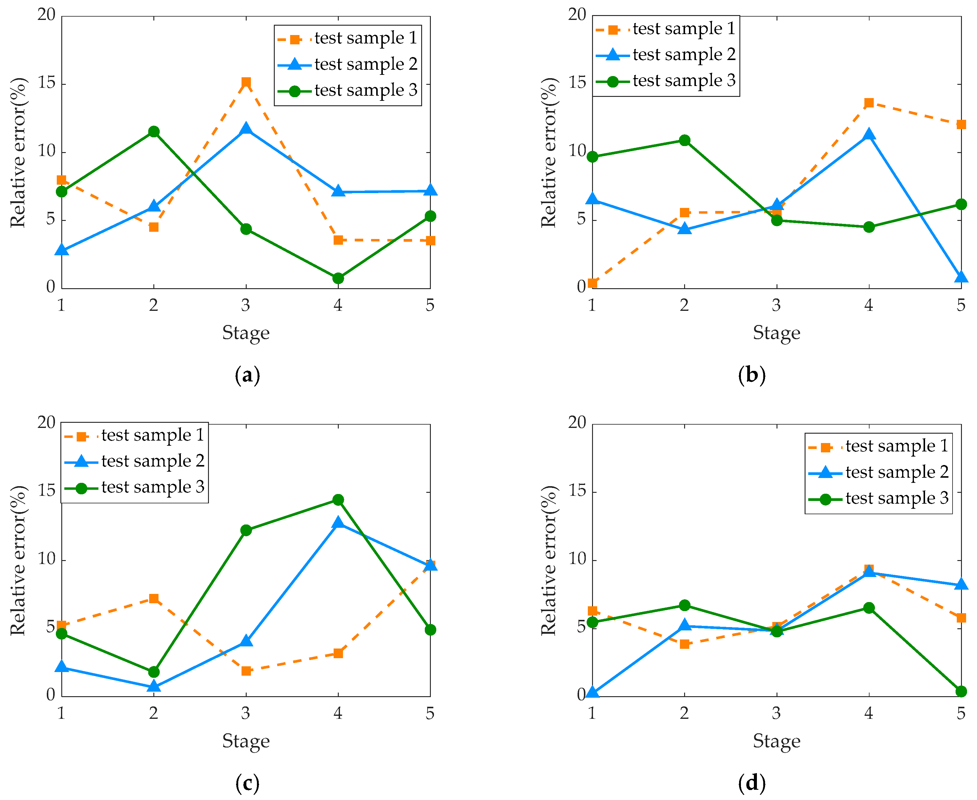
4.3. Residual Electrical Life Prediction Based on Simulation Data

Based on the initial closing angle degradation data obtained from the Monte Carlo simulation, the electrical life prediction for sample 1 was selected. The parameter estimation of the electrical life prediction model was carried out through Equation (6), and the estimated values of the model parameters for the three samples as well as their average values were obtained. The results are shown in

Table 2. Parameter estimates of the degradation model.

Parameters	µ1 Estimated Value	σ1 Estimated Value
MCB 1	0.005	0.0138
MCB 2	0.0049	0.0138
MCB 3	0.0048	0.0138
Average value	0.0049	0.0138

.

The electrical life prediction of the MCB is carried out by taking MCB 1 as an example, the estimated values of the model parameters derived in Table 2 are substituted into Equations (12) and (13) to obtain the electrical life probability density function and reliability function of test article 1, and the curves are shown in Figure 13.

$$\mathrm{f}\left(t\right)={\displaystyle \frac{14.73}{0.0138\sqrt{2\pi t^3}}}\exp \left[-{\displaystyle \frac{{\left(14.73-0.0049t\right)}^2}{0.0004t}}\right]$$

(14)

$$\mathrm{R}\left(t\right)=\mathsf{\Phi }\left({\displaystyle \frac{14.73-0.0049t}{0.0389\sqrt{t}}}\right)-\exp \left(763.4985\right)\mathsf{\Phi }\left({\displaystyle \frac{-14.73-0.0049t}{0.0138\sqrt{t}}}\right)$$

(15)

As can be seen in Figure 13, after about 2500 closing and closing operations, the reliability of sample 1 starts to decrease rapidly. The predicted electrical life of sample 1 is 2989 times, and the simulated electrical life is 3009 times, with a relative error of 0.7%, and the predicted and simulated electrical lives are very similar. In order to further verify the accuracy of the electrical degradation process, the estimated values of sample 2 and sample 3 and the mean drift parameter and diffusion parameter in Table 2 were substituted into Equations (14) and (15), and the expected values of the respective probability density functions were 2988, 2975, and 2990 times, which were also close to the simulated electrical life, with the relative errors of 0.7%, 1.13%, and 0.6%, respectively, which were accurate in the prediction results.

On this basis, the remaining electric life prediction of the MCB in different service stages was carried out, and still taking sample 1 as an example, after its electric life was divided into five stages, the current cumulative degradation amount L₀ and the estimated values of the model parameters in different service stages were substituted into Equation (12) to calculate the predicted value of the remaining electric life of the sample 1 in different service stages and compare it with the corresponding stage of the remaining life simulation value. They are shown in

Table 3. Prediction of the remaining electrical life of sample 1 at different stages.

Stage	Actual Residual Electric Life	Prediction of Remaining Electrical Life	Relative Error
1–500	2509	2465	3.80%
501–1000	2009	1965	1.29%
1001–1500	1509	1429	3.68%
1501–2000	1009	957	1.76%
2001–2500	509	497	2.36%

. The residual electric life prediction errors of sample 1 in different stages are less than 4%, and the prediction results are accurate, which shows that the proposed residual electric life prediction method can realize the residual electric life prediction of individual MCBs in different stages of service more accurately.

The residual electrical life was predicted for sample 2 and sample 3 by the parameter estimates of sample 1, respectively, and the relative errors between the predicted and actual values were calculated, as shown in Figure 14a. Using this analytical method, the mean values of the parameter estimates of sample 2~3 and the samples were used to predict the remaining electrical life of sample 1~3 at different service stages, respectively.

As can be seen from Figure 14, through the model parameter values of sample 1~3 and the average values of the model parameters for the three samples to predict the remaining electrical life at different service stages, whether based on their own data or the data of other products in the same batch, the maximum prediction error at each stage is not more than 10%, which is within the acceptable range. Therefore, it is concluded from the above analysis that in the service process of MCBs, the trend of the change in the initial closing angle with the number of operations is a monotonous linear increase, and the electrical performance degradation model of MCBs can be established by using the univariate linear Wiener process and can accurately complete the prediction of residual electrical life for samples.

5. Experimental Result Analysis

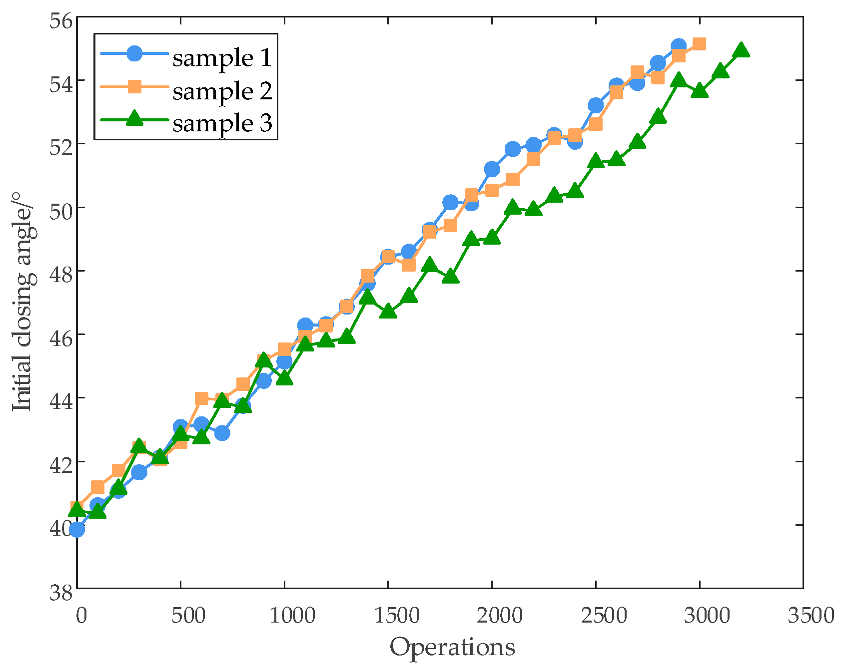
5.1. Experimental Data Analysis

This section carries out the electrical life experiments of three MCB samples with the experimental current of 63 A, and the breaking mode in the experiments is randomized. The breaking method in the experiment is random. The experimental conditions are shown in

Table 4. Parameters for life experiment.

Experimental Parameters	Numerical Value
Rated current Ie/A	63
Rated voltage Ue/V	380
Operating frequency/(times/h)	120
Coil voltage/V	380
Test current I/A	63
Test voltage U/V	380
Power supply frequency/Hz	50
Power factor	0.65
Movable contact material	AgNi(10)
Movable contact size/(mm3)	3.8 × 2 × 1.1(R)
Static contact material	AgCdO(15)
Static contact size/(mm3)	4 × 4 × 1

.

Figure 15a shows the MCB electrical life test apparatus, which mainly applies electrical stress to the MCB test sample and then performs a certain number of closing and opening operations until the MCB test sample reaches the end of its life. Figure 15b shows the MCB characteristic signal measurement and extraction apparatus, which fixes the MCB in place and then rotates the motor at a fixed speed to drive the MCB handle to rotate at a constant speed and measure the characteristic signal of the initial closing angle.

The initial closing angle of the MCB was collected after every 100 openings of the contacts, and the performance degradation data of the MCB at the rated current was analyzed. When the MCB fails to turn on after closing or fails to break when breaking, the sample is considered to have failed and the electrical life experiment of the sample is terminated. After the completion of the experiment, the electrical life of the three samples was 2897, 2989, and 3200 times, respectively.

As can be seen from Figure 16, with the increase in the number of MCB closing and breaking times, the degree of contact erosion and wear is more serious, and the contact opening distance gradually increases, which is manifested in the closing process of the overall trend of the angle just closing. This is due to the MCB opening process of the breaking arc phase angle that has a randomness of generation of the arc, and the phenomenon of the arc combustion process is accompanied by evaporation and splashing and other phenomena that make the contact material occur at different degrees of loss, as well as the uneven distribution of contact material loss and other factors that lead to the uneven ablation of the contact surface and the formation of pits and protrusions during the opening process; the high and low surface morphology makes the initial closing angle in the process with the rise of small fluctuations, but this does not affect the overall upward trend of the initial closing angle.

This batch of products uses the IT9 manufacturing tolerance standard, which ensures high production consistency. The initial values and change trends of the initial closing angles of the three samples are basically consistent, further verifying the production consistency of the products. For products with insufficient consistency, the failure thresholds of different products at the moment of complete wear can be obtained through simulation, and their distribution patterns can be analyzed. This method can convert fixed failure thresholds into distribution-based random variables, thereby reducing the impact of product inconsistency.

5.2. Normal Distribution Test

The K-S test was used to test the normal distribution of the data from the three samples.

As seen in

Table 5. K-S test results of initial closing angle.

Case	Test Statistic	Threshold Value	Obedience Test
MCB 1	0.1245	0.24	obey
MCB 2	0.1279	0.24	obey
MCB 3	0.1165	0.24	obey

, the initial closing angle degradation increment of each segment obeys a normal distribution, and the Wiener process can be used to describe the electrical degradation process of MCBs.

5.3. Experimental Data Analysis

The model parameter estimates and their mean values for each test article were calculated from Equation (10) and the estimates are shown in

Table 6. Parameter estimates of the degradation model.

Parameters	µ1 Estimated Value	σ1 Estimated Value
MCB 1	0.0052	0.0389
MCB 2	0.0049	0.0398
MCB 3	0.0045	0.0437
Average value	0.0049	0.0408

.

The electrical life prediction of the MCB is carried out as an example of test sample 1. The probability density function and reliability function of the electrical life of test sample 1 are obtained by substituting the estimated values of the model parameters derived in Table 6 into Equations (12) and (13).

$$\mathrm{f}\left(t\right)={\displaystyle \frac{15.06}{0.0389\sqrt{2\pi t^3}}}\exp \left[-{\displaystyle \frac{{\left(15.06-0.0052t\right)}^2}{0.003t}}\right]$$

(16)

$$\mathrm{R}\left(t\right)=\mathsf{\Phi }\left({\displaystyle \frac{15.06-0.0052t}{0.0389\sqrt{t}}}\right)-\exp \left(104.2543\right)\mathsf{\Phi }\left({\displaystyle \frac{-15.06-0.0052t}{0.0389\sqrt{t}}}\right)$$

(17)

As can be seen from Figure 17, after about 1992 closing and closing operations of sample 1, its reliability began to decline rapidly, indicating that, at this time, sample 1 began to leave the normal service state, the probability of failure of the MCB began to increase, and it was necessary to consider the test article for timely maintenance or replacement. The expected value of the electric life of sample 1 is 2820 times, the actual electric life is 2897 times, the prediction error is 2.7%, and the predicted electric life is very close to the actual electric life.

The estimated values of sample 2~3 and the average values of the model parameters in Table 6 are substituted into Equations (12) and (13) to predict the electrical life of sample 1. The expected values of the probability density function for the three cases are 3028, 3208, and 2964 times, which are close to the actual electrical life of sample 1, and the prediction errors are 4.5%, 10.7%, and 2.3%, respectively, which are within the acceptable range of engineering.

On this basis, the individual residual electric life prediction of MCB samples in different service stages is carried out, sample 1 is still taken as an example, its electric life is divided into five stages, the residual electric life prediction of each service stage is calculated and compared with the actual value, and the results are shown in

Table 7. Prediction of the remaining electrical life of sample 1 at different stages.

Stage	Actual Residual Electric Life	Prediction of Remaining Electrical Life	Relative Error
1–500	2397	2206	7.97%
501–1000	1897	1811	4.53%
1001–1500	1397	1344	3.79%
1501–2000	897	865	3.57%
2001–2500	397	383	3.53%

. It can be seen that the relative error of the prediction of different stages is less than 8%, and the prediction results are more accurate.

The residual electrical life was predicted for sample 2 and 3, respectively, from the parameter estimates of sample 1, and the relative errors between the predicted and actual values were calculated, as shown in Figure 18a. Using this analytical method, the mean values of the parameter estimates of sample 2~3 and the samples were used to predict the remaining electrical life of sample 1~3 at different service stages, respectively.

As can be seen from Figure 18, through the model parameter values of sample 2~3 and the average values of the model parameters of the sample to predict the residual electrical life of the three samples at different service stages, the relative error between the predicted life and the actual life in all the above cases is within 15%, which is within the acceptable range of engineering.

In summary, the initial closing angle as a performance degradation characterization quantity can better characterize the electrical performance degradation of MCBs and also shows that the residual electric life prediction model established in this paper is accurate, and in the absence of its own performance degradation data, it can be used to carry out the reliability analysis of MCBs with the degradation data of the same batch of products.

6. Conclusions

In this paper, the dynamic characteristics of an MCB are simulated and analyzed, and a residual life prediction method using the initial closing angle to characterize the MCB is proposed and studied. The main conclusions are as follows:

(1) The reasons for the degradation of MCB performance are analyzed, the MCB kinetic simulation model is established based on the kinetic characteristic analysis, and the change characteristics of the initial closing angle and the initial closing torque with the wear amount of the contact during the closing process are analyzed; moreover, through sensitivity analysis of two characteristic quantities, the initial closing angle is selected as the characteristic quantity for predicting the remaining life.

(2) Assuming that the contact thickness of the MCB decreases uniformly after multiple breakage, the relationship between the degradation of the MCB electrical performance and the initial closing angle is analyzed, and the degradation model of the MCB electrical performance is established by using a one-dimensional linear Wiener process.

(3) The electrical performance degradation simulation based on the Monte Carlo method was carried out and the remaining electrical life was predicted from the simulation data, and the prediction errors did not exceed 10%. The MCB electrical life experiments under the 63A current were carried out, the maximum likelihood estimation and degradation model were obtained from the experimental data, and the maximum prediction error of the proposed method did not exceed 15% for the MCBs of the same batch in different operation stages.

References

1. Cheng, S.; Liu, J.; Wu, X.; Yu, T.; Xiang, C.; Yuan, D. Residual life prediction of metallized film capacitors based on feature extraction and error compensation. Chin. J. Electr. Eng. 2022, 42, 2672–2681. [Google Scholar]
2. You, Y.; Wang, J.; Shu, L.; Ni, K.; Zhou, X. An electrical life prediction method for AC contactors based on audio features. J. Electrotechnol. 2021, 36, 1986–1998. [Google Scholar]
3. Sun, S.; Wang, Z.; Wang, J.; Yang, F.; Ji, W. Remaining useful life prediction for circuit breaker based on SM-CFE and SA-BiLSTM. IEEE Trans. Instrum. Meas. 2023, 72, 1–14. [Google Scholar]
4. Su, X.; Wang, L.; Zhang, Z.; Wang, D. Residual Life Prediction of Low-Voltage Circuit Breaker Thermal Trip Based on the Wiener Process. Energies 2024, 17, 1189. [Google Scholar] [CrossRef]
5. Kong, W.; Shi, J.; Du, G.; Yuan, C.; Zhang, X. Research on Life Prediction Method of Earth Leakage Circuit Breaker Based on Statistical Test. J. Electr. Eng. 2024, 19, 382–390. [Google Scholar]
6. Liu, G.; Miao, J.; Zhao, X.; Wang, Z.; Li, X. Life prediction of residual current circuit breaker with overcurrent protection based on BP neural network optimized by genetic algorithm. J. Electr. Eng. Technol. 2022, 17, 2003–2014. [Google Scholar]
7. Razi-Kazemi, A.A.; Niayesh, K.; Nilchi, R. A probabilistic model-aided failure prediction approach for spring-type operating mechanism of high-voltage circuit breakers. IEEE Trans. Power Deliv. 2018, 34, 1280–1290. [Google Scholar]
8. Li, K.; Ma, D.; Zhao, C.; Hu, B.; Wang, H. Prediction of the remaining electrical life of AC contactors based on Bayesian inference. J. Instrum. Meas. 2024, 45, 34–45. [Google Scholar]
9. Chen, K.; Wang, F.; Li, H.; Gao, H.; Xia, Y.; Liu, Y. Remaining Life Prediction of High-Voltage Circuit Breakers Based on Optimized Particle Swarm-Bidirectional Long Short-Term Memory Neural Network. In Proceedings of the 2024 7th International Conference on Electric Power Equipment-Switching Technology (ICEPE-ST), Xiamen, China, 10–13 November 2024; IEEE: Piscataway, NJ, USA, 2024; pp. 697–701. [Google Scholar]
10. Huang, K.; Zhao, S. Evaluation of residual service life of high voltage circuit breaker. In Proceedings of the 2012 China International Conference on Electricity Distribution, Shanghai, China, 10–14 September 2012; IEEE: Piscataway, NJ, USA, 2012; pp. 1–4. [Google Scholar]
11. Lu, C.; Wang, C.; Xie, J. Online estimation of residual electrical lifetime for PV low voltage circuit breaker based grey algorithm. In Proceedings of the 2023 IEEE 3rd International Conference on Power, Electronics and Computer Applications (ICPECA), Shenyang, China, 29–31 January 2023; IEEE: Piscataway, NJ, USA, 2023; pp. 1216–1220. [Google Scholar]
12. Yang, J.; Chi, C. The Prediction of Residual Electrical Life in Alternating Current Circuit Breakers Based on Savitzky-Golay-Long Short-Term. Sensors 2023, 23, 6860. [Google Scholar]
13. Wu, T.; Yao, Y.; Li, Z.; Chen, B.; Wu, Y.; Sun, W. Remaining useful life prediction of circuit breaker operating mechanisms based on wavelet-enhanced dual-tree residual networks. J. Power Electron. 2024, 24, 78–91. [Google Scholar]
14. Ma, H.; Zhou, S.; Gao, C.; Zhou, F.; Yang, Y.; Yang, H. Research on the Reliability Test and Life Assessment Methods of Relays Used in Circuit Breaker Operating Mechanism. Energies 2023, 16, 4843. [Google Scholar] [CrossRef]
15. Cao, P.; Li, J.; Han, Y.; Shi, S.; Wang, Q.; Peng, Z.; Zhou, G. Mechanical remaining Life Prediction of Circuit Breaker based on long-term and short-term memory Neural Network. In Proceedings of the 2023 IEEE 6th International Electrical and Energy Conference (CIEEC), Hefei, China, 12–14 May 2023; IEEE: Piscataway, NJ, USA, 2023; pp. 2734–2738. [Google Scholar]
16. Zhao, X.; Wu, G.; Yang, D.; Xu, G.; Xing, Y.; Yao, C.; Abu-Siada, A. Enhanced detection of power transformer winding faults through 3D FRA signatures and image processing techniques. Electr. Power Syst. Res. 2025, 242, 111433. [Google Scholar] [CrossRef]
17. Su, X.; Zhang, Z.; Wei, J. Remaining Useful Life Prediction of Electromagnetic Release Based on Whale Optimization Algorithm—Particle Filtering. Energies 2024, 17, 670. [Google Scholar] [CrossRef]
18. Aizpurua, J.I.; Catterson, V.M.; Abdulhadi, I.F.; del Carmen Segovia García, M. A model-based hybrid approach for circuit breaker prognostics encompassing dynamic reliability and uncertainty. IEEE Trans. Syst. Man Cybern. Syst. 2017, 48, 1637–1648. [Google Scholar]
19. Liu, G.; Wang, L.; Yang, Y.; Liu, D.; Miao, J. Life prediction of residual current circuit breaker with overcurrent protection based on Tweedie exponential dispersion process with random effects. Electr. Eng. 2024, 107, 7027–7039. [Google Scholar]
20. Zhao, S.; Yan, X.; Wang, B.; Wang, E.; Ma, L. Research on reliability evaluation method of DC circuit breaker based on Markov model. Electr. Power Syst. Res. 2019, 173, 1–5. [Google Scholar]
21. Li, K.; Zhao, C.; Niu, F.; Zheng, S.; Duan, Y.; Huang, S.; Wu, Y. Electrical performance degradation model and residual electrical life prediction for AC contactor. IEEE Trans. Compon. Packag. Manuf. Technol. 2020, 10, 400–417. [Google Scholar]
22. Khoddam, M.; Sadeh, J.; Pourmohamadiyan, P. Performance evaluation of circuit breaker electrical contact based on dynamic resistance signature and using health index. IEEE Trans. Compon. Packag. Manuf. Technol. 2016, 6, 1505–1512. [Google Scholar]
Figure 1. Schematic diagram of MCB structure.
Energies 18 03639 g001
Figure 2. Wear process during contact closure and opening.
Energies 18 03639 g002
Figure 3. Operating mechanism and its schematic diagram of miniature circuit breaker.
Energies 18 03639 g003
Figure 4. Schematic diagram of the operating mechanism motion during the idle-stroke phase of a miniature circuit breaker. (a) Initial position; (b) contact touching position.
Energies 18 03639 g004
Figure 5. Virtual mockup model of miniature circuit breaker dynamics.
Energies 18 03639 g005
Figure 6. Simulation waveform of operating torque of handle during closing process.
Energies 18 03639 g006
Figure 7. Schematic diagram of the position change in the mechanism before and after contact wear.
Energies 18 03639 g007
Figure 8. Relationship between wear of contact and characteristic quantity.
Energies 18 03639 g008
Figure 9. Sensitivity analysis of eigenquants.
Energies 18 03639 g009
Figure 10. Schematic diagram of remaining electrical life prediction.
Energies 18 03639 g010
Figure 11. Monte Carlo simulation steps of MCBs.
Energies 18 03639 g011
Figure 12. Change in the initial closing angle of the simulated samples. (a) MCB 1; (b) MCB 2; (c) MCB 3.
Energies 18 03639 g012
Figure 13. Reliability function and probability density function of simulated sample 1.
Energies 18 03639 g013
Figure 14. Prediction results of the remaining electrical life of the 3 simulated samples. (a) Based on data from simulated sample 1; (b) based on data from simulated sample 2; (c) based on data from simulated sample 3; (d) based on the average of 3 simulated samples.
Energies 18 03639 g014
Figure 15. Electrical life test setup. (a) Electrical life test equipment; (b) measuring equipment.
Energies 18 03639 g015
Figure 16. Change in the initial closing angle of the 3 samples at the rated current.
Energies 18 03639 g016
Figure 17. Reliability function and probability density function of experimental sample 1.
Energies 18 03639 g017
Figure 18. Prediction results of the remaining electrical life of the 3 experimental samples. (a) Based on data from experimental sample 1; (b) based on data from experimental sample 2; (c) based on data from experimental sample 3; (d) based on the average of 3 experimental samples.
Energies 18 03639 g018